Abstract
It has been suggested in the literature that by reducing the incoming voltage at a distribution feeder head or at the supply side of buildings, significant electricity savings can be achieved. This technique is called Conservation Voltage Reduction (CVR). Data-based analysis with and without CVR is primarily used to support such assertions, which does not explain the physics behind reduction in energy consumption with CVR. This paper presents a new approach for evaluating the impact of CVR on cooling equipment. In this approach, a thermal-electric model of the cooling process is developed in MATLAB’s SIMSCAPE toolbox that can be used to explain the physics behind energy reduction with CVR. This model includes an accurate model of a compressor coupled to an induction motor whose supply voltage can be varied to simulate CVR. Simulations performed using this model show that the Coefficient of Performance (COP) of cooling equipment improves with a reduction in supply voltage. However, the energy lost in the motor windings may nullify the impact of the improvement in the COP and render the CVR programs ineffective if the range of speed change is small over the allowable voltage change. The simulation results show an increase in energy consumption of 4% at 90% rated voltage compared to the energy consumed at the rated voltage. However, if variable frequency drives-based cooling equipment is appropriately controlled, it is possible to reduce their net energy consumption using CVR. Simulations performed keeping the ratio of the supply voltage and the frequency constant showed a reduction in energy consumption of 2.5% at 90% rated voltage compared to the energy consumed at the rated voltage. Thermal-electric modeling of building cooling equipment is, therefore, vital to accurately evaluating the benefits of CVR as smart, power electronics-based end-use equipment is globally adopted.
1. Introduction
Energy conservation is one of the key strategies for combating climate change. There are several examples across the world where a significant reduction in energy consumption and greenhouse gas emissions has been achieved through energy conservation programs. In the United States (US), various energy efficiency programs have ensured around 23% less annual energy consumption [1]. In India, the number of LED bulbs being used between 2014 and 2018 increased from 5 million to 670 million resulting in energy savings of 30 terawatt hours () [2]. Energy conservation will continue to play a critical role in the future as the entire world strives to reduce greenhouse gas emissions and contain the average temperature rise from the beginning of the industrial age to less than 1.5 degrees by 2050 [3].
There are many tools and techniques to reduce power consumption. One such tool is Conversation Voltage Reduction (CVR), which has been used in the past and can be used in the future to reduce electricity consumption. As the name suggests, CVR involves reducing voltage at the feeder head of an electricity distribution network, or at the source-side of a commercial or industrial building to reduce electricity consumed by loads. Several researchers and utilities have used CVR to reduce power consumption [4,5,6,7,8].
In [9], an experiment was performed to evaluate the effects of CVR on electric home appliances. It was observed that in the case of constant resistive load, the power consumption decreased with a reduction in the supply voltage. However, in the case of constant power loads, a reduction in the supply voltage at the same power level resulted in an increased current demand leading to higher line losses. This highlights the importance of knowing the load model(s) to evaluate the effectiveness of CVR. In [10], the authors performed a comprehensive review of CVR implementation and discussed different methods to quantify its effects and arrived at the conclusion that while the simulation method can provide high precision, its accuracy depends on the load models used. However, no details were provided in this paper that would allow thermal-electric modeling of the cooling processes. In [11], an attempt was made to model cooling as a thermal-electric process for large-scale distribution simulations by expressing heat flow through a cooling unit as a function of voltage, ambient temperature, and Coefficient of Performance (COP). However, the explanation for the modeled thermal-electric coupling was not provided (e.g., how change in voltage affects mass flow rate and heat transfer). In [12], the authors carried out an experiment in which they operated equipment that worked at two voltage levels, 208 V and 480 V, and calculated energy savings and peak load savings for a 5% reduction in voltage. CVR and its implementation on the power systems of Washington EMC and the facilities of the Georgia Transmission Corporation were discussed in [13]. To measure, test, and verify the CVR system effects, and to obtain a reduction in peak demand and energy, an electric utility implemented a conservation voltage reduction system on its various distribution substations in [14].
The literature review on CVR reveals that while the benefits of using CVR on power consumption have been reported, modeling-based explanations for energy reduction by reducing voltage in cooling equipment are missing. Moreover, the results in the literature are for conventional loads that are increasingly being replaced with power electronics-based equipment such as inverter-air conditioners and refrigerators. The response of such electrical cooling equipment to CVR will be significantly different from those observed in conventional cooling equipment. To address these gaps, accurate thermal-electric models of cooling processes are required, where both conventional and power electronics-based cooling equipment can be simulated under CVR. This paper attempts to address these gaps by developing a MATLAB/SIMSCAPE-based thermal-electric model of the cooling process using a refrigerator as an example. Several experiments were performed using this model to identify the key reasons for reduction in energy consumption under CVR and the impact of CVR on conventional and power electronics-based cooling equipment performance. In the process, a foundation has been laid for a thorough CVR impact analysis in the future as appliance characteristics change.
The remainder of the paper is organized as follows. Section 2 presents the research methodology, where thermal-electric modeling of the refrigeration/air-conditioning process, compressor modeling, and three-phase induction motor modeling are discussed. Simulation results and major observations regarding the impact of CVR on cooling equipment performance are presented in Section 3. Experimental validation of simulation results is presented in Section 4 while Section 5 concludes this paper and identifies topics for future research.
2. Methodology
2.1. Thermal Model of Cooling Process
A thermal model of cooling process is shown in Figure 1, which is obtained from an in-built example in MATLAB-SIMSCAPE titled “ssc_refrigeration” [15]. This model explains the two-phase fluid refrigeration in which the refrigerant undergoes a phase change from liquid to vapor and back to liquid. The refrigerant fluid is compressed by the compressor, which increases its pressure and temperature. The high-pressure, high-temperature fluid then flows into the condenser, where it releases heat to the surrounding environment and condenses into a liquid. The liquid refrigerant then passes through the expansion valve, which reduces its pressure and causes it to undergo a phase change from liquid to gas (vapor). This cold, low-pressure vapor then flows into the evaporator, where it absorbs heat from the desired area and undergoes a phase change to become liquid again [16,17]. The mass and energy balance equations for the colling process are given below.
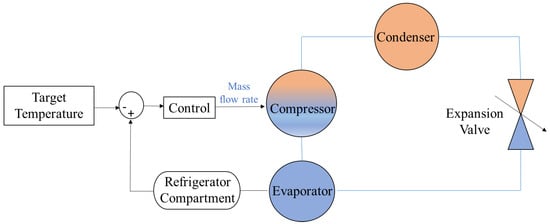
Figure 1.
Block diagram of MATLAB simulation representation of two-phase fluid refrigeration system [15].
For the compressor
For the condenser
For the expansion valve
For the evaporator
where
, are the mass flow rates of refrigerant entering and leaving the compressor, respectively.
, are the mass flow rates of refrigerant entering and leaving the condenser, respectively.
, are the mass flow rates of refrigerant entering and leaving the expansion valve, respectively.
, are the mass flow rates of refrigerant entering and leaving the evaporator, respectively.
, , , are the enthalpies at the compressor inlet, compressor outlet, condenser outlet, and expansion valve outlet, respectively.
is the heat rejected by the refrigerant during the condensation process.
is the heat absorbed by the refrigerant during the evaporation process.
The refrigerant used in this model is R-134a. The entire refrigeration cycle is modeled along with a controller that turns the compressor ON or OFF as it tries to maintain the temperature within the desired range.
In this model, an ideal compressor is used. This means that the compressor maintains the same mass flow rate through it irrespective of the pressure difference between the compressor inlet and outlet. Moreover, the load torque that the compressor would encounter while compressing the vapor is not modeled. This compressor cannot be used to study the impact of CVR because changing the mass flow rate and speed changes the suction and discharge temperatures, pressures, and other thermodynamic parameters. To fix these gaps, a compressor model is developed as discussed next.
2.2. Compressor Modeling
A review of the literature showed that several authors have developed steady state thermodynamic models of reciprocating and centrifugal compressors. In this paper, we model the reciprocating compressor as it is widely used in refrigerators. In [18], authors suggested that in the modeling of the compressor, the effect of the compressor speed is large, and the effect of the refrigerant charge is much less on the COP of system. In [19], a compressor model was developed for a positive displacement compressor assuming that displacement, operational speed, volumetric efficiency, and isentropic efficiency are known. Modeling of the compressor motor was performed in [20] to investigate the air conditioner compressor stall. In [21], the temperature control model for coating plant air conditioner was explored, where the authors used a mass flow meter to measure the mass flow rate in the compressor, although in [22] they developed a method to instantaneously measure the mass flow rate inside the compressor using the p-v diagram.
Reference [19] was used as the reference to model the reciprocating compressor, where the refrigerant mass flow rate was a function of the piston displacement and the specific volume of the vapor entering the compressor (the evaporator temperature). The input work of the compressor was calculated using (9), while the refrigerant mass flow rate was calculated using (10).
where
| refrigerant mass flow rate | |
| = isentropic exponent | |
| ) | |
| ) | |
| pipe diameter | |
| length of stroke | |
| volumetric efficiency | |
| speed (Hz) |
As shown in (10), to obtain the mass flow rate specific volume at the compressor inlet is necessary, and it can be extracted from the compressor block of Figure 1. This specific volume value is sent to the product block through a state space block to avoid an algebraic loop.
The input of compressor is the mass flow rate, which depends on the pipe diameter, stroke length, volumetric efficiency, speed, and the specific volume of refrigerant at the compressor inlet. Accordingly, the two main variables are the specific volume of the refrigerant at the compressor inlet and the speed (represented by a constant block). These variables are passed through a product block, which is connected to a gain block to add the effects of the pipe diameter, stroke length, and volumetric efficiency. The modified thermal model of the cooling process with the reciprocating compressor is shown in Figure 2.
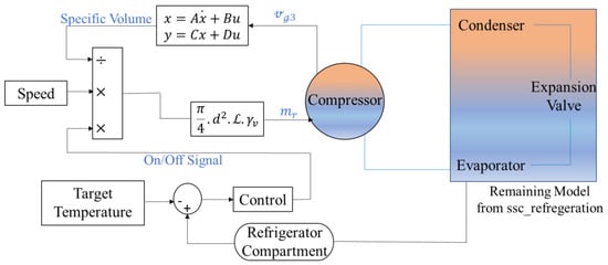
Figure 2.
SIMSCAPE thermal model of cooling process with reciprocating compressor.
2.3. Induction Motor (IM) Modeling
To develop the thermal-electric model of the cooling process, a model of an induction motor (IM) is needed. The in-built IM models of SIMSCAPE were considered for modeling the electrical characteristics of the three-phase induction motor. However, the models were too detailed for the CVR study because only the steady state behavior of motor was required, which is reached very quickly (in few seconds or less). Therefore, it was decided to use Equation (11) for modeling the torque vs. speed characteristics of the three-phase IM [23]. This equation neglects the magnetizing reactance because it is very large and has a negligible impact on the on-load performance of the IM. Solving (11) gives (13), which is the expression of . Equation (13) can be used with (12) to obtain the slip and hence the rotor speed. The IM model defined by (11)–(13) is shown in Figure 3.
where,
| electrical torque, mechanical torque | |
| synchronous angular speed of the rotor | |
| actual rotor speed | |
| voltage | |
| stator and rotor resistance, respectively | |
| stator and rotor reactance, respectively | |
| phases | |
| slip | |
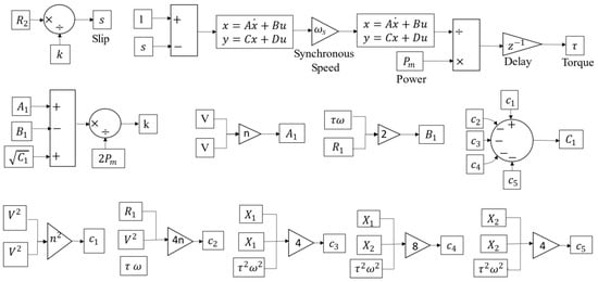
Figure 3.
Developed model for induction motor.
2.4. Thermal-Electric Model of Cooling Process
To develop the thermal-electric model of the cooling process, the compressor model of “ssc_refrigeration” was replaced by the compressor model of Figure 2 and the IM model of Figure 3. Adding the IM model resulted in algebraic loops being formed because the speed was being used to convert the compressor power into torque that was being input to the motor, while the torque was being used to obtain the rotor speed that was changing the refrigerant mass flow rate. To break this algebraic loop, a unit delay (1 s) was added. The detailed thermal-electric model of the cooling process is shown in Figure 4.
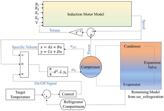
Figure 4.
Detailed thermal-electric model of cooling process.
3. Results and Discussion
Several simulations were performed using the models developed in the previous section. The data used for performing these simulations were primarily obtained from the “ssc_refrigeration” model discussed earlier, and they are given in Table 1. Additional data required for modeling the reciprocating compressor and three-phase IM are given in Table 2.

Table 1.
Parameters of ssc_refrigeration model.
Table 2.
Parameters of developed models.
Two scenarios were simulated using the thermal-electric model of Figure 4. The first scenario simulated conventional cooling equipment, where the compressor motor was driven directly from the utility power supply. In the second scenario, power electronics-based cooling equipment was considered, where the motor was assumed to be driven by a variable frequency drive (VFD) that is controlled using the widely used V/f control technique. Because the VFD decouples the motor power supply from the utility power supply, it is assumed that the controller can change the motor supply frequency according to the utility side voltage to maintain a constant V/f ratio. This is a reasonable assumption because making such changes to the VFD controllers is easy and only requires changes in the VFD firmware. Two sensitivities were also performed to evaluate the changes in the impact of CVR under different ambient and refrigerator target compartment temperatures.
For both simulation scenarios, the supply voltage varied between 90% to 110% of the rated voltage (220 V). All simulations were run for a duration of one day (86,400 s), and the data were recorded at a sampling rate of 1 Hz.
3.1. Base Results for Scenario 1 (Conventional Cooling Equipment)
The effect of voltage on the COP of the compressor and energy savings is shown in Figure 5. The results show that the COP increases on reducing the voltage. This is because the compressor speed reduces on reducing the supply voltage, due to which the input energy of the compressor decreases resulting in a higher COP. This effect, however, is negligible (maximum variation of 0.09%) because the change in speed over the entire voltage range is very small (24.8 Hz to 24.75 Hz or 0.9%).
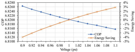
Figure 5.
Effect of voltage on COP and energy saving (pu stands for per unit and it is calculated in this paper as actual voltage divided by 220 V).
Contrary to the increase in the COP, the total energy consumption (total energy drawn from the supply, which is the sum of the compressor work and motor ohmic losses) of the cooling process increases as voltage is reduced compared to the rated voltage. This is shown in Figure 5 as the negative energy savings (total energy at the rated voltage minus total energy at a specified voltage) is expressed as a percentage of the total energy consumption at the rated voltage. This occurred because of the increase in motor ohmic losses (increased by 25% compared to losses at the rated voltage) when the voltage was reduced from rated to 90%. This observation aligns with the approximately constant power behavior of induction motors observed in practice, where reducing the voltage increases the current drawn at the same load, resulting in higher losses and reduced motor efficiency.
3.2. Base Results for Scenario 2 (Power Electronics-Based Cooling Equipment)
The effect of voltage on the COP of the compressor and energy savings is shown in Figure 6. In this simulation, the V/f ratio is kept constant, and the COP is observed by changing the voltage. The results show that the COP increases on reducing the voltage. This increase in the COP (about 4%) is around 40 times higher than the increase in the COP observed earlier for conventional cooling equipment (only 0.09%) when the voltage was reduced from 100% to 90%. This is because a decrease in the frequency to keep the V/f ratio constant results in a significantly higher reduction in motor speed (22.3 Hz) at reduced voltages compared to scenario 1, where the speed decreased to 24.75 Hz for the same change in utility voltage from the rated voltage to 90% of the rated voltage. In other words, the reduction in speed was 10% with respect to 25 Hz synchronous speed in scenario 2 (power electronics-based cooling equipment) while it was only 0.1% in scenario 1 (conventional cooling equipment). As a result, the compressor work reduces significantly more under the V/f control compared to conventional cooling equipment for the same voltage reduction.
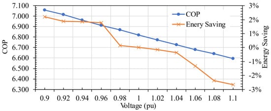
Figure 6.
Effect of Voltage on COP and Energy Saving (with V/f control).
Unlike the conventional case, energy savings are positive at voltages lower than the rated voltage. This is because the compressor work decreases by as much as 3% compared to without the V/f control, where the maximum reduction was 0.045%. At the same time, the increase in motor ohmic losses was significantly lower (maximum increase of 4% compared to losses at the rated voltage) than those observed in scenario 1 with conventional cooling equipment (maximum increase of 25% compared to losses at the rated voltage).
3.3. Sensitivity Results
Because of the very small impact of CVR on conventional cooling equipment, sensitivity results are provided only for scenario 2 with power electronics-based cooling equipment and V/f control.
3.3.1. Effect of Ambient Temperature on COP and Total Energy
The COP of the developed model is calculated by changing the ambient temperature from to in steps of and varying the voltage between 90% and 110%. The COP of the power electronics-based cooling equipment at different ambient temperatures with variations of voltage is given in Table 3. The table shows that, irrespective of the ambient temperature, the COP increases as the utility voltage is reduced. However, the COP of the power electronics-based refrigerator was very sensitive to changes in ambient temperature because the COP at 90% rated voltage decreased from 5.94 to 3.86 as the ambient temperature increased from to . The reduction in the COP at higher ambient temperatures can be explained by the higher heat ingress in the refrigerator compartment, thereby requiring the compressor to perform more work.
Table 3.
COP at different ambient temperature with variation of voltage.
Total energy consumption at different ambient temperatures is given in Table 4. The table shows that, irrespective of the ambient temperature, the total energy consumption decreases as the utility voltage is reduced. However, like the COP, the total energy consumption of the power electronics-based refrigerator was very sensitive to changes in ambient temperature because the total energy consumption at 90% rated voltage increased from 432.64 Wh to 1196.67 Wh as the ambient temperature increased from to .
Table 4.
Total energy consumption at different ambient temperature with variation of voltage.
3.3.2. Effect of Compartment Temperature on COP and Total Energy
In this sensitivity, the compartment temperature varied from to in steps of . The utility voltage again varied from 110% to 90% of the rated voltage. The COP values obtained from this sensitivity are shown in Table 5. While the trend of increasing COP at reduced voltages was observed at all compartment temperatures, the difference between the COPs at the simulated voltages reduced as the compartment temperature was reduced. In other words, the effect of CVR in improving the COP reduced as the compartment temperature was reduced.
Table 5.
COP at different compartment temperature with variation of voltage.
Similarly, the total energy consumption increased substantially as the compartment temperature was reduced but the reduction in total energy consumption at reduced voltages became much less as the compartment temperature decreased from to . For example, as shown in Table 6, the reduction in total energy consumption was 2.2% (at 90% rated voltage compared to the rated voltage) at the compartment temperature of 4, but this decreased to −0.6% (or the total energy increased slightly at 90% rated voltage compared to the rated voltage) when the compartment temperature was reduced to −8.
Table 6.
Total energy consumption at different compartment temperature with variation of voltage.
4. Experimental Validation
Hardware validation of the simulation results was performed at the Renewable Grid Integration Laboratory of the Department of Hydro and Renewable Energy at IIT Roorkee. The experimental setup is shown in Figure 7, and it is comprised of the following equipment:
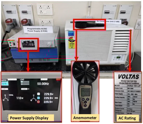
Figure 7.
Experimental setup.
- Programmable AC power supply: This was a 6 kVA, Kikusui make power supply (PCR6000WEA2), which acts like a grid except that it does not allow reverse power flow from equipment to the supply. Individual phase voltage magnitudes and phase angles and three-phase supply frequency can be precisely controlled. This feature was used to simulate the CVR and maintain the constant voltage to the frequency ratio. Moreover, the supply also displays power and current measurements, which were used to observe the power consumed by the air conditioner during experiments.
- Single-phase, conventional air conditioner: This was a Voltas window type air conditioner (Voltas 123 LZF) of 1000 W power rating, which acts as cooling equipment. The refrigerant used in this air conditioner is R32.
- Temperature sensor: Testo 417 vane anemometer was used to measure the fan speed and ambient temperature.
Experiments were performed for two scenarios, one for conventional cooling equipment and the other for power electronics-based equipment. The experimental setup is shown in Figure 7.
Two sets of the CVR experiments were performed. In one, only the supply voltage was reduced to 95% and 90% of the rated voltage of the air conditioner (230 V). In the second, the voltage to the frequency ratio was held constant as the voltage was reduced to 95% and 90% of the rated voltage. The wind speed of the fan and the room temperature were measured with the testo 417 vane anemometer. Each voltage level was maintained for 5 min and the steady value of power as displayed by the power supply was recorded.
In the simulation, only the compressor was modelled, whereas in the air conditioner a fan was also present. Therefore, to align the experiments with simulations, the power required by the air conditioner’s fan was subtracted from the total power displayed on the power supply to obtain the estimate for the compressor’s power consumption.
The average powers consumed by the compressor for the two sets of experiments are shown in Table 7 and Table 8, respectively. For the first set of experiments, where only the supply voltage was reduced, the power required by the compressor increased by 1.1% on reducing the voltage by 10%, whereas for the second set of experiments, where both voltage and frequency were reduced to keep their ratio constant, the power required by the compressor decreased by 5.07% on reducing the voltage by 10%.
Table 7.
Power saving with variation of voltage when only voltage was reduced.
Table 8.
Power saving with variation of voltage when both voltage and frequency were reduced to keep their ratio constant.
These results validate the trends observed in the simulations. The percentage increase or decrease in energy consumption was different because of the differences in the characteristics of the cooling equipment (single-phase motor, R34 refrigerant, and different and unknown thermal characteristics of the air conditioner) and the inability to control the ambient conditions because of the unavailability of a climate chamber with the research team.
5. Conclusions and Next Steps
Conservation Voltage Reduction (CVR) has been used by industries to save electricity by reducing incoming voltage. Many electricity distribution companies in the United States have also deployed CVR to reduce both peak power demand and the total energy use. Despite the long and successful experience with CVR programs, a physics-based modelling framework that could explain the key factors for energy savings by CVR and enable evaluation of CVR impacts in the future with changing end-use equipment, building technology, and deployment of distributed generation that can increase local voltages was missing.
This research attempted to address this gap by developing a thermal-electric model of cooling processes in MATLAB/SIMSCAPE and using it to demonstrate the efficacy of CVR programs under various conditions. Through these simulations, it was shown that it is difficult to generalize the effectiveness of CVR programs and attribute some fixed energy savings to CVR programs without performing detailed thermal-electric modeling of the facility and its equipment. It was found that for conventional, single speed compressors, contrary to the expectation, energy consumption (motor ohmic losses plus compressor work) increased by up to 4% as the voltage was reduced to 90% of the rated value. The trend of increased total energy consumption with reduced voltages (lower than the rated voltage) was also observed during compartment and ambient air temperature sensitivities.
The research performed has presented an intriguing opportunity of applying CVR on power electronics-based cooling equipment, which is rapidly increasing in our society. By appropriately modifying their control algorithms, the voltage–speed relationship can be changed to provide more impact of CVR (energy savings around 2.5%) than is possible in conventional cooling appliances (negative energy savings of 4%) that have limited speed range under normal operations.
These observations were also confirmed during hardware experiments, where only reducing the voltage while keeping the supply frequency fixed at 50 Hz resulted in an increase in energy (increase of 1.1% at 90% rated voltage and increase of 0.66% at 95% rated voltage when compared to the energy consumed at the rated voltage). However, when the ratio of the voltage and frequency was fixed, the energy consumption decreased by 5% and 2.6% at 90% and 95% rated voltages, respectively, when compared to the energy consumed at the rated voltage.
In the future, the authors intend to expand the thermal-electric model by including more detailed thermal models of buildings and electrical models of other appliances and equipment to observe the effect of CVR and quantify its effectiveness as an energy conservation strategy. Moreover, the authors intend to perform hardware validation of the impact of CVR using a climate-controlled chamber (not presently available with the research team), where the ambient temperature and humidity can be precisely controlled.
Author Contributions
Conceptualization: H.J.; methodology, H.J., H.V. and R.T.; investigation, H.V., R.T. and H.J.; writing—original draft preparation, H.V., R.T. and H.J.; writing—review and editing, H.J. and H.V.; visualization, H.V. All authors have read and agreed to the published version of the manuscript.
Funding
This research received no external funding.
Institutional Review Board Statement
Not applicable.
Informed Consent Statement
Not applicable.
Data Availability Statement
The data required to run the simulations performed in this study is provided within the body of the paper. The data analyzed here is available on request.
Conflicts of Interest
The authors declare no conflict of interest.
References
- Energy Efficiency Impact Report—Why Energy Efficiency Matters. Available online: https://energyefficiencyimpact.org/ (accessed on 8 January 2023).
- Kamat, A.S.; Khosla, R.; Narayanamurti, V. Illuminating homes with LEDs in India: Rapid market creation towards low-carbon technology transition in a developing country. Energy Res. Soc. Sci. 2020, 66, 101488. [Google Scholar] [CrossRef]
- The Paris Agreement|UNFCCC. Available online: https://unfccc.int/process-and-meetings/the-paris-agreement/the-paris-agreement (accessed on 8 January 2023).
- Chen, M.S.; Shoults, R.; Fitzer, J.; Songster, H. The effects of reduced voltages on the efficiency of electric loads. IEEE Trans. Power Appar. Syst. 1982, PAS-101, 2158–2166. [Google Scholar] [CrossRef]
- Kennedy, B.W.; Fletcher, R.H. Conservation voltage reduction (CVR) at snohomish county PUD. IEEE Trans. Power Syst. 1991, 6, 986–998. [Google Scholar] [CrossRef]
- Bokhari, A.; Alkan, A.; Dogan, R.; Diaz-Aguiló, M. Experimental determination of the ZIP coefficients for modern residential, commercial, and industrial loads. IEEE Trans. Power Deliv. 2014, 29, 1372–1381. [Google Scholar] [CrossRef]
- Diaz-Aguiló, M.; Sandraz, J.; Macwan, R.; De Leon, F.; Czarkowski, D.; Comack, C.; Wang, D. Field-validated load model for the analysis of CVR in distribution secondary networks: Energy conservation. IEEE Trans. Power Deliv. 2013, 28, 2428–2436. [Google Scholar] [CrossRef]
- Paul, S.; Jewell, W. Impact of load type on power consumption and line loss in voltage reduction program. In Proceedings of the 2013 North American Power Symposium (NAPS), Manhattan, KS, USA, 22–24 September 2013. [Google Scholar] [CrossRef]
- Singaravelan, A.; Kowsalya, M. A Practical Investigation on Conservation Voltage Reduction for its Efficiency with Electric Home Appliances. Energy Procedia 2017, 117, 724–730. [Google Scholar] [CrossRef]
- Wang, Z.; Wang, J. Review on implementation and assessment of conservation voltage reduction. IEEE Trans. Power Syst. 2014, 29, 1306–1315. [Google Scholar] [CrossRef]
- Schneider, K.P.; Fuller, J.C.; Chassin, D.P. Multi-state load models for distribution system analysis. IEEE Trans. Power Syst. 2011, 26, 2425–2433. [Google Scholar] [CrossRef]
- Kampezidou, S.; Wiegman, H. Energy and power savings assessment in buildings via conservation voltage reduction. In Proceedings of the 2017 IEEE Power and Energy Society Innovative Smart Grid Technologies Conference, ISGT 2017, Washington, DC, USA, 23–26 April 2017. [Google Scholar] [CrossRef]
- El-Shahat, A.; Haddad, R.J.; Alba-Flores, R.; Rios, F.; Helton, Z. Conservation voltage reduction case study. IEEE Access 2020, 8, 55383–55397. [Google Scholar] [CrossRef]
- Sunderman, W.G. Conservation voltage reduction system modeling, measurement, and verification. In Proceedings of the PES T&D 2012, Orlando, FL, USA, 7–10 May 2012. [Google Scholar] [CrossRef]
- Two-Phase Fluid Refrigeration—MATLAB & Simulink—MathWorks India. Available online: https://in.mathworks.com/help/simscape/ug/two-phase-fluid-refrigeration.html;jsessionid=e45a89a857a5384060dc04f30bac (accessed on 8 January 2023).
- Incropera, F.P.; DeWitt, D.P.; Bergman, T.L.; Lavine, A.S. Fundamentals of Heat and Mass Transfer, 6th ed.; Wiley: Hoboken, NJ, USA, 2007. [Google Scholar]
- Çengel, Y.A.; Boles, M.A. Thermodynamics: An Engineering Approach, 7th ed.; McGraw-Hill: New York, NY, USA, 2011. [Google Scholar]
- Macagnan, M.H.; Copetti, J.B.; De Souza, R.B.; Reichert, R.K.; Amaro, M. Analysis of the Influence of Refrigerant Charge and Compressor Duty Cycle in an Automotive Air Conditioning System. In Proceedings of the 22nd International Congress of Mechanical Engineering (COBEM 2013), Ribeirão Preto, SP, Brazil, 3–7 November 2013. [Google Scholar]
- Arthur, J.H.; Beard, J.T.; Bolton, C. Simplified analytical modeling of an air conditioner with a positive displacement compressor. In Proceedings of the Intersociety Energy Conversion Engineering Conference, Washington, DC, USA, 11–16 August 1996; Volume 3, pp. 2009–2014. [Google Scholar] [CrossRef]
- Liu, Y.; Vittal, V.; Undrill, J.; Eto, J.H. Transient model of air-conditioner compressor single phase induction motor. IEEE Trans. Power Syst. 2013, 28, 4528–4536. [Google Scholar] [CrossRef]
- Jie, D. Modeling and Simulation of Temperature Control System of Coating Plant Air Conditioner. Procedia Comput. Sci. 2017, 107, 196–201. [Google Scholar] [CrossRef]
- Negrao, C.O.; Erthal, R.; Andrade, D.E.; Silva, L. An Algebraic Model for Transient Simulation of Reciprocating Compressors. International Compressor Engineering Conference. January 2010. Available online: https://docs.lib.purdue.edu/icec/2032 (accessed on 30 March 2023).
- Umans, S.D.; Fitzgerald, A.E. Fitzgerald & Kingsley’s Electric Machinery; McGraw-Hill Companies: New York, NY, USA, 2014; p. 706. [Google Scholar]
- Compressor Model GS26TB_T 220-240V 50Hz ~ 1 Refrigerant. Technical Data Sheet. Available online: https://lightcommercialrefrigeration.danfoss.com/pdf/danfoss_GS26TB_T_R134a_220_50.pdf (accessed on 30 March 2023).
- Lin, S.; He, Z.; Guo, J. Study of aerodynamic noise in hermetic refrigerator compressor. In Proceedings of the 8th International Conference on Compressors and Their Systems, London, UK, 9–10 September 2013; Institution of Mechanical Engineers: London, UK, 2013; pp. 397–403. [Google Scholar] [CrossRef]


Disclaimer/Publisher’s Note: The statements, opinions and data contained in all publications are solely those of the individual author(s) and contributor(s) and not of MDPI and/or the editor(s). MDPI and/or the editor(s) disclaim responsibility for any injury to people or property resulting from any ideas, methods, instructions or products referred to in the content. |
© 2023 by the authors. Licensee MDPI, Basel, Switzerland. This article is an open access article distributed under the terms and conditions of the Creative Commons Attribution (CC BY) license (https://creativecommons.org/licenses/by/4.0/).