Space Cooling Energy Potential of Domestic Cold Water before Household Consumption in Cold-Climate Regions

Abstract

Space cooling energy consumption in residential buildings has tripled globally over the past three decades, leading to a significant increase in greenhouse gas (GHG) emissions and building operating costs. To reduce building cooling energy consumption, cooling energy can be recovered from domestic cold water (DCW) for space cooling by circulating DCW through thermally massive walls (herein “DCW-wall”) before regular household consumption (e.g., showers). This approach is more effective in cold climate regions since the DCW is cooler in these regions, yet its engineering design and effectiveness have not been evaluated previously. This study evaluated the cooling potential of DCW-walls in different operation scenarios (e.g., inlet temperatures, zone temperatures, and piping configurations). A typical DCW usage pattern and a daily amount of 1200 L were selected for evaluation. Three-dimensional transient thermal simulations were used to obtain the water outlet temperatures, average wall surface temperatures, and cooling potentials. The results showed that a DCW wall with a spiral piping configuration and DCW inlet at 12 °C can deliver 21.92 MJ of cooling energy daily to a zone at 25 °C. This amount of free energy can cover up to approximately 11% of the annual cooling energy demand of a four-person dwelling in Toronto, Canada, which has a warm and humid summer.

1. Introduction

Buildings account for 30–40% of the world’s total energy expenditure, as well as 20–30% of total global greenhouse gas (GHG) emissions [1,2]. The European Union (EU-28) saw an average annual increase of 6.3% in space cooling energy consumption from 2000 to 2015 [3]. Adopting energy-efficient measures, such as free cooling techniques, effectively reduces a building’s energy consumption. [4,5,6]. One such technique is ventilative cooling, which utilizes ambient air for space cooling [7,8]. Although ventilative cooling can reduce energy consumption, its overall effectiveness is hampered by certain limitations. For example, during heat waves, outdoor temperatures may not be cool enough [9]. Cooling energy recovery from cold water can offer a substantial amount of free cooling. A 10 °C change in water temperature and a daily water consumption of 1000 L produces approximately 42 MJ of free cooling energy. A recent application is the cooling of subway stations and shelters during heat waves [10]. Furthermore, past studies have examined the effect of cold recovery from domestic cold water (DCW) on GHG emissions, financial considerations, and water quality [11,12,13].

To recover cooling energy from DCW, DCW can be circulated through pipes embedded in a thermally massive wall before it is dispensed by occupants for regular domestic usage. Hydronic panel heating and cooling systems have extensively employed thermally massive building components, such as concrete walls and floors [14]. These systems are often referred to as thermally activated building systems (TABS). TABS reduces space heating/cooling energy consumption and mechanical system capacities through thermal energy storage (TES) [15,16,17,18]. TES stabilizes cooling heat flux (i.e., cooling capacity) fluctuations and wall surface temperature, preventing the surface temperature from falling too quickly to extremely low values. Massive walls are preferable to metal panels since the former can store higher amounts of thermal energy, prevent excessive low wall surface temperature, and elongate the cooling period. TABS also enhances thermal comfort by creating a gradual change in indoor air temperature and evenly distributing the heat flux density [19].

Several research studies have been conducted to identify the key parameters that affect the cooling performance of TABS. In a parametric study, Antonopoulos et al. [20] determined that water inlet temperature, pipe spacing, pipe depth, and zone air temperature had significant effects on thermal performance, while other parameters had a negligible impact. These observations have been confirmed by similar studies [21,22,23]. The water cooling capacity (i.e., how well the water removes heat from the wall) and wall surface cooling capacity (i.e., how well the wall removes heat from the associated zone) in hydronic pipe-embedded systems are significantly influenced by the supply water temperature. Antonopoulos et al. [20] discovered that lowering the supply water temperature from 15 °C to 5 °C resulted in an increase in cooling heat flux density from 45 W/m² to 120 W/m². Furthermore, different studies have also investigated the use of relatively high-temperature water (18 °C to 25 °C) for space cooling to reduce energy consumption. Šimko et al. [24] conducted an experiment to determine the maximum cooling capacity for a 16 °C to 25 °C water inlet temperature range. Similar studies [25,26,27] carried out experiments with a supply water temperature range of 18 °C to 21 °C. Raising water supply temperatures would lead to a reduction in energy consumption for chilling water. However, it would also result in a notable decrease in the cooling capacity of the TABS system [19]. Moreover, further studies [21,26,28] have demonstrated that pipe spacing significantly affects cooling capacity. They found that decreasing the pipe spacing in the same area would result in greater cooling capacity due to an increase in the heat transfer area. Junasová et al. [29] discovered that by reducing the pipe spacing from 15 cm to 5 cm, the cooling capacity increased by over 40%.

Using thermally massive walls to recover cooling energy from DCW (herein as “DCW-wall”) and assist space cooling does not require complex construction. A diverter valve can be installed to allow DCW to bypass the massive walls during the heating season. Therefore, DCW-walls could potentially reduce capital and operating costs compared with other space cooling technologies due to lower installation costs, downsizing, and ultimately the potential elimination of mechanical cooling systems and their maintenance requirements [30,31,32]. In cold regions such as Canada, where the ground temperature is relatively lower than other regions, more cooling energy can be recovered. In addition, the outlet temperature of DCW will be warmed by room air to make it more suitable for domestic usage (e.g., less mixing with domestic hot water in showers).

The existing literature predominantly focuses on space cooling using chilled water provided by mechanical equipment. However, the authors have observed a research gap in the evaluation of the free cooling potential of DCW before it is used for regular household consumption while also taking into account actual water consumption patterns in residential buildings. Therefore, the primary focus of this study is to address the question: “What is the cooling potential and energy-saving effectiveness of using DCW for space cooling through DCW-walls in residential buildings located in cold-climate regions?” The objective of this paper is to investigate the effectiveness of circulating DCW through thermally massive walls before regular household consumption. Through a comprehensive evaluation of various operational scenarios, such as inlet temperatures, zone temperatures, and engineering designs, this study aims to quantify the range of cooling potential achievable with DCW-walls. Specifically, the focus is on cold climate regions where DCW is relatively cooler, as this presents an opportunity for enhanced energy recovery. Additionally, this study will assess the extent to which the daily cooling energy supplied by a DCW-wall can meet the annual cooling energy requirements of a four-person dwelling in Toronto, Canada, which experiences warm and humid summers.

In terms of the paper’s organization, the research methodology is discussed first, followed by the development and validation of the numerical model. Then, the following Section 3 has six subsections discussing water outlet temperature, average wall temperature, temperature uniformity, condensation prevention, cooling capacity, delivered (recovered) cooling energy (DCE), the performance difference of the three piping configurations, and the influence of wall surface area on total DCE.

2. Methodology

A zone temperature is the main boundary parameter that influences the cooling performance of a DCW-wall if direct solar radiation on the wall is not present. Running whole building thermal simulations can provide such a zone temperature profile and the corresponding DCW-wall performance; however, this approach will only provide the performance for the chosen specific building characteristics (e.g., physical construction, room temperature settings, and location of the DCW-wall) and climate conditions. This study aims to generalize the performance of DCW-walls by providing a performance envelope for DCW-walls through a parametric analysis. Zone temperature is included as one of the parameters, thereby avoiding time-consuming, case-specific whole-building thermal simulations. By estimating the performance of a DCW-wall based on a range of zone temperatures, the performance can be interpreted for a broader range of zone conditions. The following sections describe the physical system, the selected DCW flow pattern, and the numerical model and its configurations used for parameter analysis.

2.1. Description of the Physical System

Figure 1 shows the DCW-wall system. In this system, DCW is routed through copper pipes embedded in the middle layer of a thermally massive wall to cool the zone by exchanging heat with a warm indoor environment. The outlet water is directed to the dispensers for regular household use. The dispensers depicted in Figure 1 serve as illustrative examples of different types of dispensers to which the outlet pipe can be connected, even though the connections are not shown. A diverter valve can be installed to allow the DCW to bypass the wall in space heating months. The wall considered in this study is an exterior wall, with one side being exposed to the indoor zone air.

Figure 2 shows copper pipes embedded in the middle layer of a wall in three different patterns: spiral, serpentine, and parallel. The length of the pipe required for each configuration varies based on the spacing (M) of the pipes and the dimensions of the wall. The ASHRAE [33] recommends pipe spacing for radiant heating and cooling systems to be between 10 cm and 30 cm. A pipe spacing of 10 cm is recommended by [22,25] in order to maximize the cooling capacity of the system. This was supported by a study [21], in which they compared the cooling capacity of the system at two different pipe spacings of 10 cm and 30 cm. The present study demonstrated that, using a pipe spacing of 10 cm in a 2 m × 3 m wall, the total length of pipe required for spiral, serpentine, and parallel patterns were 56 m, 58 m, and 57 m, respectively. Similarly, when using a pipe spacing of 30 cm, the total length of the pipe used in spiral, serpentine, and parallel patterns was 22 m, 23 m, and 18 m, respectively.

2.1.1. Variable DCW Flow

Households have a relatively similar daily pattern of water consumption regardless of the total amount of water consumption [34]. Figure 3 shows a typical daily pattern of average hourly water consumption for residential buildings in Australia [35,36]. The hourly values correspond to the average values of families of four, for a total of 1200 L of water flowing per day [13]. The maximum flow rate is 0.03 L/s at 7 a.m. Two peak hours can be observed: one in the morning and the other in the evening. The flow rate gradually decreased from 5 p.m. to 3 a.m. the following day, eventually reaching near zero. The thermal models presented in this paper use the variable DCW flow and assume it is steady periodic with a cycle of 24 h.

2.1.2. Numerical Model

The following configurations were incorporated into the thermal models:

• In cold climate regions, such as Canada, municipal domestic water lines are buried around 1.5 to 2 m deep in the ground. Therefore, the temperature of domestic water entering households is similar to the ground temperature at these depths. Two water inlet temperatures ($T_{\mathrm{S}\mathrm{W}}^{}$) of 12 °C and 15 °C were selected based on the mean monthly ground temperatures in the summer (June to August) in Toronto, Canada [37]. Two fixed zone temperatures ($T_{\mathrm{a}\mathrm{i}\mathrm{r}}^{}$) of 25 °C and 30 °C were used for thermal simulations.
• A temperature of 26 °C is considered a safe threshold for an indoor environment [38]. In this context, an increase in emergency medical calls and premature mortality rates has been associated with indoor temperatures above 26 °C [39]. In addition, heat warnings are usually issued when maximum daily temperatures reach 30 °C in Canada [39]. The zone temperature is likely to reach 30 °C in the heat warning periods without mechanical cooling. Therefore, in this study, zone temperatures ($T_{\mathrm{a}\mathrm{i}\mathrm{r}}^{}$) of 25 °C and 30 °C are used as the lower and upper limits of the zone temperature during cooling seasons. The results obtained based on these two fixed zone temperatures represent the performance envelope of the DCW-walls. It offers a range for the cooling potential of the DCW-wall for zone temperatures between 25 °C and 30 °C.
• The dimensions of the modeled wall are 2 m in height and 3 m in width. The impact of different wall areas on the total DCE will be discussed in Section 3.6. Furthermore, the simulations were conducted with two wall thicknesses of 5 cm and 10 cm to assess the impact of TES on cooling potentials and wall temperature.
• The exterior side of the DCW-wall is assumed to be adiabatic because of the thick thermal insulation used in cold-climate buildings, and the temperature difference between the wall and the exterior is not significant during a cooling season.
• As discussed above, pipe spacings of 10 cm and 30 cm were used to determine the cooling potentials of the DCW-wall system. In this paper, the results are presented for both the top and bottom of the optimal spacing range. The pipe was placed in the middle layer of the wall.
• The temperature of each control volume of the water or wall is assumed to be uniform. Temperature nodes were placed at the center of each control volume.
• The convective thermal resistance between the water and the pipe ($h_{\mathrm{w}\mathrm{a}\mathrm{t}\mathrm{e}\mathrm{r}}^{}$) was considered in all thermal models.
• Under a steady-periodic daily water flow pattern and constant boundary conditions, transient thermal simulations were conducted. When the temperature profiles stabilized (i.e., the temperatures of all control volumes converged), the results of the last 24-h period were used for analysis.

Using the method of rectangular control volumes [40], a 3D numerical model was developed to analyze the cooling potentials of using DCW as a cooling medium in a thermally activated wall system in cold-climate residential buildings. Figure 4 depicts a 3D schematic of the wall, which includes temperature nodes, control volumes (CVs), and the thermal transmittances between a water node and its adjacent wall node. X-Step, Y-Step, and Z-Step refer to the distances between the two nodes in the x, y, and z directions, respectively. The X-Step and Y-Step were set at 5 cm, but the Z-Step can be equal or unequal for different layers along the thickness, depending on the objectives or required accuracy for thermal simulations or model validation. For this study, the number of layers for the 5 cm- and 10 cm-thick walls was one and three, respectively, with unequal Z-Step used in the latter. The control volumes have a length (x-direction) and height (y-direction) of 5 cm. The width (z-direction) of each control volume varies based on the thickness of the wall. For a wall thickness of 5 cm, the width is equal to the thickness itself (i.e., 5 cm). However, when the wall thickness is set at 10 cm, the wall is divided into three layers. The first layer (surface) and the middle layer (where the pipe is located) have a width of 2.5 cm each, while the third layer (back of the wall) has a width of 5 cm.

Water Nodes

Water temperature can be obtained using Equation (1) [40], which can be discretized into a finite difference equation and solved explicitly [41].

$$\begin{gathered} {\left(\mathrm{\rho }\mathrm{C}\mathrm{p}\right)}_{\mathrm{w}\mathrm{a}\mathrm{t}\mathrm{e}\mathrm{r}}\left(\pi \frac{{\mathrm{D}}_{\mathrm{i}}^2}{4}\times L_f\right)\frac{d{T}_{\mathrm{w}\mathrm{a}\mathrm{t}\mathrm{e}\mathrm{r}}^{\mathrm{f}}}{dt}=U_p\left(T_{wall}^{i,j,k}-T_{\mathrm{w}\mathrm{a}\mathrm{t}\mathrm{e}\mathrm{r}}^{\mathrm{f}}\right)-\dot{m}{\mathrm{C}\mathrm{p}}_{\mathrm{w}\mathrm{a}\mathrm{t}\mathrm{e}\mathrm{r}}\left(T_{\mathrm{w}\mathrm{a}\mathrm{t}\mathrm{e}\mathrm{r}}^{\mathrm{f}}-T_{\mathrm{w}\mathrm{a}\mathrm{t}\mathrm{e}\mathrm{r}}^{\mathrm{f}-1}\right) \\ f=\mathrm{1,2},3,\dots ,{\mathrm{n}}_{\mathrm{p}\mathrm{i}\mathrm{p}\mathrm{e}} \end{gathered}$$

(1)

where ${\mathrm{\rho }}_{\mathrm{w}\mathrm{a}\mathrm{t}\mathrm{e}\mathrm{r}}$ and ${\mathrm{C}\mathrm{p}}_{\mathrm{w}\mathrm{a}\mathrm{t}\mathrm{e}\mathrm{r}}$ are the density and specific heat capacity of the water, respectively. ${\mathrm{D}}_{\mathrm{I}}^{}$ and $L_f$ denote the inside diameter of the pipe and the length of the CV that corresponds to node $f$ on the pipe in the direction of the water flow, respectively. Indices $i,j,k$, and $f$ represent the node counter for the wall in three directions and the pipe in the direction of the water flow. In Equation (2), $i,j,k$ are the node coordinates of the wall CV that are in contact with node $f$ of the pipe. $T_{\mathrm{w}\mathrm{a}\mathrm{l}\mathrm{l}}^{}$, $T_{\mathrm{w}\mathrm{a}\mathrm{t}\mathrm{e}\mathrm{r}}^{}$, $\dot{m}$, and $U_p$ denote the wall temperature and water temperature in their respective CVs, the water mass flow rate, and the total thermal transmittance between the water node and adjacent wall node, respectively. Equation (2) can be used to calculate the $U_p$.

$$U_p=\frac{1}{\frac{1}{U_{\mathrm{P}1}^{}}+\frac{1}{U_{\mathrm{P}2}^{}}+\frac{1}{U_{\mathrm{P}3}^{}}}$$

(2)

As illustrated in Figure 4; $U_{\mathrm{P}1}^{}$, which is the total thermal transmittance between water and the pipe; $U_{\mathrm{P}2}^{}$, which is the total thermal transmittance between the inner and outer surfaces of the pipe; and $U_{\mathrm{P}3}^{}$, which is the total thermal transmittance between the cylindrical pipe’s surface and the adjacent wall node. $U_{\mathrm{P}3}^{}$ considers the shape factor for the accurate calculation of heat energy exchange between a circular cylinder (i.e., pipe) centered in a solid square (i.e., control volumes) [41]. More details on calculating the thermal transmittances of $U_{\mathrm{P}1}^{}$, $U_{\mathrm{P}2}^{}$, and $U_{\mathrm{P}3}^{}$ can be found in Appendix A.

Wall Nodes

The wall temperature at any given location (i.e., node) can be determined using Equation (3).

$${\left(\mathrm{\rho }\mathrm{C}\mathrm{p}\right)}_{\mathrm{w}\mathrm{a}\mathrm{l}\mathrm{l}}{V}_{wall}^{i,j,k}\frac{d{T}_{wall}^{i,j,k}}{dt}=Q_{w2w}^{i,j,k}+Q_{surface}^{i,j,k}+Q_{conduction}^{i,j,k}$$

(3)

where $V_{wall}^{}$ is the volume of each CV, $Q_{w2w}^{}$ denotes the heat flux between water and wall which is positive, $Q_{surface}^{}$ represents the heat flux from the zone towards the wall nodes which is positive at the stated direction, and $Q_{conduction}^{}$ is the conduction heat transfer between the wall nodes, which can be calculated using Equation (4).

$$Q_{conduction}^{i,j,k}={\mathrm{\lambda }}_{\mathrm{w}\mathrm{a}\mathrm{l}\mathrm{l}}\times \left\{\begin{array}{c}\frac{∆z∆\mathrm{y}}{∆\mathrm{x}}\left(T_{wall}^{i+1,j,k}+T_{wall}^{i-1,j,k}-{2T}_{wall}^{i,j,k}\right)\\ +\frac{∆z∆\mathrm{x}}{∆\mathrm{y}}\left(T_{wall}^{i,j+1,k}+T_{wall}^{i,j-1,k}-{2T}_{wall}^{i,j,k}\right)\\ +\frac{∆\mathrm{y}∆\mathrm{x}}{∆z}\left(T_{wall}^{i,j,k+1}+T_{wall}^{i,j,k-1}-{2T}_{wall}^{i,j,k}\right)\end{array}\right\}$$

(4)

where ∆x, ∆y, and ∆z stands for the x-direction, y-direction, and z-direction length of each CV, respectively.

Table 1. Values for some parameters in three layers of the DCW-wall.

Wall Thickness	Layer	${\mathit{Q}}_{\mathit{w}2\mathit{w}}^{}$	${\mathit{Q}}_{\mathit{s}\mathit{u}\mathit{r}\mathit{f}\mathit{a}\mathit{c}\mathit{e}}^{}$	${\mathit{V}}_{\mathit{w}\mathit{a}\mathit{l}\mathit{l}}^{\mathit{i},\mathit{j},\mathit{k}}$
10 cm	Front	0	$U_{int}(T_{air}^{}-T_{wall}^{i,j,k})$	$∆z\times ∆x\times ∆y$
	Middle	$U_p(T_{wall}^{i,j,k}-T_{water}^f)$	0	($∆z\times ∆x\times ∆y)-(\pi \frac{D_o^2}{4}\times L_f)$
	Back	0	0	$∆z\times ∆x\times ∆y$
5 cm	-	$U_p(T_{wall}^{i,j,k}-T_{water}^f)$	$U_{int}(T_{air}^{}-T_{wall}^{i,j,k})$	($∆z\times ∆x\times ∆y)-(\pi \frac{D_o^2}{4}\times L_f)$

shows the value of $Q_{w2w}^{}$, $Q_{surface}^{}$, and $V_{wall}^{}$ for the layers along the wall thickness. A wall with a thickness of 10 cm consists of 3 layers, while a wall with a thickness of 5 cm has only one layer.

where $U_{int}$ is the total thermal transmittance between the wall surface and the zone air. $U_{int}$ can be obtained using Equation (5).

$$U_{int}=h_{total}\times ∆y\times ∆x$$

(5)

$h_{total}$ is the combined heat transfer film coefficient between the wall surface and the zone air. A constant value of 9.09 W/m²·K was used for $h_{total}$ in the model because the air speed inside the zone was assumed to be low. As a result, $h_{total}$ was not subjected to substantial variation [33,42].

2.1.3. Model Validation

Merabtine et al. [43] conducted an experimental study on the thermal characteristics of floor heating systems. In their study, the floor had a configuration similar to the wall modeled in this study. From top to bottom, the floor consisted of anhydrite concrete screed (4 cm), polyethylene raised temperature resistance (PE-RT) pipes embedded in the screed in a spiral pattern, and polyurethane insulation (5.6 cm). All specifications mentioned in the experimental study were considered by modifying the numerical model parameters using those proposed in the experiment. Among these specifications were transient water inlet and zone temperatures, water flow rate, pipe material, pipe spacing, piping pattern, floor dimensions, floor thickness, and the precise location of the pipes embedded in the floor. The average floor surface temperature was measured every 10 min for 5 h. Figure 5 illustrates the changes in the measured and simulated average floor surface temperatures. The coefficient of variation of the root-mean square error (CV-RMSE) statistical measure was chosen to represent the error between the simulated and measured values. The CV-RMSE was calculated by dividing the root mean square error by the average of the measured data. CV-RMSE was determined using Equation (6) [44].

$$CV-RMSE=\frac{\sqrt{\frac{\sum _{i=1}^n{(y_i-\widehat{y_i})}^2}{n}}}{\overline{y}}$$

(6)

where $n$ is the number of data points; $y_i$ is the measured value; $\widehat{y_i}$ is the simulated value; and $\overline{y}$ is the average of all measured values. In comparison to the experimental study’s measured values, the current study exhibits a CV-RMSE value of 1.5%.

3. Results and Discussion

This section presents the main results and associated analyses. For better clarity, the performance of the spiral configuration is presented first in the first four subsections: Section 3.1—water outlet and average wall temperatures, Section 3.2—wall surface temperature uniformity and a general guideline for preventing condensation on the wall, Section 3.3—cooling heat flux density, and Section 3.4—delivered cooling energy, based on the following parameters:

• Supply water temperature ($T_{SW}$),
• Zone temperature ($T_{air}$),
• Wall thickness ($S$),
• Pipe spacing ($M$).

Section 3.5 compares the performance of the three configurations in the same above-mentioned aspects. The descriptions and figures in these subsections are for the temperature scenario of $T_{SW}$ = 12 °C, $T_{air}$ = 25 °C, and $S$ = 5 cm. The results for cooling heat flux density and delivered cooling energy of the other temperature scenarios, and wall thickness are tabulated in Section 3.5. Section 3.6 presents the influence of the wall surface area on the delivery cooling energy.

3.1. Water Outlet and Average Wall Temperatures

The behavior of the wall surface temperature varies depending on the system configuration. It is essential to calculate the surface temperature of the wall because the cooling capacity of the system is directly influenced by the temperature difference between the wall surface and the zone. In addition, calculating the minimum wall temperature is critical to determining the minimum allowable humidity level of the zone air to avoid condensation on the wall surface. Condensation also reduces the effectiveness of radiant cooling systems [45]. Moreover, thermal comfort can be impacted by the uniformity of the surface temperature. Figure 6 shows the average surface temperature fluctuations for a spiral configuration over a 24-h period.

The average wall surface temperature reaches its lowest values approximately 2 to 3 h after the water flow rate reaches its highest values, as shown in Figure 6. The average surface temperature dropped to 19 °C and 20.6 °C at 19:00 for spacings of $M$ = 10 cm and $M$ = 30 cm, respectively. The 10 cm-thick wall is 1 °C less than the 5 cm-thick wall in this situation. As the flow rate approached zero, the surface temperature was close to the zone temperature due to insignificant heat rejection from the wall to the pipe. At the same time, the wall absorbed a significant amount of heat from the zone. Conversely, with an increase in the water flow rate, the wall surface temperature decreases because of a greater heat flux from the wall to the water, which leads to an increase in the water outlet temperature. The temperature range for the water outlet in both spacings of the spiral configuration varied between 16.7 °C and 24.2 °C. Figure 7 shows the water outlet temperature variation for the spiral counterflow configuration.

3.2. Temperature Uniformity and Condensation Prevention

Temperature distribution on the wall surface is crucial not only for the comfort of the occupants but also for reducing the risk of condensation [46,47]. Figure 8 plots the wall surface temperature along the water flow path versus its distance from the water inlet and time of day for the spiral configuration. The coldest temperature is always at the inlet. The warmed temperature takes place between 3 AM and 6 AM at the pipe distance between 20 to 45 m from the inlet, which is at the center of the wall surface. Figure 8 shows a maximum surface temperature difference of 3.5 °C across the wall at a pipe spacing of 10 cm and a difference of 3 °C at 30 cm.

To avoid condensation, the minimum wall surface temperature should be higher than the dewpoint temperature of the air inside the zone. To establish a conservative yet simple guideline, two minimum wall surface temperatures of all operation scenarios were used as dewpoint temperatures. Thereby, the corresponding relative humidity (RH) is found from a psychrometric chart based on the zone air temperature, as shown in

Table 2. Allowable indoor RH to prevent condensation in spiral configuration.

${\mathit{T}}_{{\mathit{w}\mathit{a}\mathit{l}\mathit{l}.\mathit{m}\mathit{i}\mathit{n}}_{}}$$/{\mathit{T}}_{\mathit{a}\mathit{i}\mathit{r}}$ (°C)	Allowable RH (%)
15/25	≤53.8
16.5/30	≤44.2

. To avoid condensation on the wall surface, indoor RH should not exceed 53.8% and 44.2% when the zone temperature is 25 °C and 30 °C, respectively. These findings are in agreement with the ideal indoor RH, which is between 30% and 50% [48].

3.3. Cooling Heat Flux Density

In this study, the amount of heat absorbed by the wall surface from the zone per square meter of wall (W/m²) is referred to as the cooling heat flux density (i.e., cooling capacity). Cholewa et al. [49,50] argued that due to heat loss toward the backside of cooled/heated walls, calculations of cooling capacity based on water temperature and flow rate do not always accurately represent the heat flux toward the zone. Cooling capacity can be obtained using Equation (7). According to this equation, the cooling capacity (q) is always positive when cooling is delivered to the zone air (i.e., the zone air temperature is higher than the average wall surface temperature).

$$q=h_{total}(T_{air}-T_{wall})$$

(7)

The combined heat transfer coefficient ($h_{total}$) between the zone and wall surface was set to 9.09 W/m²·K [33]. Figure 9 shows the changes in cooling capacity for the spiral configuration over a 24-h period.

As shown in Figure 9, the cooling capacity reached its maximum at 50 W/m² for $M$ = 10 cm and at 35.0 W/m² for $M$ = 30 cm. The cooling capacity for $M$ = 10 cm was significantly higher than that for $M$ = 30 cm. This can be attributed to the longer pipe length, which provided a larger heat transfer area and a more uniform surface temperature, resulting in fewer hot spots. For both spacings, the minimum cooling capacity was around 10 W/m² when the flow rate was almost zero.

3.4. Delivered Cooling Energy

The delivered cooling energy (DCE) in this study was defined as the amount of cooling energy from the water delivered to the room and the wall (i.e., heat loss from the water flow) and was calculated using Equation (8).

$$E_{DCE}=\dot{m}{Cp}_{\mathrm{w}\mathrm{a}\mathrm{t}\mathrm{e}\mathrm{r}}\left(T_{ow}\left(t\right)-T_{sw}\right)∆t$$

(8)

where $∆t$ is the simulation timestep (i.e., 60 s).

Figure 10 illustrates the cumulative DCE (“Total DCE”), the portion of DCE that goes to the room (“DCE to room”), and the amount of energy stored in the wall (“Energy stored in wall”) during a 24-h period.

DCE to room equals the amount of heat transferred between the room and the surface of the wall. Furthermore, the energy stored in the wall is calculated based on the difference between the total DCE and the DCE to room, which can either be heat storage (i.e., the wall temperature increases, negative values in Figure 10) or cold storage (i.e., wall temperature decreases, positive values in Figure 10). As shown in Figure 10, in the first five hours, the accumulated energy stored in the wall (“Energy stored in wall”) was negative (i.e., wall became warmer) because the heat gain from the room was greater than the heat loss to the water due to the low water flow rate. According to Figure 9, the total DCE for $M$ = 10 cm increased throughout the day to a value of 20.0 MJ at the end of the day. For $M$ = 30 cm, the total DCE reached 15.17 MJ after 24 h.

In order to evaluate the significance of the cooling energy that a DCW-wall can provide, the cooling energy was compared to the space energy demand of Toronto, Ontario, Canada as a benchmark city for the cold climate. Summers in Toronto, typically from June to August, can be quite warm, with temperatures often in the 20–30 °C range, sometimes rising even higher during heatwaves [51]. Additionally, Toronto often experiences RH levels ranging from 60% to 70% during the summer [52]. This range of humidity is primarily attributable to the city’s proximity to large water bodies, particularly Lake Ontario. To prevent condensation, it is essential to control the RH level in the zone when using radiant cooling systems. This can be achieved through measures such as the use of dehumidifiers.

To determine the space cooling energy demand in Toronto, calculations were performed using the average space cooling energy consumption of households in the province of Ontario. According to Natural Resources Canada and Statistics Canada [53,54], the average energy consumption per household for space cooling in Ontario was 1.9 GJ in 2019. To calculate the energy demand for space cooling, an energy efficiency rating for cooling equipment is necessary. The efficiency of cooling devices is commonly determined using the Seasonal Energy Efficiency Ratio (SEER) [55]. The SEER is calculated by dividing the amount of heat removed from the air in British Thermal Units (BTUs) by the total energy consumed in watt-hours (Wh). SEER is similar to the Coefficient of Performance (COP), which is a unitless measurement [55]. With a SEER of 10 BTU/Wh (equivalent to a COP of 2.9) [56], the energy demand for space cooling can be calculated as 5.6 GJ (i.e., 2.9 × 1.9). Toronto experienced 23 days with mean ambient temperatures above 25 °C [51]. If a DCW-wall in the above-mentioned configuration was operated for these 23 days, it could provide 0.026 GJ of cooling energy per day and ~0.6 GJ for 23 days. This is approximately 11% of the space cooling energy demand for the entire cooling season in Toronto. More cooling energy can be provided if the wall is operated on other days of the summer. In other words, the DCW-wall system would be credited with a higher contribution percentage if only the cooling demand during heat waves was considered. In this context, the proposed DCW-wall could even eliminate the need for mechanical cooling systems in cities with fewer days of heat waves.

3.5. Comparison of Three Configurations on the Basis of Model Results

This subsection compares the three configurations with respect to water outlet temperature, average wall surface temperature, wall surface temperature distribution, permissible indoor RH to avoid condensation, and cooling potentials.

3.5.1. Water Outlet and Average Wall Temperatures

Figure 11 depicts the changes in the average wall temperature for the three configurations during the 24-h period. When the cooling capacity was at its maximum and the pipe spacing was 10 cm, the average temperature of the wall surface decreased to 19 °C, 18.6 °C, and 18.8 °C for spiral, serpentine, and parallel configurations, respectively. In addition, when the pipe spacing was 30 cm, the spiral and serpentine configurations experienced the same minimum surface temperature of 20.6 °C, while the parallel configuration had a minimum temperature of 21.2 °C. When the cooling capacity reached its maximum value, the surface temperature of a 10 cm-thick wall was 1 °C warmer than that of a 5 cm-thick wall. Also, as the wall thickness was increased from 5 cm to 10 cm, a slower decrease rate of the wall surface temperature and a delay in reaching the minimum temperature by one hour were observed. These changes also had a continuous effect on the temperature of the outlet water. The water outlet temperature for all operation scenarios varied between 16.5 °C and 29 °C. When the flow rate was low, the outlet temperatures approached the zone temperatures.

3.5.2. Temperature Uniformity and Condensation Prevention

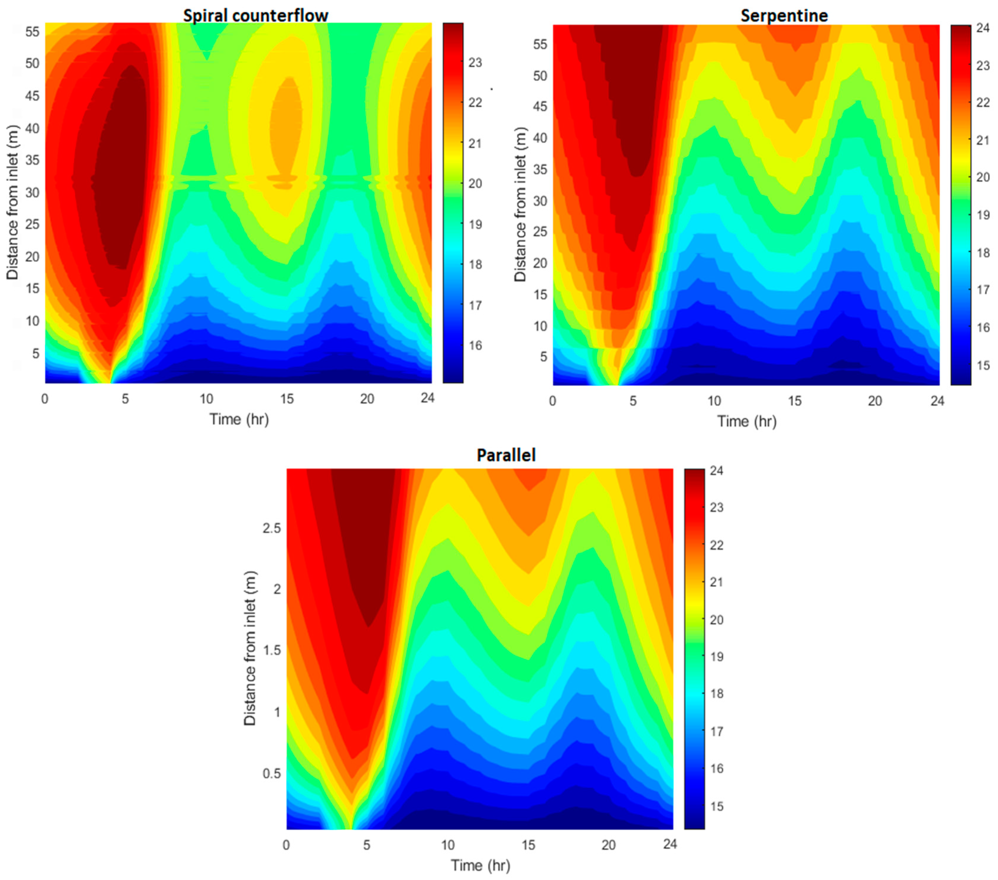
Figure 12 illustrates the wall surface temperature contours for all configurations throughout the day. As depicted in Figure 12, the spiral configuration had a more evenly distributed temperature, with a maximum difference of 4 °C across the wall when compared to the serpentine and parallel configurations, which had maximum temperature differences of 6.5 °C and 6.7 °C, respectively. The variation in temperature uniformity between configurations is caused by the arrangement of pipes in the wall. In a spiral configuration, the cool supply water and less cool return water are parallel and therefore provide a more uniform cooling flux density to the wall. This difference in pipe layout also affects the minimum wall surface temperature, which is crucial for determining the permissible indoor RH.

Table 3. Allowable indoor RH and temperature uniformity indicator for all configurations (S = 5 cm).

Configuration	${\mathit{T}}_{{\mathit{w}\mathit{a}\mathit{l}\mathit{l}}_{\mathit{m}\mathit{i}\mathit{n}}}$$/{\mathit{T}}_{\mathit{a}\mathit{i}\mathit{r}}$ (°C)	Allowable RH (%)	${\mathbf{\Delta }\mathit{T}}_{\mathit{u}}$ (°C)
spiral	15/25	≤53.8	4.0
	16.5/30	≤44.2	4.5
serpentine	14.5/25	≤52.1	6.5
	15.6/30	≤41.7	6.9
parallel	14.37/25	≤51.7	6.7
	15.25/30	≤40.8	7.0

provides a guide to determining the allowable indoor RH to minimize the risk of condensation on the wall surface based on all temperature scenarios for the three piping configurations. Furthermore, Table 3 displays the cases, along with the corresponding difference between the maximum and minimum wall surface temperature (${\mathrm{\Delta }T}_u$). This difference serves as an indicator of temperature uniformity.

For zone temperatures between 25 °C and 30 °C, the spiral configuration permits a higher indoor humidity level compared to the other configurations. The serpentine configuration allows for a 1% higher humidity level than the parallel configuration.

3.5.3. Cooling Heat Flux Density

Figure 13 shows the variation in cooling capacity in all modeled configurations for 24 h. As shown in Figure 13, the maximum cooling capacity was observed approximately two hours after the water flow rate reached its peak. Among the different configurations, the serpentine configuration exhibited the highest cooling capacity for a pipe spacing of $M$ = 10 cm, followed by the parallel and spiral configurations. Additionally, the difference in cooling capacity between the two spacings (i.e., the maximum distance between the two curves in Figure 13) was greater for the parallel configuration than for the other two configurations. Similar to $M$ = 10 cm, the serpentine configuration delivered the highest cooling capacity for $M$ = 30 cm, followed by the spiral and parallel configurations.

Table 4. Maximum cooling capacity (W/m²) for all scenarios.

Temperature Scenarios	Serpentine				Parallel				Spiral
	$\mathit{S}$ = 5 *		$\mathit{S}$ = 10		$\mathit{S}$ = 5		$\mathit{S}$ = 10		$\mathit{S}$ = 5		$\mathit{S}$ = 10
	$\mathit{M}$ = 10 **	$\mathit{M}$ = 30	$\mathit{M}$ = 10	$\mathit{M}$ = 30	$\mathit{M}$ = 10	$\mathit{M}$ = 30	$\mathit{M}$ = 10	$\mathit{M}$ = 30	$\mathit{M}$ = 10	$\mathit{M}$ = 30	$\mathit{M}$ = 10	$\mathit{M}$ = 30
$T_{SW}$ = 12 °C	54.0	36.0	46.1	33.9	53.8	31.9	45.8	30.0	50.0	35.0	41.2	32.6
$T_{air}$ = 25 °C
$T_{SW}$ = 12 °C	80.0	53.5	68.0	49.7	79.1	46.8	67.6	44.4	73.9	51.9	60.8	48.0
$T_{air}$ = 30 °C
$T_{SW}$ = 15 °C	40.5	27.0	34.5	25.2	40.2	24.9	34.3	22.7	37.5	26.4	31.0	24.4
$T_{air}$ = 25 °C
$T_{SW}$ = 15 °C	65.0	43.9	55.8	40.8	64.8	38.5	55.4	36.5	60.8	42.7	49.9	39.3
$T_{air}$ = 30 °C

* Wall thickness in cm. ** Pipe spacing in cm.

presents the maximum cooling capacity for all scenarios simulated in this study.

Based on Table 4, the greatest decrease in maximum cooling capacity occurred at S = 5 cm when the pipe spacing was changed from 10 cm to 30 cm. As a result of increased spacing, the cooling capacity for the serpentine configuration decreased by 33% for S = 5 cm and 27% for S = 10 cm. Moreover, when the pipe spacing was increased from 10 cm to 30 cm, the cooling capacity decreased by 40% and 34% for the parallel configuration at S = 5 cm and S = 10 cm, respectively. Similarly, for the spiral configuration, the decreases were 30% and 21%. These results suggest that pipe spacing has a more significant impact on maximum cooling capacity than wall thickness does.

To better understand the DCW-wall system performance in the context of existing water-based cooling systems,

Table 5. Maximum cooling capacity of various water-based cooling systems.

Study	Cooling Capacity (W/m2)	$\mathit{S}$ (cm) *	${\mathit{T}}_{\mathit{S}\mathit{W}}$ (°C) **	${\mathit{T}}_{\mathit{a}\mathit{i}\mathit{r}}$ (°C)	Description
[57]	56 for $S$ = 10 cm	2.5 & 10	5	23.3	Hydronic pipe embedded wall system with active insulation system and thermal energy storage
	82 for $S$ = 2.5 cm
[58]	16 for $T_{SW}$ = 15 °C	15	15 & 20	26	Chilled water in pipes embedded in the wall core. Wall has a 5 cm of insulation.
	29 for $T_{SW}$ = 20 °C
[25]	10–21	10	20	26	Pipes attached to insulating brick
[26]	35–40	15	18	26	Pipes in the plaster layer
[59]	66.3 for $T_{SW}$ = 12 °C	15	12 & 15	26 & 26.4	The wall is made of plaster board, pipe attached to an aluminum foil, and a 5 cm insulation layer.
	50.2 for $T_{SW}$ = 15 °C
Current	54–80 for $T_{SW}$ = 12 °C	10 & 30	12 & 15	25 & 30	DCW-wall system
	41–65 for $T_{SW}$ = 15 °C

* Pipe spacing ** Water supply temperature.

provides details on the maximum cooling capacity and associated parameters of the DCW-wall system and recent water-based cooling systems.

3.5.4. Delivered Cooling Energy

Figure 14 shows the changes in the cumulative total DCE, DCE to room, and energy stored in the wall over a 24-h period for all configurations. The cumulative DCE trends depicted in Figure 14 exhibit similar behavior for all configurations and are discussed in Section 3.4. In this context, although thermal mass did not significantly contribute to heat/cold storage, it could stabilize the wall surface temperature and cooling capacity throughout the day.

Table 6. Total DCE (MJ) per day for all scenarios.

Temperature Scenarios	Serpentine				Parallel				Spiral
	$\mathit{S}$ = 5		$\mathit{S}$ = 10		$\mathit{S}$ = 5		$\mathit{S}$ = 10		$\mathit{S}$ = 5		$\mathit{S}$ = 10
	$\mathit{M}$ = 10	$\mathit{M}$ = 30	$\mathit{M}$ = 10	$\mathit{M}$ = 30	$\mathit{M}$ = 10	$\mathit{M}$ = 30	$\mathit{M}$ = 10	$\mathit{M}$ = 30	$\mathit{M}$ = 10	$\mathit{M}$ = 30	$\mathit{M}$ = 10	$\mathit{M}$ = 30
$T_{SW}$ = 12 °C	21.92	16.11	20.90	15.97	21.80	15.13	19.90	14.61	20.0	15.17	19.0	15.0
$T_{air}$ = 25 °C
$T_{SW}$ = 12 °C	29.97	23.10	28.80	21.82	29.20	20.44	28.3	20.11	26.3	22.32	26.0	22.0
$T_{air}$ = 30 °C
$T_{SW}$ = 15 °C	16.93	13.0	16.2	12.4	15.2	10.8	15.0	10.3	16.0	12.4	14.1	12.2
$T_{air}$ = 25 °C
$T_{SW}$ = 15 °C	25.31	17.91	24.0	17.7	24.0	16.42	23.10	15.8	23.0	18.32	22.0	18.0
$T_{air}$ = 30 °C

presents the total DCE values for all scenarios. Similar to cooling capacity, the serpentine configuration showed the highest cooling energy delivered by the system in all temperature scenarios.

3.6. Influence of Wall Surface Area on Total DCE

In addition to the previously mentioned influential parameters, changes in wall dimensions affect the total DCE due to the change in pipe length and, therefore, the area of heat transfer. For the temperature scenario of $T_{SW}$ = 12 °C and $T_{air}$ = 25 °C with a wall thickness of 5 cm,

Table 7. Total DCE (MJ) per day for different wall surface areas.

Configuration	Wall Surface Area (m2)
	4		6		8		10		12
	$\mathit{M}$ = 10	$\mathit{M}$ = 30	$\mathit{M}$ = 10	$\mathit{M}$ = 30	$\mathit{M}$ = 10	$\mathit{M}$ = 30	$\mathit{M}$ = 10	$\mathit{M}$ = 30	$\mathit{M}$ = 10	$\mathit{M}$ = 30
spiral	16.11	12.21	20	15.17	22.0	18.13	23.94	20.10	25.0	22.0
serpentine	18.04	12.0	21.92	16.11	25.07	18.0	27.20	20.0	28.10	21.90
parallel	17.0	11.24	21.80	15.13	23.90	17.10	26.0	18.90	28.0	20.80

shows the simulation results of the total DCE for all configurations with respect to changes in wall surface area (wall height was fixed at 2 m, but length was subject to change).

As shown in Table 7, on average, expanding the wall surface area from 4 m² to 6 m² resulted in a 21% increase in total DCE for pipe spacing of $M$ = 10 cm and a 29% increase for $M$ = 30 cm. Furthermore, for $M$ = 10 cm, when the wall surface area was increased in a 2 m² increment, from 6 m² to 8 m², 8 m² to 10 m², and 10 m² to 12 m², the total DCE increased by 10%, 7.2%, and 4.4%, respectively, with a diminishing gain. For $M$ = 30 cm, the values are 11.1%, 10%, and 8.9%, respectively. Table 7 reveals that while both an increase in wall surface area and a decrease in pipe spacing lead to an increase in total DCE, the impact of the latter is more pronounced.

4. Conclusions

This study aimed to assess the cooling potential of a DCW-wall system and establish guidelines to prevent condensation on the wall surface. A 3D transient thermal model was utilized and validated with experimental data from a similar study. The model incorporated a typical DCW flow rate pattern to calculate various parameters under different operational and boundary conditions. The results indicated that smaller pipe spacing, lower water inlet temperature, and thinner walls led to increased cooling capacity and total DCE. The serpentine configuration exhibited the highest cooling potential, with a maximum cooling capacity of 80.0 W/m² and a total DCE of 29.97 MJ/day. The free cooling energy provided by the DCW-wall system can effectively reduce or even eliminate reliance on mechanical cooling systems during cooling seasons in cold-climate residential buildings without wasting DCW resources. The findings revealed that the DCW-wall system with spiral configuration supplied almost 11% of the energy demand for space cooling during the cooling season in Toronto, Canada. In addition, the three configurations demonstrated the lowest average wall surface temperature, ranging from 18.6 °C to 21.2 °C across all operation and boundary scenarios. The 10 cm-thick wall had a surface temperature 1 °C higher than the 5 cm-thick wall at peak cooling capacity. The spiral counterflow configuration maintained the most uniform temperature on the wall surface, which is crucial for thermal comfort and condensation prevention. As a result, a conservative, yet simple, guideline was proposed to prevent condensation. Maintaining indoor RH levels between 40.8% and 53.8% would minimize the likelihood of condensation, regardless of the operation and boundary scenario.

This study has certain limitations that are worth considering. First, the research is limited to simulation and validation using experimental data from another similar system. While this approach provides accurate and valuable insights, conducting an experimental study that matches the proposed DCW-wall system configurations will provide more assuring validation. If experimental validation is not possible, using other commercial simulation software to verify the results obtained from the 3D model would be beneficial. Addressing these limitations will enhance the accuracy, applicability, and robustness of the research findings. Additionally, future work could consider incorporating outdoor environmental factors, such as temperature and RH, to account for their impact on indoor conditions. Conducting experimental studies with varied engineering designs, employing additional simulation software for verification, and exploring the influence of outdoor variables on indoor climate should be the focus of future studies.

References

1. Dodoo, A.; Gustavsson, L.; Sathre, R. Building energy-efficiency standards in a life cycle primary energy perspective. Energy Build. 2011, 43, 1589–1597. [Google Scholar] [CrossRef]
2. Edenhofer, O.; Pichs-Madruga, R.; Sokona, Y.; Farahani, E.; Kadner, S.; Eickemeier, P. Intergovernmental Panel on Climate Change (IPCC): Mitigation of Climate Change. In Contribution of Working Group III to the Fifth Assessment Report of the Intergovernmental Panel on Climate Change; Cambridge University Press: Cambridge, UK, 2014. [Google Scholar]
3. Andreou, A.; Barrett, J.; Taylor, P.G.; Brockway, P.E.; Wadud, Z. Decomposing the drivers of residential space cooling energy consumption in EU-28 countries using a panel data approach. Energy Built Environ. 2020, 1, 432–442. [Google Scholar] [CrossRef]
4. Dutta, S.; Hussain, C.M. Sustainable Fuel Technologies Handbook; Academic Press: New York, NY, USA, 2020. [Google Scholar]
5. Mugnini, A.; Polonara, F.; Arteconi, A. Energy flexibility curves to characterize the residential space cooling sector: The role of cooling technology and emission system. Energy Build. 2021, 253, 111335. [Google Scholar] [CrossRef]
6. Santamouris, M.; Kolokotsa, D. Passive cooling dissipation techniques for buildings and other structures: The state of the art. Energy Build. 2013, 57, 74–94. [Google Scholar] [CrossRef]
7. Bulut, H.; Aktacir, M.A. Determination of free cooling potential: A case study for Istanbul, Turkey. Appl. Energy 2011, 88, 680–689. [Google Scholar] [CrossRef]
8. International Energy Agency (IEA). Ventilative Cooling. In Status and Recommendations for Better Implementation of Ventilative Cooling in Standards, Legislation and Compliance Tools (Background Report); International Energy Agency (IEA): Paris, France, 2018. [Google Scholar]
9. Katili, A.R.; Boukhanouf, R.; Wilson, R. Space cooling in buildings in hot and humid climates—A review of the effect of humidity on the applicability of existing cooling techniques. In Proceedings of the 14th International Conference on Sustainable Energy Technologies, Nottingham, UK, 25–27 August 2015. [Google Scholar]
10. Guo, X.; Hendel, M. Urban water networks as an alternative source for district heating and emergency heat-wave cooling. Energy 2018, 145, 79–87. [Google Scholar] [CrossRef] [Green Version]
11. van der Hoek, J.P.; Mol, S.; Giorgi, S.; Ahmad, J.I.; Liu, G.; Medema, G. Energy recovery from the water cycle: Thermal energy from drinking water. Energy 2018, 162, 977–987. [Google Scholar] [CrossRef]
12. Ahmad, J.I.; Giorgi, S.; Zlatanovic, L.; Liu, G.; van der Hoek, J.P. Maximizing Thermal Energy Recovery from Drinking Water for Cooling Purpose. Energies 2021, 14, 2413. [Google Scholar] [CrossRef]
13. Prybysh, R.; Al-Hussein, M.; Fleck, B.; Sadrzadeh, M.; Osolu, J. Experimental Study on the Palatability Impacts of Potable Water as a Hydronic Medium. Water 2018, 10, 218. [Google Scholar] [CrossRef] [Green Version]
14. Babiak, J.; Vagiannis, G. Thermally Activated Building System (TABS): Efficient Cooling and Heating of Commercial Buildings. In Proceedings of the CLIMAMED 2015, Juan les Pins, France, 10–11 September 2015. [Google Scholar]
15. Ma, P.; Wang, L.-S.; Guo, N. Energy storage and heat extraction–From thermally activated building systems (TABS) to thermally homeostatic buildings. Renew. Sustain. Energy Rev. 2015, 45, 677–685. [Google Scholar] [CrossRef]
16. Romaní, J.; de Gracia, A.; Cabeza, L.F. Simulation and control of thermally activated building systems (TABS). Energy Build. 2016, 127, 22–42. [Google Scholar] [CrossRef] [Green Version]
17. Chung, W.J.; Park, S.H.; Yeo, M.S.; Kim, K.W. Control of Thermally Activated Building System Considering Zone Load Characteristics. Sustainability 2017, 9, 586. [Google Scholar] [CrossRef] [Green Version]
18. Guerrero, M.; Sánchez, J.; Álvarez, S.; Tenorio, J.A.; Cabeza, L.F.; Bartolomé, C.; Pavón, M. Evaluation of the Behavior of an Innovative Thermally Activated Building System (TABS) with PCM for an Efficient Design. In Proceedings of the CLIMA 2019 Congress, Bucharest, Romania, 26–29 May 2019; EDP Sciences: Les Ulis, France, 2019. [Google Scholar]
19. Krajčík, M.; Arıcı, M.; Šikula, O.; Šimko, M. Review of water-based wall systems: Heating, cooling, and thermal barriers. Energy Build. 2021, 253, 111476. [Google Scholar] [CrossRef]
20. Antonopoulos, K.; Vrachopoulos, M.; Tzivanidis, C. Experimental and theoretical studies of space cooling using ceiling-embedded piping. Appl. Therm. Eng. 1997, 17, 351–367. [Google Scholar] [CrossRef]
21. Xie, J.-L.; Zhu, Q.-Y.; Xu, X.-H. An active pipe-embedded building envelope for utilizing low-grade energy sources. J. Cent. South Univ. 2012, 19, 1663–1667. [Google Scholar] [CrossRef]
22. Shin, M.S.; Rhee, K.N.; Ryu, S.R.; Yeo, M.S.; Kim, K.W. Design of radiant floor heating panel in view of floor surface temperatures. Build. Environ. 2015, 92, 559–577. [Google Scholar] [CrossRef]
23. Romaní, J.; Cabeza, L.F.; de Gracia, A. Development and experimental validation of a transient 2D numeric model for radiant walls. Renew. Energy 2018, 115, 859–870. [Google Scholar] [CrossRef] [Green Version]
24. Šimko, M.; Petráš, D.; Krajčík, M.; Szabó, D. Testing of a Radiant Wall Cooling System with Pipes Coupled to Aerated Blocks. Period. Polytech. Mech. Eng. 2022, 66, 59–66. [Google Scholar] [CrossRef]
25. Krajčík, M.; Šikula, O. The possibilities and limitations of using radiant wall cooling in new and retrofitted existing buildings. Appl. Therm. Eng. 2020, 164, 114490. [Google Scholar] [CrossRef]
26. Krajčík, M.; Šimko, M.; Šikula, O.; Szabó, D.; Petráš, D. Thermal performance of a radiant wall heating and cooling system with pipes attached to thermally insulating bricks. Energy Build. 2021, 246, 111122. [Google Scholar] [CrossRef]
27. Šimko, M.; Krajčík, M.; Šikula, O. Radiant Wall Cooling with Pipes Arranged in Insulation Panels Attached to Facades of Existing Buildings. In Proceedings of the CLIMA 2019 Congress, Bucharest, Romania, 26–29 May 2019; EDP Sciences: Les Ulis, France, 2019. [Google Scholar]
28. Samuel, D.L.; Nagendra, S.S.; Maiya, M.P. Parametric analysis on the thermal comfort of a cooling tower based thermally activated building system in tropical climate—An experimental study. Appl. Therm. Eng. 2018, 138, 325–335. [Google Scholar] [CrossRef]
29. Junasová, B.; Krajčík, M.; Šikula, O.; Arıcı, M.; Šimko, M. Adapting the construction of radiant heating and cooling systems for building retrofit. Energy Build. 2022, 268, 112228. [Google Scholar] [CrossRef]
30. Babiak, J.; Olesen, B.W.; Petras, D. Low Temperature Heating and High Temperature Cooling: Rehva Guidebook No 7; REHVA: Ixelles, Belgium, 2007. [Google Scholar]
31. Behrendt, B. Possibilities and Limitations of Thermally Activated Building Systems: Simply TABS and a Climate Classification for TABS; Technical University of Denmark: Lyngby, Denmark, 2016. [Google Scholar]
32. Lehmann, B.; Dorer, V.; Gwerder, M.; Renggli, F.; Tödtli, J. Thermally activated building systems (TABS): Energy efficiency as a function of control strategy, hydronic circuit topology and (cold) generation system. Appl. Energy 2011, 88, 180–191. [Google Scholar] [CrossRef]
33. ASHRAE. 2016 ASHRAE Handbook-HVAC Systems and Equipment (IP Edition); ASHRAE: Peachtree Corners, GA, USA, 2016. [Google Scholar]
34. Kappel, K.; Grechenig, T. “show-me” water consumption at a glance to promote water conservation in the shower. In Proceedings of the 4th International Conference on Persuasive Technology, Claremont, CA, USA, 26–29 April 2009. [Google Scholar]
35. Beal, C.D.; Stewart, R.A. Identifying residential water end uses underpinning peak day and peak hour demand. J. Water Resour. Plan. Manag. 2014, 140, 04014008. [Google Scholar] [CrossRef] [Green Version]
36. Cole, G.; Stewart, R.A. Smart meter enabled disaggregation of urban peak water demand: Precursor to effective urban water planning. Urban Water J. 2013, 10, 174–194. [Google Scholar] [CrossRef] [Green Version]
37. Legget, R.; Peckover, F. Soil Temperature Studies—A Progress Report. 1949. Available online: https://onlinepubs.trb.org/Onlinepubs/hrbproceedings/29/29-030.pdf (accessed on 20 April 2023).
38. Tham, S.; Thompson, R.; Landeg, O.; Murray, K.; Waite, T. Indoor temperature and health: A global systematic review. Public Health 2020, 179, 9–17. [Google Scholar] [CrossRef]
39. Oetomo, A.; Jalali, N.; Costa, P.D.P.; Morita, P.P. Indoor temperatures in the 2018 heat wave in Quebec, Canada: Exploratory study using Ecobee smart thermostats. JMIR Form. Res. 2022, 6, e34104. [Google Scholar] [CrossRef]
40. Patankar, S.V. Numerical Heat Transfer and Fluid Flow; CRC Press: Boca Raton, FL, USA, 2018. [Google Scholar]
41. Merabtine, A.; Mokraoui, S.; Kheiri, A.; Dars, A.; Hawila, A.A.W. Fundamentals of Heat and Mass Transfer; John Wiley & Sons: Hoboken, NJ, USA, 2011. [Google Scholar]
42. Baldinelli, G.; Bianchi, F.; Rotili, A.; Presciutti, A. Transient heat transfer in radiant floors: A comparative analysis between the lumped capacitance method and infrared thermography measurements. J. Imaging 2016, 2, 22. [Google Scholar] [CrossRef] [Green Version]
43. Merabtine, A.; Mokraoui, S.; Kheiri, A.; Dars, A.; Hawila, A.A.W. Experimental and multidimensional numerical analysis of the thermal behavior of an anhydrite radiant slab floor heating system: A multi-objective sensitivity study. Energy Build. 2018, 174, 619–634. [Google Scholar] [CrossRef]
44. Femp, M. Guidelines: Measurement and Verification for Federal Energy Projects, Version 3.0. In Energy Efficiency and Renewable Energy; United States Department of Energy: Washington, DC, USA, 2008. [Google Scholar]
45. Xing, D.; Li, N.; Zhang, C.; Heiselberg, P. A critical review of passive condensation prevention for radiant cooling. Build. Environ. 2021, 205, 108230. [Google Scholar] [CrossRef]
46. Xie, D.; Wang, Y.; Wang, H.; Mo, S.; Liao, M. Numerical analysis of temperature non-uniformity and cooling capacity for capillary ceiling radiant cooling panel. Renew. Energy 2016, 87, 1154–1161. [Google Scholar] [CrossRef]
47. Ning, B.; Chen, Y.; Liu, H.; Zhang, S. Cooling capacity improvement for a radiant ceiling panel with uniform surface temperature distribution. Build. Environ. 2016, 102, 64–72. [Google Scholar] [CrossRef]
48. United States Environmental Protection Agency; Office of Air and Radiation, Indoor Environments Division. Mold Remediation in Schools and Commercial Buildings; ERIC Clearinghouse, United States Department of Education: Washington, DC, USA, 2001. [Google Scholar]
49. Cholewa, T.; Rosiński, M.; Spik, Z.; Dudzińska, M.R.; Siuta-Olcha, A. On the heat transfer coefficients between heated/cooled radiant floor and room. Energy Build. 2013, 66, 599–606. [Google Scholar] [CrossRef]
50. Cholewa, T.; Anasiewicz, R.; Siuta-Olcha, A.; Skwarczynski, M.A. On the heat transfer coefficients between heated/cooled radiant ceiling and room. Appl. Therm. Eng. 2017, 117, 76–84. [Google Scholar] [CrossRef]
51. Government of Canada. Weather, Climate, and Hazard—Historical Data. 2021. Available online: https://climate.weather.gc.ca/historical_data/search_historic_data_e.html (accessed on 15 August 2022).
52. WeatherStats. Toronto Historical Relative Humidity. 2022. Available online: https://toronto.weatherstats.ca/metrics/relative_humidity.html (accessed on 18 May 2022).
53. Natural Resources Canada. Energy Fact Book 2019–2020; Natural Resources Canada Ottawa: Ottawa, ON, Canada, 2019. [Google Scholar]
54. Statistics Canada. Household Energy Consumption, Canada and Provinces. 2019. Available online: https://www150.statcan.gc.ca/t1/tbl1/en/tv.action?pid=2510006001 (accessed on 15 August 2022).
55. Purushothama, B. Humidification and Ventilation Management in Textile Industry; CRC Press: Boca Raton, FL, USA, 2010. [Google Scholar]
56. Government of Canada. Air Conditioning Your Home. 2016. Available online: https://www.nrcan.gc.ca/energy-efficiency/energy-star-canada/about/energy-star-announcements/publications/air-conditioning-your-home/6051 (accessed on 1 February 2023).
57. Iffa, E.; Hun, D.; Salonvaara, M.; Shrestha, S.; Lapsa, M. Performance evaluation of a dynamic wall integrated with active insulation and thermal energy storage systems. J. Energy Storage 2022, 46, 103815. [Google Scholar] [CrossRef]
58. Krajčík, M.; Šikula, O. Heat storage efficiency and effective thermal output: Indicators of thermal response and output of radiant heating and cooling systems. Energy Build. 2020, 229, 110524. [Google Scholar] [CrossRef]
59. Koca, A.; Karakoyun, Y.; Acikgoz, O.; Dogu, M.; Dalkilic, A.S. An experimental investigation on the radiant cooled wall’s heat transfer characteristics in a fully conditioned real-sized living environment. Energy Build. 2022, 277, 112578. [Google Scholar] [CrossRef]
Figure 1. DCW-wall system.
Buildings 13 01491 g001
Figure 2. Piping patterns.
Buildings 13 01491 g002
Figure 3. Daily pattern of average hourly water consumption for residential buildings.
Buildings 13 01491 g003
Figure 4. Schematic of the wall and thermal transmittances between a water node and its adjacent wall node.
Buildings 13 01491 g004
Figure 5. Measured and simulated average floor surface temperatures.
Buildings 13 01491 g005
Figure 6. Average wall surface temperature over the 24-h period ( T S W = 12 °C, T a i r = 25 °C, S = 5 cm).
Buildings 13 01491 g006
Figure 7. Water outlet temperature over the 24-h period ( T S W = 12 °C, T a i r = 25 °C, S = 5 cm).
Buildings 13 01491 g007
Figure 8. Wall surface temperature versus the distance from the inlet over the 24-h period ( T S W = 12 °C, T a i r = 25 °C, S = 5 cm).
Buildings 13 01491 g008
Figure 9. Cooling capacity over the 24-h period ( T S W = 12 °C, T a i r = 25 °C, S = 5 cm).
Buildings 13 01491 g009
Figure 10. Cumulative DCE over the 24-h period ( T S W = 12 °C, T a i r = 25 °C, S = 5 cm).
Buildings 13 01491 g010
Figure 11. Average wall surface temperature for all configurations over a period of 24 h ( T S W = 12 °C, T a i r = 25 °C, S = 5 cm).
Buildings 13 01491 g011
Figure 12. Wall surface temperature versus the distance from the inlet for all configurations over the 24-h period ( T S W = 12 °C, T a i r = 25 °C, S = 5 cm).
Buildings 13 01491 g012
Figure 13. Cooling capacity for all configurations during the 24-h period ( T S W = 12 °C, T a i r = 25 °C, S = 5 cm).
Buildings 13 01491 g013
Figure 14. Cumulative DCE for all configurations over the 24-h period ( T S W = 12 °C, T a i r = 25 °C, S = 5 cm).
Buildings 13 01491 g014