Article

Building Detection in High-Resolution Remote Sensing Images by Enhancing Superpixel Segmentation and Classification Using Deep Learning Approaches

by
Ayoub Benchabana
1,2,*,
Mohamed-Khireddine Kholladi
1,3,
Ramla Bensaci
4 and
Belal Khaldi
4
1
Department of Computer Science, University of El Oued, El Oued 39000, Algeria
2
Laboratory of Operator Theory and EDP: Foundations and Application, University of El Oued, El Oued 39000, Algeria
3
MISC Laboratory of Constantine 2, University of Constantine 2, El Khroub 25016, Algeria
4
Laboratory of Artificial Intelligence and Data Science, University of Kasdi Merbah Ouargla, PB. 511., Ouargla 30000, Algeria
*
Author to whom correspondence should be addressed.
Buildings 2023, 13(7), 1649; https://doi.org/10.3390/buildings13071649
Submission received: 13 June 2023 / Revised: 26 June 2023 / Accepted: 27 June 2023 / Published: 28 June 2023
(This article belongs to the Section Construction Management, and Computers & Digitization)

Abstract

:
Accurate building detection is a critical task in urban development and digital city mapping. However, current building detection models for high-resolution remote sensing images are still facing challenges due to complex object characteristics and similarities in appearance. To address this issue, this paper proposes a novel algorithm for building detection based on in-depth feature extraction and classification of adaptive superpixel shredding. The proposed approach consists of four main steps: image segmentation into homogeneous superpixels using a modified Simple Linear Iterative Clustering (SLIC), in-depth feature extraction using an variational auto-encoder (VAE) scale on the superpixels for training and testing data collection, identification of four classes (buildings, roads, trees, and shadows) using extracted feature data as input to an Convolutional Neural Network (CNN), and extraction of building shapes through regional growth and morphological operations. The proposed approach offers more stability in identifying buildings with unclear boundaries, eliminating the requirement for extensive prior segmentation. It has been tested on two datasets of high-resolution aerial images from the New Zealand region, demonstrating superior accuracy compared to previous works with an average F1 score of 98.83%. The proposed approach shows potential for fast and accurate urban monitoring and city planning, particularly in urban areas.

1. Introduction

The ongoing rapid urbanization and rural development have dramatically transformed our surroundings. Buildings are now the most visible and dominant features in urban regions. Consequently, identifying and recognizing building landmarks has become a crucial and complex task in various applications [1,2,3,4,5,6]. Fortunately, the advancement in technology has enabled the acquisition of high-resolution spatial images from aerial and satellite imagery, offering accurate technical details and rich textural features of land covers. The improved spatial resolution enhances the ability to distinguish between different urban objects, making it possible to extract more information about distinct building features [3,7,8,9]. Researchers have proposed numerous solutions to address this issue, which can be broadly categorized into physical rule-based approaches, image segmentation-based methods, and more recently, conventional machine learning and enhanced deep learning methods [10].
Building detection models for high-resolution remote sensing images can be classified into two categories: based on hand-crafted features or based on feature learning [11]. The first category primarily relies on creating detection models based on matching templates, SVMs, or ensemble of classifiers of spectral or textural building features. On the other hand, deep learning algorithms are typically used in the second category. In recent years, deep learning [12,13] has become a crucial technique for remote sensing, and has been extensively used in various remote sensing applications, including image processing. This study in [14] analyzes the approaches and trends in the field of deep learning for remote sensing, highlighting its potential and its wide application range.
Detecting buildings from aerial and satellite imagery is a daunting task due to the massive amount of pixel points that need to be processed, often making it challenging to handle large datasets in a fast and effective manner, even with modern computing frameworks. To address this challenge, researchers have proposed superpixel segmentation algorithms that group pixels to create contextually significant regions, leading to better processing efficiency while preserving important information [15]. Additionally, the homogeneity of these superpixels plays a crucial role in accurately detecting objects. The more homogeneous they are, the more accurate the detection will be.
To address the challenge of detecting buildings in aerial and satellite images, we have developed a new framework that involves the use of a variational auto-encoder (VAE) and convolutional neural networks (CNNs). Firstly, we reduce the resolution of the aerial image by converting it into a superpixel map. Next, we utilize VAE to model these superpixels efficiently and consistently and extract features from them. We then employ CNN as a classifier to obtain a final decision regarding each superpixel. Finally, we apply regional growth, morphological operations, and a contouring process to determine the final shape of the buildings. The present framework makes a threefold contribution: (1) a new structure for building detection from high-resolution images that improves the model’s capacity to recognize various building shapes; (2) an adaptive superpixel (SLIC) algorithm that generates more meaningful, consistent superpixels without excessive smoothness to preserve the boundaries of the edges; and (3) an enhanced regional growth approach to maintain and recognize the exacted building shapes.
The rest of the paper is structured as follows: Section 2 provides an overview of related work in the field of building detection. In Section 3, we delve into detailed explanations and illustrations of the proposed methods. Section 4 gives a detailed analysis of how the parameters were chosen, how the system was set up, and what the results of the experiments were. In Section 5, we conclude the paper and put forward some perspectives.

2. Related Work

Detecting buildings and other objects in remotely sensed images has garnered significant research interest in recent years [16,17,18,19,20,21,22], with many proposed strategies. In [23], the authors presented an adapted U-Net convolutional neural network segmentation to identify buildings using LiDAR data, based on the premise that U-Net performed well in detecting irregular edges. The study found that the model performed well for residential buildings but struggled with larger structures and had difficulty identifying diagonally oriented buildings, resulting in some buildings being merged or split. In [11], the authors introduced the Res2-Unet model, which employed multiscale learning to increase the size of each bottleneck layer’s responsive fields. They suggested using a boundary loss function to improve detection performance and generate accurate building boundaries. However, the model still struggled to differentiate certain roads from buildings, and sometimes it mistook background objects for buildings while entirely removing some buildings with spectral and textural properties similar to the background land. In [24], three parallel CNN stream channels have been used to detect buildings: high-resolution aerial imagery, the digital surface model (DSM), and deep feature extraction through merging previous channels. The final building shape was determined by morphological operations. Although this approach yields high accuracy in detecting small buildings, it is incapable of detecting gaps among buildings in densely populated or low-height regions.
Nevertheless, the traditional pixel-based deep learning approach (CNN) requires a lot of computational power and storage space. Therefore, superpixel-based classification has recently attracted much interest. Moreover, in [15], using OpenStreetMap as semantic tags, the CNN model is trained to classify superpixels generated by Simple Linear Iterative Clustering (SLIC). Their main problem was that some superpixels contained both building and non building pixels, leading to overlapping feature data and misclassifying results. Furthermore, Ref. [25] evaluates the compactness index value of four superpixel algorithms using the same appropriate settings based on previous tests. They find that both SLIC and SEED superpixel algorithms have low compactness values and prefer the second because of the well-aligned segment with object boundaries. In [26], the authors suggest the ConvCRF model as an integration of conditional random field CRF and CNN, combined with superpixel boundary constraint. They conducted analytical experiments compared to multiple commonly used machine-learning algorithms, including SVM and CNN. The deep models are proven to be less sensitive to similar object types with low backscattering intensity. In addition, Ref. [27] proposed a fused DeepLab v2 neural network classification result with the SLIC segment for boundary recognizing to assess earthquake-damaged buildings. Next, a mathematical morphological approach was included to reduce the background noise, except it causes the elimination of the fine lines of the boundaries.

3. Methodology

As shown in Figure 1, the overall framework of the proposed SP_VAE-CNN approach for building detection consists of four main steps: image segmentation using adaptive SLIC into patches, feature extraction from the segmented patches using VAE, classification of these features using CNN, and finally, a regional growth from the seeds point location followed with the morphological operation methods to determine the final shape of the buildings.

3.1. Superpixel Segmentation

Superpixel segmentation algorithms are proven to be efficient in computer vision. They have successfully been utilized to decrease the number of image primitives needed for further processing. Grouping similar pixels into homogeneous regions with perceptual meanings offers a compressed representation in the form of superpixels, which in turn greatly reduces the computation time. In particular, Simple Linear Iterative Clustering (SLIC) has demonstrated its effectiveness regarding object boundary adherence, speed, and minimal memory required [28]. It is a k-means-based local clustering of pixels into superpixels depending on their color similarity and nearness in the image. Typically, each pixel is represented by a five-dimensional [l, a, b, x, y] feature vector, where [l, a, b] are the channels of CIELAB color space and [x, y] are the pixel coordinates, from which the distance is measured. A superpixel’s components are primarily determined by color values, which provide limited information. Additionally, the superpixel’s size and compactness are controlled by the spatial proximity’s weighted distance controls, which may result in boundary distortion and losses due to their high values. To improve the feature representation and increase the significance of the superpixels, we use the integrative color intensity co-occurrence matrix (ICICM) [29] to compute the texture features and extend the feature vector into an eight-dimensional [l, a, b, e, h, c, x, y] where e, h, and c are, respectively, the energy, homogeneity, and correlation. The distance is defined by Equation (1).
D s = α D l a b + β D e h c + γ D x y
D l a b = l k l i 2 + a k a i 2 + b k b i 2
D e h c = e k e i 2 + h k h i 2 + c k c i 2
D x y = x k x i 2 + y k y i 2
where k and i are, respectively, the indices of the superpixels’ centers and their surrounding pixels, α, β and γ are the balance weight factor that controls the relativity of color similarity, texture and spatial proximity of superpixels, and S is the grid interval between them.
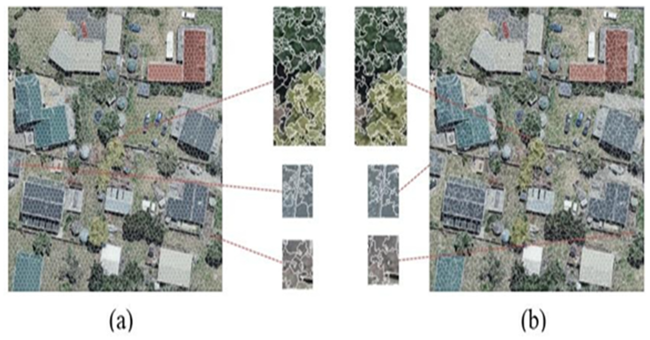
Figure 2 shows that incorporating texture features to the distance equation significantly improves the final segmentation result, especially in regions of trees, due to their rich texture nature. Although there were no remarkable changes in the building segments, there was compensation for bare soil and driveway parts. The segments were randomly shaped and had more variety of content.

3.2. Variational Autoencoders for Feature Extraction

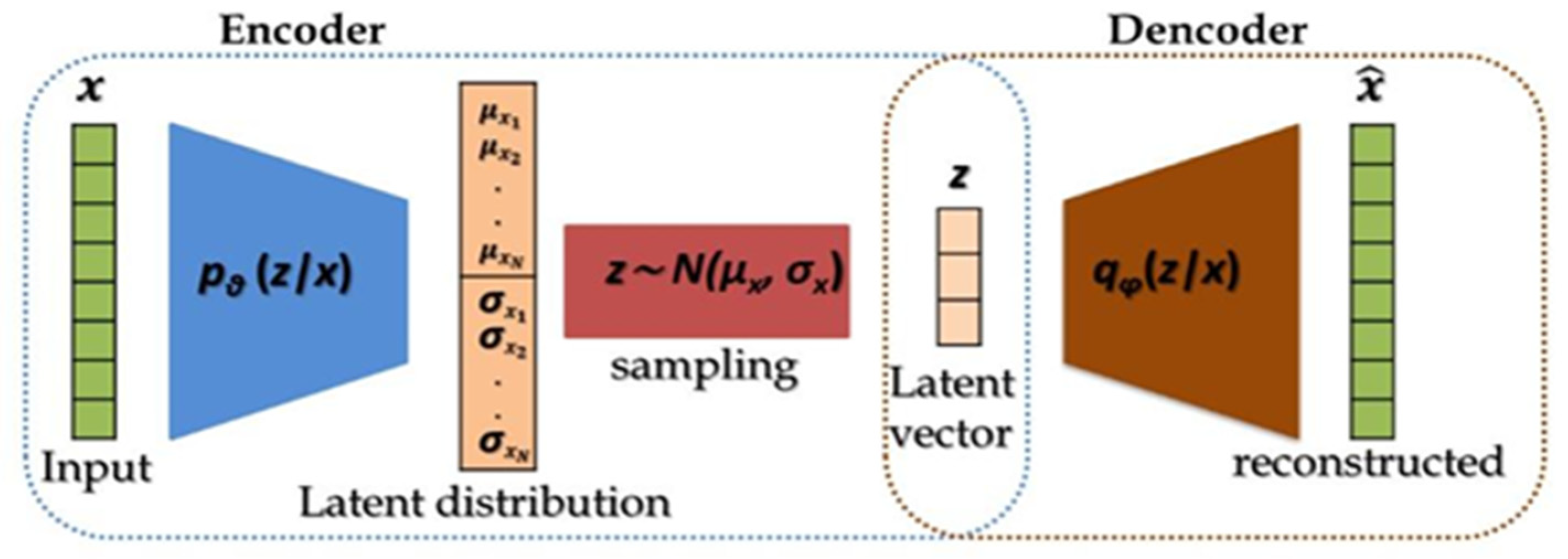
Autoencoders are unsupervised neural networks that learn effective representations of input data through an encoder and decoder. The encoder extracts features and creates a latent representation, which can be used for feature extraction on untrained data [30]. Variational Auto-Encoder by [31] is an advanced non-linear technique for feature extraction that can successfully and consistently describe data structure. The architecture of the autoencoder model is purposely constrained to a bottleneck at the model’s midline, from whence the input data rebuilding is conducted. VAE includes a variational constraint that the latent representation is a substance to a normal distribution, so the decoder’s output distribution corresponds to the observed data. The latent outputs are randomly selected from the distribution that the encoder has learned. The network structure of the VAE is presented in Figure 3.
x and x ^ denote the input and reconstructed input data, respectively. µ and σ denote the mean and variance of the gaussian distribution of the latent variable. z is a sample from N ( μ , σ 2 ) and h is the hidden layer in the network. The primary purpose of VAE is to train a network to reconstruct its input data x as x ^ using the following loss:
L x , x ^ = x x ^
Let us consider a dataset D = { x 1 , x 2 , , x N } of N independent and identically distributed variables, corresponding to the realizations of a random variable x X . We assume that the data are generated by some random process involving an unobserved continuous variable z generated from some prior normal distribution p θ = N ( μ , σ 2 ) .
The actual posterior density p θ z x is intractable. Therefore, we use a recognition model q φ z x , which is an approximation to the intractable true posterior p θ z x . We will minimize the K.L. divergence of the approximation from the true posterior. While K.L. divergence is zero, q φ z x is equal to p θ z x , that is p θ z x = q φ z x . The K.L. divergence of approximation from the true posterior D K L q φ z x p θ z x can be written as follows:
D K L q φ x p θ x = q φ x l o g l o g q φ x p θ x d z = l o g l o g p θ x + D K L q φ x p θ z E q φ x l o g l o g p θ z 0
That is:
l o g l o g p θ x D K L q φ x p θ z + E q φ x l o g l o g p θ z
The right half of the inequality is called the variational lower bound on the marginal likelihood of data x.
L θ , φ ; x = D K L q φ x p θ z + E q φ x l o g l o g p θ z
The first term D K L q φ z x p θ z of Equation (8) can be integrated analytically, and the second term E q φ z x l o g p θ x z requires estimation by sampling:
Firstly, we reparameterize the approximation q φ z x using a differentiable transformation (x, ε) of an auxiliary noise variable ε. Secondly, we estimate E q φ z x l o g p θ x z :
E q φ x l o g l o g p θ z = 1 M m = 1 M l o g l o g p θ z m
The parameters φ and θ of Equation (8) are estimated, in our case, using a fully connected neural network. Additionally, parameters can be updated using SGD, Adagrad [32], Adadelta [33], and Adam [34] optimizer.
After the training of the VAE is complete, only the encoder has been extracted and used for feature extraction from patches of the images.

3.3. Accurate Buildings Locations and Shapes

The first step is to determine the initial set of superpixel seed points. Depending on the direction of the shadow cast, the primary set is the set of superpixels located in the building class and has a neighbor from the shadow’s classes. Hence, we frequently add each neighbor to the seed set that is located in the building class and has similar features. Next, starting from the centers of the seed set, regional growth is applied to get the primary shape of the buildings. Finally, open morphological operations have been used to remove the noise and fill the gaps to detect the final shape of the buildings. The robustness of the proposed approach in satellite image segmentation against noise effects is a significant consideration. Therefore, the method leverages morphological operations, which play a crucial role in alleviating the impact of noise. The images undergo a sequence of mathematical morphology operations, specifically morphological opening and closing. These operations are defined by the following equations:
Morphological Opening: I ⊖ B = (I ⊖ B) ⊕ B
Morphological Closing: I ⊕ B = (I ⊕ B) ⊖ B
where I represents the input image, B denotes the structuring element, and ⊕ represents erosion and dilation operations, respectively.
By employing techniques such as dilation, erosion, opening, and closing, the approach effectively reduces noise while preserving essential spatial details. This integration of morphological operations enhances the method’s ability to distinguish between noise artifacts and meaningful image features, resulting in more accurate and reliable satellite image segmentation, even in the presence of noise. Robustness evaluations and experiments can be conducted to validate the approach’s performance under diverse noise conditions, ensuring its suitability for real-world satellite image analysis tasks (Algorithm 1).
Algorithm 1: Accurate Buildings Locations and Shapes
1.
Determine the initial set of superpixel seed points:
Identify the superpixels that belong to the building class and have neighbors from the shadow’s classes.
Add each neighboring superpixel that is located in the building class and has similar features to the seed set.
2.
Regional growth for primary shape estimation:
Starting from the centers of the seed set, perform a regional growth operation.
Expand the region by including neighboring superpixels that are similar in features and located in the building class.
Continue this process until the primary shape of the buildings is obtained.
3.
Refine the shape using open morphological operations:
Apply open morphological operations to remove noise and fill gaps in the primary shape.
Use these operations to detect the final shape of the buildings accurately.

4. Experiments and Results Analysis

This section is devoted to proving the proposed scheme’s efficiency across three subsections. In the first subsection, we examine the impact of altering the parameters’ values of our algorithm. The second one examines the performance of various deep learning algorithms on building detection. Finally, a comparison against some relevant works is conducted to demonstrate the superiority of our proposed algorithms.
The experiments in question were conducted using three datasets, each with its own unique features.
  • WHU aerial imagery 2016 dataset: originally built by the New Zealand Land Information Services. In our experiments, we have used the edited version of the dataset introduced by [35]. It includes aerial images of 187,000 buildings down-sampled to 0.3 m ground resolution and cropped into 8189 tiles of 512 × 512 pixels. The samples were divided into a training set of 130,500 buildings, a validation set of 14,500 buildings, and a test set of 42,000 buildings.
  • Land Information New Zealand urban aerial image dataset of Masterton: It has a ground resolution of 0.075 m, and it was cropped into patches of size 1024 × 1024 pixels. The datasets were chosen for their ability to cover a variety of land types, including different roof color patterns and building shapes. This made them well-suited for testing the effectiveness of the building detection model being proposed.
  • We collected high-resolution Google Earth images from different sites in Touggourt, Algeria. The images are chosen to represent different building characteristics, such as sizes and shapes.
The experiments were conducted on a computer having an Intel® Core i7 processor running at 2.00 GHz with n cores, 16 GB of RAM, and an NVIDIA GeForce GT 720 GPU card. The method has been implemented, and results have been analyzed using both Python and Matlab.

4.1. Parameters Selection

4.1.1. SLIC Parameter

The most critical parameter in the SLIC algorithm is the number of superpixels in the input image, which affects the superpixel’s size and may cause disturbances in the semantics of image parts. Small superpixels will contain insufficient features for semantic detection, and larger sizes may cover different types of objects. Thus, initializing a suitable number of superpixels depends on its smallest assumed size and the dimensions of the studied area images. To ensure that the smallest size contains sufficient information, we set it to 16 × 16.

4.1.2. VAE Parameter and Performance

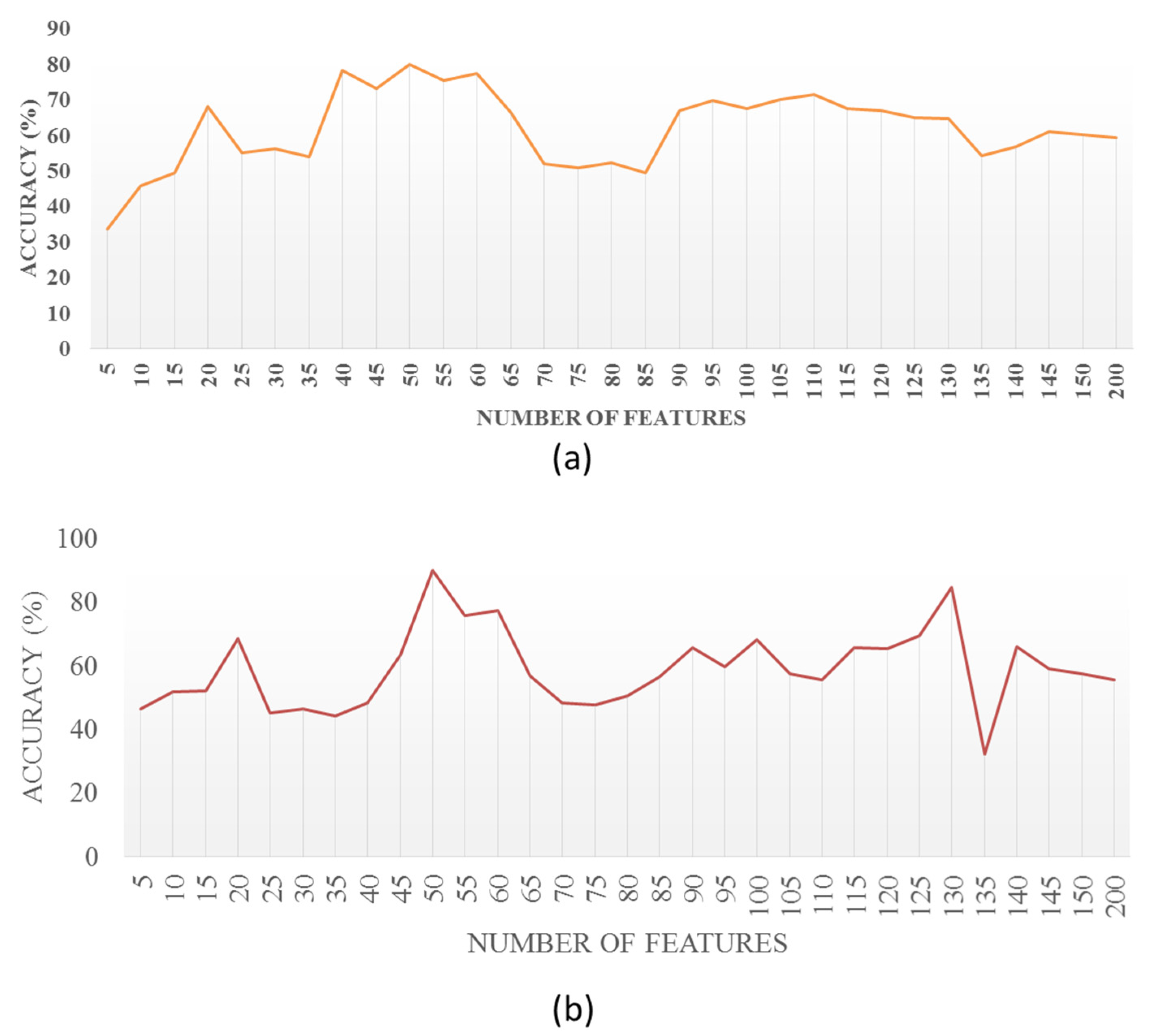
The VAE architecture used in our experiments consisted of four hidden layers, with two in the encoder and two in the decoder. The input size was determined based on the maximum size of the superpixels. The architecture had four hyperparameters, which included 128 nodes in the hidden layer, a code size of 50, the use of mean square error (MSE) for calculating loss, and ReLU activation functions for all layers. The code size was set to 50 because it was the value that yielded the best performance after evaluating the method using a value ranging from 5 to 200. Figure 4 depicts the impact of varying the code size on the accuracy of the method.
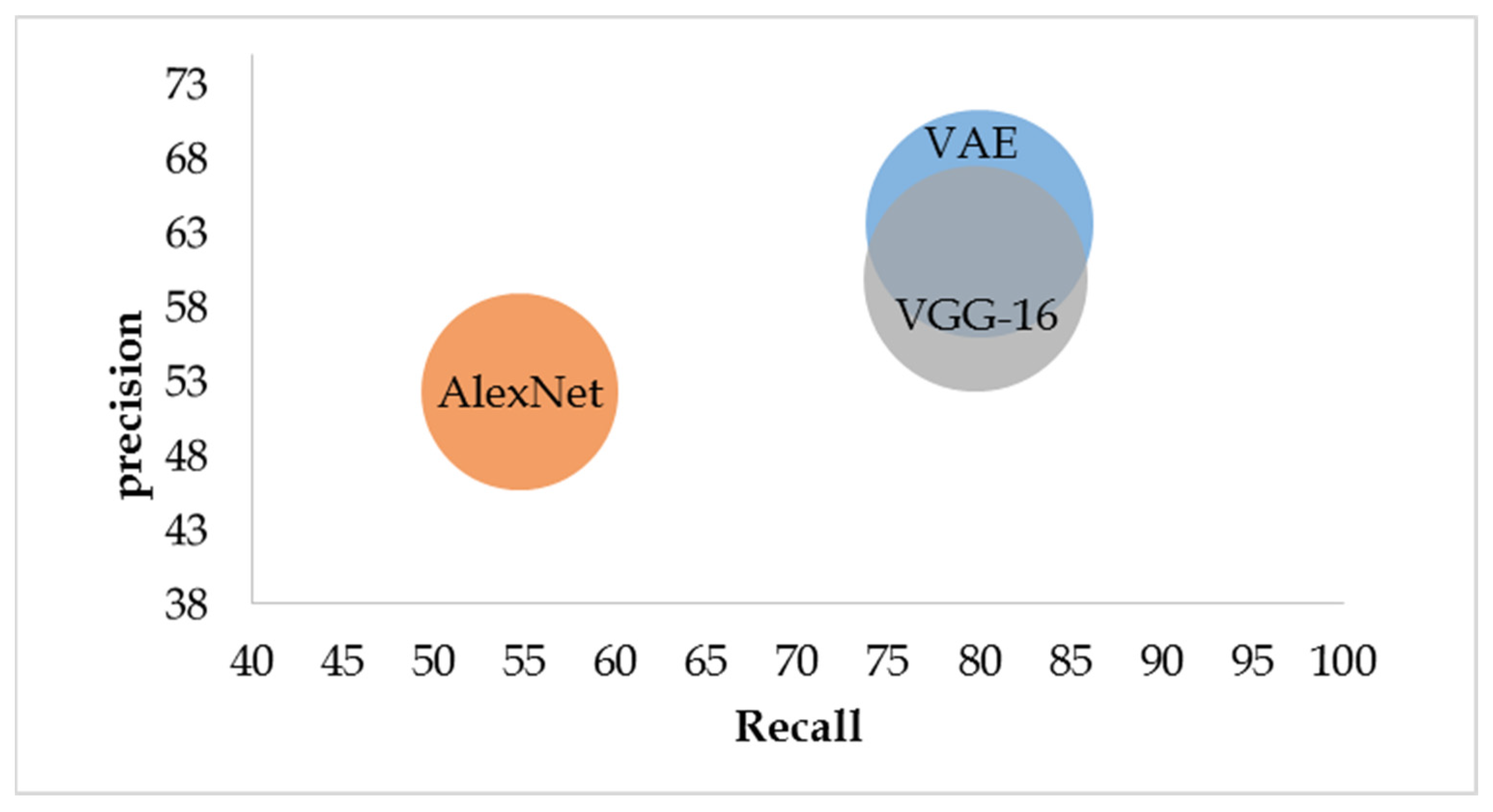
In order to demonstrate the VAE’s superiority over the CNN, a comparison was conducted with two CNN models, Vgg-16 and MobileNet. Figure 5 shows the impact of using the three models on the precision/recall of the classification results. The VAE and Vgg-16 models have close results. However, the Vgg-16 requires extra calculation time due to its number of parameters (13 convolutional layers and 3 fully connected layers).

4.1.3. CNN Hyperparameters

CNN models encompass various hyper-parameters, including the number of filters, optimizer, hidden units in the fully connected layer, batch size, and dropout rate. To identify the best hyper-parameters for the proposed CNN model in Figure 6, we employed a grid search. Table 1 presents an overview of the training, best outcomes, and their respective used hyper-parameters.
The given passage describes the process of training a CNN model on a dataset. The dataset is divided randomly into two sets: a training set (70% of the dataset) and a test/validation set (30% of the dataset). The training process involves defining input parameters such as CNN layers and training options. These include selecting an optimizer, specifying the number of iterations, and setting the mini-batch size. The CNN model learns effective characteristics over time by increasing accuracy and reducing loss. It categorizes images and identifies building classes.
Based on the results shown in Figure 7, Adamax optimizer achieved the highest accuracy of 94.98%, indicating that it is the best optimizer to use. Additionally, the best number of filters for the CNN model was 128, with an accuracy of 94.83%, while using 16 filters resulted in the lowest accuracy of 22.97%. Sensitivity analysis revealed that the optimal batch size for the model is 8, with an accuracy of 94.74%. Notably, using a batch size of 4 achieved a comparable accuracy of 94.05%. However, using batch sizes larger than 8 resulted in a significant reduction in accuracy (≃50%). Moreover, the dropout rate directly influences the accuracy of building recognition. An optimal dropout rate of 0.2 was identified, achieving an accuracy of 93.78%. The accuracy was highest when using 10 and 100 units at 83.77%, but it is believed that using fewer units in the fully connected layer enhances calculation performance, making 10 units the optimal value for this parameter.

4.2. Building Detection Results Comparison

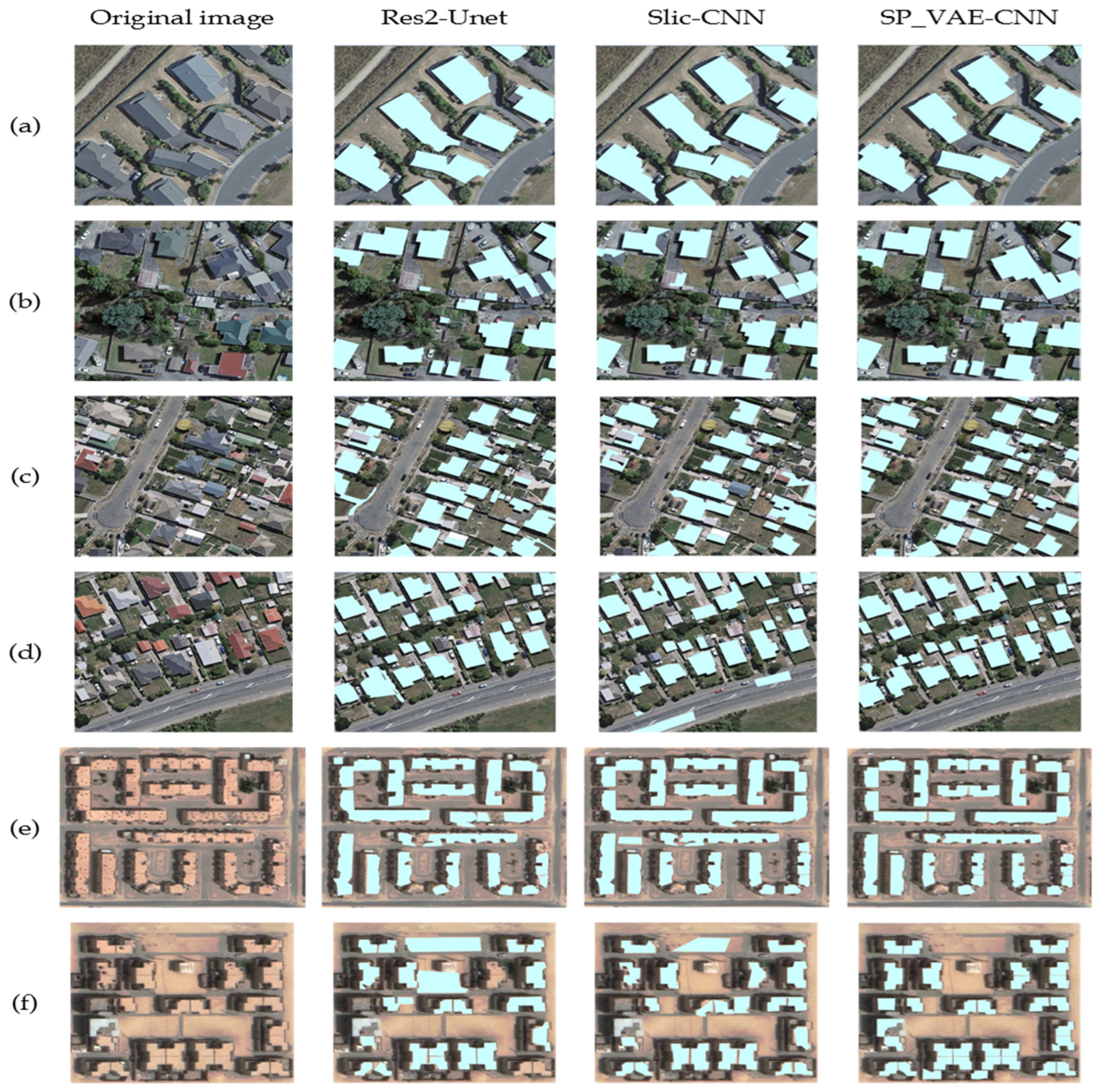
To assess the effectiveness and efficiency of our proposed approach, we compared it with the algorithms Res2-Unet [11] and Slic-CNN. To make it more challenging, images used for evaluation were carefully chosen to include buildings of varying sizes, shapes, and with roofs different color combinations. The original input images used for the evaluation are presented in the first row of Figure 8, which presents two different images from each dataset of the WHU aerial imagery 2016, New Zealand aerial image of Masterton, and Touggourt Google Earth image datasets. The final building extraction outcomes of the involved approaches are depicted in Figure 8.
Figure 8 clearly demonstrates that the other algorithms face difficulties detecting buildings with poorly defined boundaries and produce multiple missed detections. While the Res2-Unet approach focuses on building boundary correction, it requires sufficient prior segmentation, which makes it unachievable. In contrast, our proposed approach offers significant competitive advantages, particularly in terms of generalization and stability when recognizing buildings with varying characteristics. It successfully mitigates boundary errors and accurately maintains the overall building structure.
In the following experiment, five metrics were used to evaluate the performance of each approach, namely: precision, recall, F1 score, false-negative rate (FNR), and the authenticity of detection (AUT).
P = T P T P + F P
R = T P T P + F N
F 1 = 2 P R P + R
F N R = F N T P + F N
where TP (true positive) is the number of correctly detected buildings; FP (false positive) represents the number of incorrectly detected buildings. FN (false negative) stands for the number of undetected buildings. Precision is defined as the fraction of correctly predicted buildings out of all the predicted buildings, while recall is the fraction of correctly predicted buildings from the ground truth. The F1 score combines both precision and recall to provide a better understanding of how well our model is performing. Additionally, the false-negative rate (FNR) measures the degree of missed detections relative to the total number of actual buildings. Finally, the authenticity of detection (AUT) is a ratio of the correctly detected buildings corresponding to their ground truth shape.
The results shown in Table 2 demonstrate the improvement in score metrics yielded by the proposed method. It increases precision and recall while maintaining a smaller false-negative ratio compared to other algorithms, which have higher false-positive and negative rates. These findings confirm the superior feature learning ability of VAE for building detection. Furthermore, the most significant improvement was observed in the authenticity of detection, even with complex backgrounds and varying scales, sizes, and shapes of buildings, as we relied on using superpixels to accurately determine their shapes. After analyzing the results in detail, we found out that our proposed method may encounter some limitations in specific exceptional cases. For instance:
  • when shadows from other neighboring objects fall on sidewalks or driveways with similar features to the buildings they are next to;
  • when small and closely located buildings are considered one single building;
  • when shadows separate the same building into two or when trees cover parts of buildings.
Indeed, these limitations may hinder the performance of building detection methods, and it is crucial to address them in future studies.
Moreover, it is important to note that using Google Earth Satellite images for building detection may have limitations, such as image resolution and quality. In addition, the selected study area has a tropical desert climate with a building style of flat roofs, which causes the sand to accumulate on rooftops, leading to a significant similarity between the roofs of the buildings and the rest of the surrounding elements making it more challenging to identify the buildings. This explains the low results compared to the rest of the other two datasets. Nevertheless, the results obtained through our proposed approach are significantly superior to the other methods.
Ultimately, based on the tests provided, it is clear that the suggested building detection approach performs reasonably well and consistently over a wide range of complex test images.

5. Conclusions

This paper introduces a novel approach for building detection in high-resolution satellite images, named SP_VAE-CNN. The proposed approach has demonstrated impressive results, regardless of the image complexity and diversity. By combining the superpixel segmentation technique and deep learning neural network, our method efficiently reduced the computation time while maintaining high precision. The utilization of enhanced SLIC segmentation and VAE for feature extraction improved the classification performance, resulting in accurate building area identification. Moreover, our approach’s superpixels exhibited improved stability in terms of compactness and boundary accuracy, while morphology operations reduced background noise, facilitating precise building shape determination. Nevertheless, some limitations were observed in rare cases. Despite achieving high performance, further investigations are necessary for our proposed approach. These include analyzing larger and diverse datasets for generalizability, assessing computational efficiency, exploring parameter sensitivity, conducting robustness tests, and investigating methods to incorporate semantic information for improved segmentation results. These investigations will enhance the reliability and applicability of our approach.

Author Contributions

Conceptualization, A.B. and R.B.; Methodology, A.B. and B.K.; Software, A.B. and R.B.; Validation, A.B., M.-K.K. and B.K.; Formal analysis, A.B., R.B. and B.K.; Investigation, A.B.; Resources, A.B.; Data curation, A.B.; Writing—original draft, A.B. and R.B.; Writing—review & editing, A.B.; Visualization, A.B., R.B. and B.K.; Supervision, A.B. and M.-K.K.; Project administration, A.B. and M.-K.K.; Funding acquisition, A.B. All authors have read and agreed to the published version of the manuscript.

Funding

This research received no external funding.

Data Availability Statement

Not applicable.

Conflicts of Interest

The authors declare no conflict of interest.

References

  1. Sirko, W.; Kashubin, S.; Ritter, M.; Annkah, A.; Bouchareb, Y.S.E.; Dauphin, Y.; Keysers, D.; Neumann, M.; Cisse, M.; Quinn, J. Continental-Scale Building Detection from High Resolution Satellite Imagery. arXiv 2021, arXiv:2107.12283. [Google Scholar]
  2. Shen, X.; Wang, D.; Mao, K.; Anagnostou, E.; Hong, Y. Inundation Extent Mapping by Synthetic Aperture Radar: A Review. Remote Sens. 2019, 11, 879. [Google Scholar] [CrossRef]
  3. Ullo, S.L.; Zarro, C.; Wojtowicz, K.; Meoli, G.; Focareta, M. LiDAR-Based System and Optical VHR Data for Building Detection and Mapping. Sensors 2020, 20, 1285. [Google Scholar] [CrossRef] [PubMed]
  4. Hou, X.; Bai, Y.; Li, Y.; Shang, C.; Shen, Q. High-resolution triplet network with dynamic multiscale feature for change detection on satellite images. ISPRS J. Photogramm. Remote Sens. 2021, 177, 103–115. [Google Scholar] [CrossRef]
  5. Benz, U.C.; Hofmann, P.; Willhauck, G.; Lingenfelder, I.; Heynen, M. Multi-resolution, object-oriented fuzzy analysis of remote sensing data for GIS-ready information. ISPRS J. Photogramm. Remote Sens. 2004, 58, 239–258. [Google Scholar] [CrossRef]
  6. Ghandour, A.J.; Jezzini, A.A. Post-War Building Damage Detection. Proceedings 2018, 2, 359. [Google Scholar] [CrossRef]
  7. Ghandour, A.J.; Jezzini, A.A. Autonomous Building Detection Using Edge Properties and Image Color Invariants. Buildings 2018, 8, 65. [Google Scholar] [CrossRef]
  8. Aamir, M.; Pu, Y.-F.; Rahman, Z.; Tahir, M.; Naeem, H.; Dai, Q. A Framework for Automatic Building Detection from Low-Contrast Satellite Images. Symmetry 2019, 11, 3. [Google Scholar] [CrossRef]
  9. Luo, S.; Li, H.; Shen, H. Deeply supervised convolutional neural network for shadow detection based on a novel aerial shadow imagery dataset. ISPRS J. Photogramm. Remote Sens. 2020, 167, 443–457. [Google Scholar] [CrossRef]
  10. Li, J.; Huang, X.; Tu, L.; Zhang, T.; Wang, L. A review of building detection from very high resolution optical remote sensing images. GIScience Remote Sens. 2022, 59, 1199–1225. [Google Scholar] [CrossRef]
  11. Chen, F.; Wang, N.; Yu, B.; Wang, L. Res2-Unet, a New Deep Architecture for Building Detection from High Spatial Resolution Images. IEEE J. Sel. Top. Appl. Earth Obs. Remote Sens. 2022, 15, 1494–1501. [Google Scholar] [CrossRef]
  12. Yu, Y.; Li, J.; Li, J.; Xia, Y.; Ding, Z.; Samali, B. Automated damage diagnosis of concrete jack arch beam using optimized deep stacked autoencoders and multi-sensor fusion. Dev. Built Environ. 2023, 14, 100128. [Google Scholar] [CrossRef]
  13. Yu, Y.; Hoshyar, A.N.; Samali, B.; Zhang, G.; Rashidi, M.; Mohammadi, M. Corrosion and coating defect assessment of coal handling and preparation plants (CHPP) using an ensemble of deep convolutional neural networks and decision-level data fusion. Neural Comput. Appl. 2023. [Google Scholar] [CrossRef]
  14. Bai, Y.; Sun, X.; Ji, Y.; Huang, J.; Fu, W.; Shi, H. Bibliometric and visualized analysis of deep learning in remote sensing. Int. J. Remote Sens. 2022, 43, 5534–5571. [Google Scholar] [CrossRef]
  15. Mao, B.; Li, B.; Sun, J. Large Area Building Detection from Airborne Lidar Data using OSM Trained Superpixel Classification. In Proceedings of the 2019 7th International Conference on Advanced Cloud and Big Data, CBD 2019, Suzhou, China, 21–22 September 2019; pp. 145–150. [Google Scholar] [CrossRef]
  16. Cao, Y.; Huang, X. A full-level fused cross-task transfer learning method for building change detection using noise-robust pretrained networks on crowdsourced labels. Remote Sens. Environ. 2023, 284, 113371. [Google Scholar] [CrossRef]
  17. Khan, S.D.; Alarabi, L.; Basalamah, S. An Encoder–Decoder Deep Learning Framework for Building Footprints Extraction from Aerial Imagery. Arab. J. Sci. Eng. 2023, 48, 1273–1284. [Google Scholar] [CrossRef]
  18. Chen, S.; Ogawa, Y.; Zhao, C.; Sekimoto, Y. Large-scale individual building extraction from open-source satellite imagery via super-resolution-based instance segmentation approach. ISPRS J. Photogramm. Remote Sens. 2023, 195, 129–152. [Google Scholar] [CrossRef]
  19. Nurkarim, W.; Wijayanto, A.W. Building footprint extraction and counting on very high-resolution satellite imagery using object detection deep learning framework. Earth Sci. Inform. 2023, 16, 515–532. [Google Scholar] [CrossRef]
  20. Kokila, S.; Jayachandran, A. Bias variance Toeplitz Matrix based Shift Invariance classifier for building detection from satellite images. Remote Sens. Appl. Soc. Environ. 2023, 29, 100881. [Google Scholar] [CrossRef]
  21. Deng, X.; Zhang, Y.; Qi, H. Towards optimal HVAC control in non-stationary building environments combining active change detection and deep reinforcement learning. Build. Environ. 2022, 211, 108680. [Google Scholar] [CrossRef]
  22. Zheng, H.; Gong, M.; Liu, T.; Jiang, F.; Zhan, T.; Lu, D.; Zhang, M. HFA-Net: High frequency attention siamese network for building change detection in VHR remote sensing images. Pattern Recognit. 2022, 129, 108717. [Google Scholar] [CrossRef]
  23. Kusz, M.; Peters, J.; Huber, L.; Davis, J.; Michael, S. Building Detection with Deep Learning. In Proceedings of the PEARC ‘21: Practice and Experience in Advanced Research Computing, Boston, MA, USA, 18–22 July 2021. [Google Scholar] [CrossRef]
  24. Ojogbane, S.S.; Mansor, S.; Kalantar, B.; Bin Khuzaimah, Z.; Shafri, H.Z.M.; Ueda, N. Automated Building Detection from Airborne LiDAR and Very High-Resolution Aerial Imagery with Deep Neural Network. Remote Sens. 2021, 13, 4803. [Google Scholar] [CrossRef]
  25. Lv, X.; Ming, D.; Chen, Y.Y.; Wang, M. Very high resolution remote sensing image classification with SEEDS-CNN and scale effect analysis for superpixel CNN classification. Int. J. Remote Sens. 2019, 40, 506–531. [Google Scholar] [CrossRef]
  26. Sun, Z.; Liu, M.; Liu, P.; Li, J.; Yu, T.; Gu, X.; Yang, J.; Mi, X.; Cao, W.; Zhang, Z. SAR Image Classification Using Fully Connected Conditional Random Fields Combined with Deep Learning and Superpixel Boundary Constraint. Remote Sens. 2021, 13, 271. [Google Scholar] [CrossRef]
  27. Song, D.; Tan, X.; Wang, B.; Zhang, L.; Shan, X.; Cui, J. Integration of super-pixel segmentation and deep-learning methods for evaluating earthquake-damaged buildings using single-phase remote sensing imagery. Int. J. Remote Sens. 2020, 41, 1040–1066. [Google Scholar] [CrossRef]
  28. Achanta, R.; Shaji, A.; Smith, K.; Lucchi, A.; Fua, P.; Süsstrunk, S. SLIC Superpixels Compared to State-of-the-Art Superpixel Methods. IEEE Trans. Pattern Anal. Mach. Intell. 2012, 34, 2274–2282. [Google Scholar] [CrossRef] [PubMed]
  29. Vadivel, A.; Sural, S.; Majumdar, A. An Integrated Color and Intensity Co-occurrence Matrix. Pattern Recognit. Lett. 2007, 28, 974–983. [Google Scholar] [CrossRef]
  30. Bengio, Y. Learning Deep Architectures for AI. Found. Trends Mach. Learn. 2009, 2, 1–127. [Google Scholar] [CrossRef]
  31. Kingma, D.P.; Welling, M. Auto-Encoding Variational Bayes. arXiv 2013, arXiv:1312.6114. [Google Scholar]
  32. Duchi, J.C.; Bartlett, P.; Wainwright, M.J. Randomized smoothing for (parallel) stochastic optimization. In Proceedings of the 2012 IEEE 51st IEEE Conference on Decision and Control (CDC), Maui, HI, USA, 10–13 December 2012; pp. 5442–5444. [Google Scholar]
  33. Zeiler, M.D. ADADELTA: An Adaptive Learning Rate Method. arXiv 2012, arXiv:1212.5701. [Google Scholar]
  34. Kingma, D.P.; Ba, J.L. Adam: A method for stochastic optimization. In Proceedings of the 3rd International Conference on Learning Representations, ICLR 2015, San Diego, CA, USA, 7–9 May 2015; Conference Track Proceedings. pp. 1–15. [Google Scholar]
  35. Ji, S.; Wei, S.; Lu, M. Fully Convolutional Networks for Multisource Building Extraction from an Open Aerial and Satellite Imagery Data Set. IEEE Trans. Geosci. Remote Sens. 2019, 57, 574–586. [Google Scholar] [CrossRef]
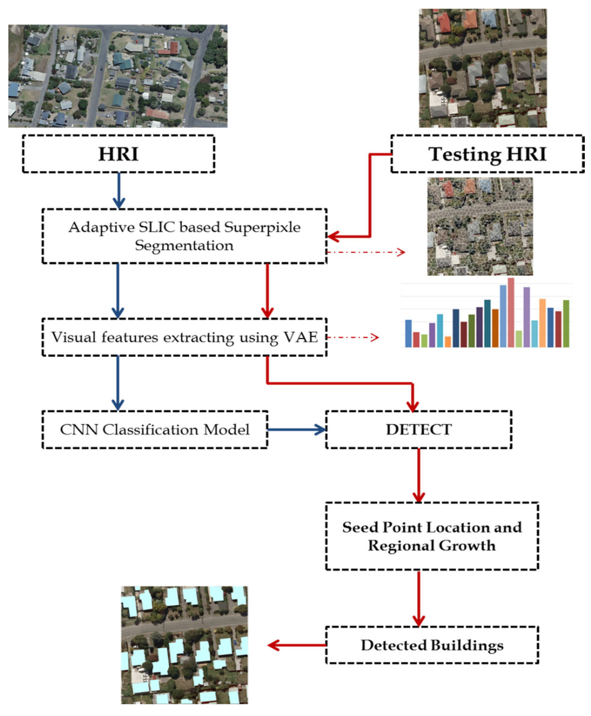
Figure 1. A general workflow of our proposed building detection method. Blue solid arrows correspond to training images, whereas the red ones correspond to test images.
Buildings 13 01649 g001
Figure 2. SLIC Segmentation results; (a) using a five-dimensional vector representation [l, a, b, x, y]; (b) using an eight-dimensional vector representation [l, a, b, e, h, c, x, y].
Buildings 13 01649 g002
Figure 3. Basic structure of a Variational Auto-Encoder.
Buildings 13 01649 g003
Figure 4. Effects of dimensionality on building detection accuracy, (a) evaluation statistics (%) IN WHU aerial imagery 2016 dataset, (b) evaluation statistics (%) IN Land Information New Zealand urban aerial image dataset of Masterton.
Buildings 13 01649 g004
Figure 5. The impact of VAE, Vgg-16, and MobileNet models on the classification results.
Buildings 13 01649 g005
Figure 6. CNN proposed module structure.
Buildings 13 01649 g006
Figure 7. The impact of CNN hyperparameters value on the accuracy.
Buildings 13 01649 g007
Figure 8. Visual comparison of aerial imagery dataset segmentation. Column 1 indicates the original input image, column 2 is the result of Res2-Unet [11]; column 3 is the result of SLIC-CNN; column 4 is the result of our proposed approach SP_VAE-CNN, (a,b) are samples from WHU aerial imagery 2016 dataset, (c,d) are samples from New Zealand aerial image of Masterton; (e,f) are samples from high-resolution Google Earth images.
Buildings 13 01649 g008
Table 1. Our Cnn’s Hyperparameters.
Parameter (Items)Search SpaceOptimal Value
Number of filters (f)16; 32; 64; 128128
number of batch b2; 4; 8; 16; 62; 64; 1288
kernel size (k)3; 55
Dropout rate0; 0.1; 0.2; 0.3; 0.40.2
number of hidden nodes (h)5; 10; 50; 100; 50010
types of the optimizer (o)RMSprop; Adagrad; Adadelta; Adam; Adamax; NadamAdamax
Table 2. Comparison of the three methods using Precision (%), Recall (%), F1-Score (%), False-Negative Rate (FNR) (%), and the Authenticity of Detection (AUT) (%).
MethodsWHU Aerial Imagery 2016 DatasetNew Zealand Aerial Image of Masterton Dataset GOOGLE Earth
PRF1FNRAUTPRF1FNRAUTPRF1FNRAUT
Res2-Unet [11]95.8395.1395.484.8790.7996.5795.1795.864.8391.1277.3281.9679.5718.0462.81
Slic-CNN92.1494.1693.145.8491.7392.8994.6993.785.3192.3569.1171.8970.4728.1144.17
SP_VAE-CNN96.7497.5797.152.4394.7697.1297.5897.352.4295.8285.8887.9586.9012.0583.37
Disclaimer/Publisher’s Note: The statements, opinions and data contained in all publications are solely those of the individual author(s) and contributor(s) and not of MDPI and/or the editor(s). MDPI and/or the editor(s) disclaim responsibility for any injury to people or property resulting from any ideas, methods, instructions or products referred to in the content.