1. Introduction
The school environment is among the most densely occupied indoor areas. Therefore, when the SARS-CoV-2 pandemic arose, the primary focus was to evaluate the infection risk in the classroom in order to balance the apparently contradictory tasks of fighting the pandemic and maintaining the fundamental service as functional as possible.
The re-opening program for schools after the so-called lockdowns shifted the focus to the safety and health conditions and, finally, ventilation.
While in the beginning there was some caution and skepticism regarding the possible airborne survival of the virus, now, this is a fact well supported by scientific evidence and studies [
1]. A consistent work [
2] analyzes the impact on infection risk (for several airborne diseases) of key different factors, such as the relative position of susceptible and infected individuals, ventilation rates and direction of air flows.
Starting from 27 February 2020, when the WHO declared that there was no proof of airborne infection for SARS-CoV-2 [
3], on 9 July 2020, the WHO declared that airborne infection was at least possible [
4], and finally, 18 months later, on 23 December 2021, it was globally admitted that airborne infection was the main infection mechanism [
5].
In order to assess the risk of contagion by air-carried particles, the Wells–Riley model [
6] was identified as an accountable predictive theoretical approach, and this was widely corroborated in the recent literature [
7]. A fundamental paper in the field of air-carried infection spread and its relation with air change rates was that by Gammaitoni and Nucci [
8], whereas other scientific investigations were published on the subject of infection risk assessment in indoor environments served with different HVAC plant types [
9]. The German virologist Christian Drosten highlighted the context of school room ventilation [
10], arguing that ventilation should be a prerequisite in order to provide healthy environmental conditions in schools.
The cited papers all agree on the fact that dilution of viral charges based on air change could be an effective means of reducing the probability of contagion. It should be emphasized that air change can be provided by:
infiltration from opening (doors and windows), generated by the inside/outside pressure gauge;
aeration generated by means of window opening due to temperature and/or pressure gauge between the outdoor environment and the room;
forced ventilation provided by an HVAC plant.
In any of the three cases above, air renewal has its effects on CO2 concentration and energy consumption:
infiltration and aeration do not control the distribution of air flows and contribute to increase the net energy demand of the building. Furthermore, they do not offer the chance for heat recovery;
regular (i.e., class change) window opening can cause rapid drops in indoor air temperature (in winter), which generates immediate (though temporary) discomfort and the need for time to restore initial conditions;
mechanical ventilation systems require energy for air displacement for a better ventilation efficiency and contaminant removal, but, on the other hand, they can offer heat recovery chance by means of heat recuperators.
Numerous papers published by ASHRAE from March 2021 to June 2021 analyze the infection risk aspects in indoor environments served by HVAC systems of the “single zone” type, both from the technical and computational points of view:
on the infection mechanism and the determination of quanta emission rates [
11];
on the distribution of aerosol [
12];
on the minimization of contagion by aerosol in environments characterized by high density occupation, adopting the model of Wells–Riley [
13].
An improved version of the Wells–Riley equation is then adopted both to account for distinct and specific scenarios of exposure to airborne pathogens and also to account for measures of protection [
14], which are
related to the specific facility, such as increased rates of air change or filters on recirculated air;
measures related to the occupant, for instance progressive levels of filtration and personal protection devices, such as masks.
In 1934, Wells proved with his extensive tests the different behaviors of liquid particles exhaled by individuals: those larger than 100 mm would fall to the ground, while the smaller ones in which the water fraction evaporated before reaching the ground were named “droplet nuclei”, and could buoy for days or at least hours [
15]. The studies of Edward C. Riley in 1978 were then aimed at developing, from an epidemiological study of a measles outbreak, an infection model for airborne diseases [
16]. Later, the model was modified according to the so-called “dose–response models” to build a consistent tool for risk assessment.
Air temperature plays a special role with respect to the biological survival rate. Lower temperatures (in the range of 7–8 °C) appear as the best boundary condition for the influenza virus; intermediate (in the range of 20–24 °C) and even higher temperature conditions (>30 °C) seem to increase the rate at which proteins and nucleic acid inactivate. At the same time, air temperature and relative humidity (RH) are quite relevant in determining the transition from droplets to droplet nuclei, since evaporation affects the falling rate. This is why there has been a significant discussion regarding the setting of a definite border to separate droplets from droplet nuclei. Finally, the World Health Organization (WHO) and the Centers for Disease Control and Prevention (CDC) set this threshold at a (mean) particle diameter of 5 mm.
The concept of quanta infection, according to the investigation on the viral charge (load) and the minimum dose able to infect others, was introduced in 1955 by Wells as the unit for measuring the infectious dose [
17,
18,
19,
20]; a “quantum of infection” is the infectious dose, which, if inhaled by a susceptible individual, is capable of inducing an infection with a probability equal to 1-1/e (circa 0.632). It must be noted that this measure has nothing to do with the number of infectious particles exhaled or inhaled. While a “well-mixed” environment condition is assumed (uniform concentration of viral quanta in a room), a backward estimation of the quanta emission from a subject who has been infected must be estimated from an outbreak case. There are also other factors that influence the spread of the disease through air, such as the survival rate, deposition rate, etc. However, this backward estimation technique considers that airborne transmission is the unique cause of all infection cases; according to those other previously cited factors, the rate can vary widely. In order to overcome the drawbacks of the Wells–Riley model, it is possible to develop dose–response models using a toxicological approach. As can be guessed, a “dose–response” model can be more flexible, but it needs dose rate data; this information is not available in the arising stages of a pandemic, and a large number of data-driven (experimental) studies are required to obtain the necessary input information to operate those models. Superspreading is thought to be a typical feature of disease spread, and it has been linked to several outbreaks, including the 2003 SARS-CoV outbreak in Hong Kong and the 2015 MERS-CoV outbreak in South Korea. Superspreading is thought to be a normal feature of disease spread; however, it is not completely understood how it works in the SARS-CoV-2 pandemic.
An environment entails complexity in terms of interactions between the occupants, appliances, furniture, the building’s physical distribution and envelope, and the climatization/ventilation system, so it is important to keep this in mind when presuming the environment is “well-mixed” [
18,
20]. Therefore, the distribution of droplet nuclei in a space can be significantly impacted by heat-generated plumes, the velocity of air supply, heat convection and human movement within the considered space. The ventilation effectiveness, which characterizes various air distribution methods, such as high induction and displacement, can be used to describe how distinct those effects are. The well-mixed assumption can produce correct results, especially when used in conjunction with mixing ventilation.
The results of the study on face mask effectiveness were quite intriguing, showing that EOC (masks assembled with three-strand non-woven polypropylene fabric), procedural and surgical masks scored efficiencies ranging from a value of 0.6 to a value of 0.9, while regular cotton knit masks had very poor efficiencies, 0.2 at most [
19]. In any situation, using braces or a fitter to improve mask sealing always increases efficiency. The reduction in infection risk brought on by masks and the same result from higher ventilation rates can be compared in an intriguing way. While an increase in mask efficiency from 0.2 to 0.6 reduces the chance of infection by an order of magnitude [
19], the ventilation rate must be at least doubled to obtain the same effect.
A recent paper from Park et al. [
21] illustrates how to use CO
2 concentration as an indicator for indoor ventilation with the aim of controlling airborne transmission of SARS-CoV-2 and other viruses.
Regarding the specific aspect of pandemic spread control in schools, a very relevant experimental study by Buonanno et al. [
22] compares the effect of manual airing and mechanical ventilation for a wide range of schools in the Marche Region of Italy; the results of the study corroborate those of the present work and those presented in the literature [
13,
14].
2. Materials and Methods
The technical requirements for school buildings in Italy were established by a National Decree from 1975 [
23], which was withdrawn in 1996 but is still cited. For the present purposes, this work specifically refers to [
18]:
the floor area per single occupant/pupil;
the window area divided by floor area, for daylighting purposes;
and the basic thermal comfort parameters (air temperature and relative humidity variation range, which have to be controlled through ventilation).
However, the ventilation systems in Italian school buildings are quite poor. Although they may exist in some regions and in new constructions, these systems are frequently of the air recirculation type, which has its own well-known negative qualities [
9].
According to various school classes, the window area per floor area should be between 1/7 and 1/5, whereas the pavement area per person varies in a range between 1.8 and 2.0 m
2 [
18].
The primary objective of the paper is to compare the effects of infiltration, aeration or ventilation in a classroom from the perspectives of energy and infection risk assessment.
The assumption of an ordinary school room is the one derived from the requirements set out by the Italian Decree [
23] for a class of 25 students and serves as the starting point. The minimum floor size required by the decree is equal to 49 m
2, and 10 m
2 in terms of the window area is sufficient to meet the most stringent 1/5 ratio between the window area and the floor area. With a ceiling height of 3 m, the consequent volume of the room is 147 m
3 [
18].
In order to incorporate window opening (aeration) and infiltration, a simplified model was created. A “well-mixed” model of air in a space takes into account the heating system’s contribution, as well as heat transfer from the walls to the surrounding air. The initial air and wall temperatures are both 20 °C.
The internal surface/wall temperature follows the model of a semi-infinite wall and is determined by the fixed convection coefficient of 10 [W m
−2 K
−1], according to the following formula [
24]:
Formula 1. Model for semi-infinite wall temperature response.
Let
x [m] be the considered depth,
t the time [s] and
Diffusivity is assumed as 8 × 10
−7 [m
2 s
−1] [
18].
Thermal diffusivity
a =
λ/(
r ·
c) is determined by assuming the average values for thermal conductivity of 0.8 [W m
−1 K
−1], specific heat of 1 [kJ kg
−1 K
−1] and density of 1000 [kg m
−3], typical of the building materials in the literature [
24].
The complete interior physical boundary of the space, excluding the wall with windows, is used to calculate the heat transfer surface area, which is 106.35 m2. The adoption of the semi-infinite wall model step response might not be the most accurate strategy to describe the system, and a numerical simulation could be a better choice. However, one must account for:
the computing time optimization in multiple runs, which is dramatically shorter for the adopted model versus a numerical simulation with the transfer function method;
the contribution of heat transfer from the walls to the air, which in the first law balance of the environment is at least one order of magnitude smaller than those from incoming outdoor air or from the heating system for such short transients (5′ or 10′).
Therefore, the adoption of the model, considering average values for thermal transmittance and capacity among the different surfaces of the envelope, is considered sufficiently accurate in order to model the described event.
The heating system’s (radiators) contribution is computed using a peak power of 3.41 kW at winter outdoor design air temperature [
23], which equates to a main supply hot-water temperature of 75 °C, and decreases using the UNI EN 442 formulae, taking into account a bottom supply temperature of 55 °C corresponding to an outdoor temperature of 16 °C. A further contribution from the heating system is not present if the outside temperature rises over 16 °C.
In order to calculate an approximate air flow from window opening [m
3 s
−1], the model of UNI EN 16783-7:2018 [
25] was taken as reference, with the subsequent formula (44)
Formula 2. Window-opening-generated air flow formula.
In the formula, let hw be the height of the center of the window assumed to be equal to 1.5 m; Cst is the coefficient, which accounts for the stack effect in the calculation of air change and is equal to 0.0035 [s−1 K−1]; and Cwnd is the coefficient, which accounts for the wind speed and is equal to 0.001 [s m−1].
The numerical integration of the problem can be listed as follows:
t = 0, Formula 2 with T = 20 °C → air flow Q [m3 s−1] of outdoor air incoming at temperature Te (which will occur in the first time step of 1 s);
t = 1 s, first law balance for air temperature gives the amount of heat removed from the environment due to the air change qac;
t = 1 s, Formula 1 with T = T’ and Y = 0 (for x = 0) returns surface wall temperature Tf;
the heat released from the walls to indoor air is calculated by means of a convective balance qw = a (Tf − T);
the heat from the radiators’ heating system is determined according to the standard EN 442:2015 [
26] (or similar indications from the manufacturers’ handbook)
qr =
qnom ((
Tw −
T)/50)
1,33, where
qnom is the rated heating capacity (2 kW for the location of Padova, then adjusted according to the design temperature for other locations), and
Tw is the average water temperature in the radiators.
Tw is determined from
qr =
m c (
Ts −
Tret), i.e.,
Tw = (
Ts +
Tret)/2, where m is the radiators’ mass flow, and c is the water specific heat;
Ts is the radiators’ supply temperature, and
Tret is the radiators’ return temperature.
Ts is a linear function of outdoor air temperature (75 °C at outdoor design temperature and 55 °C at 16 °C outdoor temperature). This calculation is only performed in the first time step; then, given the slow change in outdoor air temperature, the heat from the radiators is considered constant;
the sum of qac + qw +qr is the total amount of heat exchanged from indoor air; then, the final temperature of indoor air is calculated by the first law balance.
The calculation is then repeated until the end of 300 steps (5 min) or 600 steps (10 min); at the end, one will obtain T (the final temperature of indoor air), the sum of heat released from the walls to the air and the sum of heat due to air change; the plant must re-supply both of them to restore initial indoor conditions.
While CIBSE [
27] also presents a method for estimating infiltration, in this case, the air flow through infiltration is computed in accordance with UNI EN 12207:2017 [
28] for various categories of air tightness in windows. Class 1 means 75 m
3 h
−1 of air infiltration for the aperture of 10 m
2 assumed in this work, while class 2 means 39.9 m
3 h
−1.
From 15 September to 15 June—which includes the whole winter season—the school facility is thought to remain open from 8 am to 1 pm, five days a week. The official UNI-CTI database [
29] was used to estimate the hourly weather data. Several Italian places were chosen as listed below [
18]:
- -
Padova, with an average wind speed of 2.1 m s−1 and 2383 heating degree days (HDD), winter design temperature −5 °C;
- -
Torino, with an average wind speed of 0.9 m s−1 and 2617 heating degree days (HDD), winter design temperature −8 °C;
- -
Roma, with an average wind speed of 1.3 m s−1 and 1415 heating degree days (HDD), winter design temperature 0 °C;
- -
Napoli, with an average wind speed of 3.2 m s−1 and 1034 heating degree days (HDD), winter design temperature +2 °C;
- -
Palermo, with an average wind speed of 0.9 m s−1 and 751 heating degree days (HDD), winter design temperature +5 °C.
The mask efficiency was assumed to be constant and equal to 0.5; while this is an average-to-poor value when set against those analyzed in ref. [
14], it also takes into account adjustments due to non-hermetic sealing provided by the ability to wear a mask properly, as strict adherence to the instructions is unlikely to be continually upheld in schools.
In order to fall between class 1 and class 2, as per the infiltration rate of the glazing systems, a value of 60 [m3 h−1] was assumed.
A pupil carrying the infection would emit 8 quanta per hour, while the instructor would emit 50 quanta per hour. The COVID-19 Delta variation, which was prevalent in the latter pandemic period, is said to be a little more contagious than the other variants; thus, these figures are a little higher than those in the literature.
Since the exposed subjects cannot be assumed to be uniformly susceptible—some of the students may be immunized or may have previously contracted the disease, for example—it is much preferable to provide the “individual probability of infection”
P in this study, as opposed to previous ones, which take the reproduction index into account, such as
R* in ref. [
9].
P indicates “fully susceptible individuals”, since people who experience partial immunization react differently and less severely to infectious situations.
All calculations were conducted assuming a “well-mixed” [
9] and “perfectly and instantaneously mixed flow” in the room. Therefore, when the windows are open, the virus (or other gases, such as CO
2) concentrations in the indoor air are estimated by instantaneous blending with the incoming fresh outdoor air. Therefore, the estimated results could eventually produce conclusions, which are more constricted than what is actually true.
The question of the likelihood of infection for a single completely susceptible pupil exposed to multiple successive identical events (
N) every day arises because the school is attended with daily frequency. The likelihood of
N independent events can be calculated using the formula below:
This is the same outcome, which is achieved if the calculation is performed with respect to the sum of infection doses that are inhaled in total during the period, if the probability is computed according to the Poisson formula (Wells–Riley) for evenly probable events [
19].
In order to calculate the CO
2 concentration, a respiration-related concentration increase of 38,000 ppmv [
19] (concentration in the exhaled air minus concentration in the inhaled air) is assumed [
30].
3. Results of the Calculations
This section is split into two subsections. The first subsection focuses on the thermodynamic and energy effect of opening windows versus mechanical ventilation, while the second subsection focuses on the likelihood of disease spread for both containment strategies using window opening and mechanical ventilation.
3.1. Air Change through Window Opening and Room Temperature
It is believed that window opening will most likely take place at the conclusion of each class hour, based on a typical working schedule of a school. A few simulations were performed using two sample times of window opening, 5 min (300 s) and 10 min (600 s), since these are the times likely available for class change.
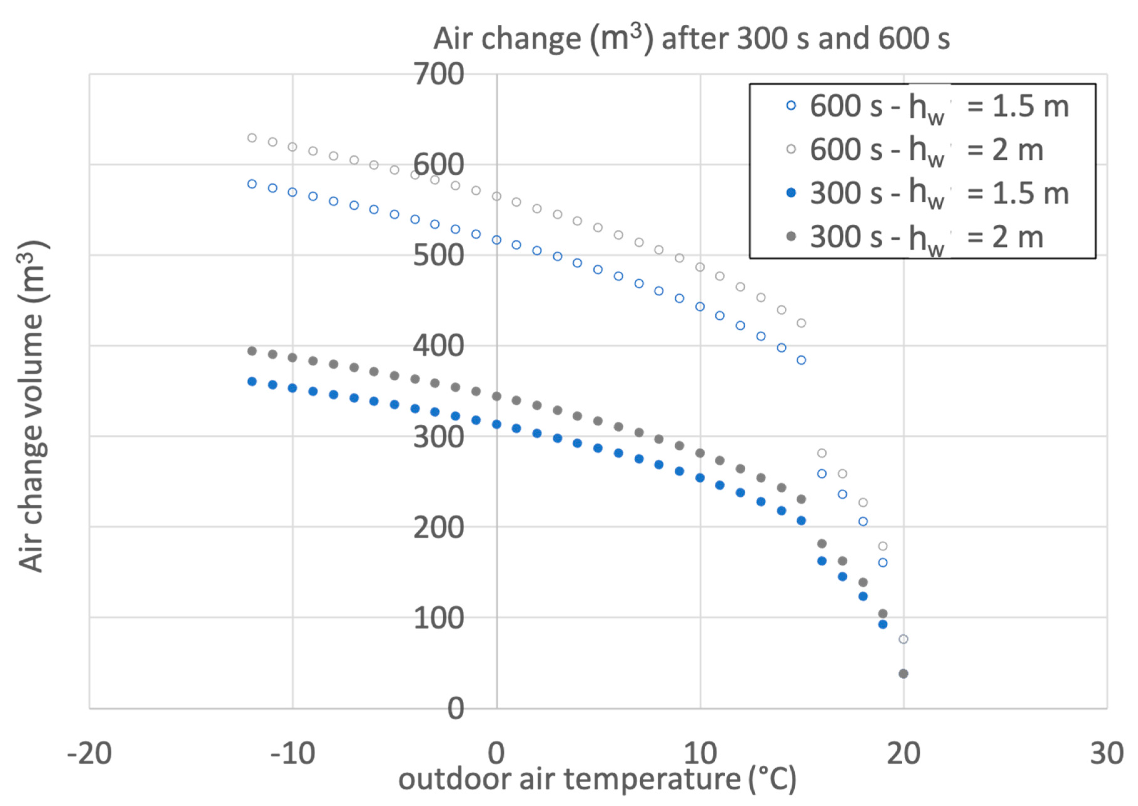
The initial calculations assume that only half of the window surface, i.e., 5 m2, is open, with the center of window opening at 1.5 m, i.e., hw = 1.5 m, and the initial indoor air temperature at 20 °C, i.e., Ti = 20 °C, according to Formula 2 nomenclature.
Figure 1 depicts the total (obtained by numerical integration of Formula 2 at 1 s resolution) volume of air change after 5 min and 10 min for different mean values of wind speed values and outside temperatures. It appears that only at moderate outdoor temperatures can the effect of the different wind speeds change the outcome, and that once the opening time is doubled, there is no doubling of the air change volume (except for high wind speeds, such as 8 m/s). Due to the shape of the expression in Formula 2, the effect of wind speed at lower velocities does not affect the air change, except at mild temperatures.
In
Figure 2, the final room air temperature is shown for several values of mean wind speed and outdoor air temperatures after 5 min and 10 min of window opening with the same values of
hw (1.5 m) and
Ti (20 °C) adopted for the previous simulation. As can be seen, at mild outdoor temperatures, modest changes caused by wind speed can be noticed; however, the impact of heating shut-off can be felt more strongly above 16 °C. The discontinuity is due to the form of the expression in Formula 2.
As can be seen from the plots, the effect of doubling the open window area does not equate to doubling the window opening duration, as can be observed in
Figure 4 and
Figure 1.
Then, in order to get a better grasp of the issue, several computations were performed.
Figure 5 details the effect of the initial indoor air temperature on the total air change at the end of the 5 min and 10 min window opening time. The discontinuity is due to the form of the expression in Formula 2.
Energy and HVAC Calculations
It is intriguing to think about how the air change estimates may affect the room’s net energy requirements. The total amount of thermal energy needed, generated by window opening, is the sum of the thermal energy needed to recover the initial air temperature
Ti and that needed to recover the initial indoor walls’ temperature
Ti; this second term is the integral of the thermal power released into the air from the walls (see
Section 2).
This thermal energy net demand (which must be supplied by the heating and cooling plant) for window opening and infiltration is then compared to the amount of thermal energy net demand induced by a forced mechanical ventilation system, which supplies/extracts an air flow of 735 m
3/h [
18] (
rn of 5, according to the law [
23]). The system is considered to be equipped with a heat recuperator, which scores an efficiency (referred to as sensible heat) of 75%; the electric consumption of the ventilation equipment is 180 W.
Without taking into account the efficiency of the heating and cooling plant (which is invariant for the problem posed), on the one hand, there is a thermal need for initial conditions’ recovery (energy lost from window opening, both from outside and from the wall side), and on the other hand, there is a thermal need to supply “neutral air”, which comes out of a cross flow heat recuperator. Since the efficiency of the recuperator is 75%, the sensible energy demand will be roughly a quarter of the sensible energy flow associated with the supply air flow.
Again, it has to be remarked that the comparison is based on AHU terms, at a fixed renewal rate rn of 5, while in the “window opening” scenario, this renewal rate varies according to the outdoor air conditions on an hourly basis.
According to the presumptive scheduling, the system is thought to be operational 1206 h every year. The findings are described in
Table 1 below (already presented by the same authors in [
18] and further developed in the present work), taking into account the opening of a 10 m
2 window glazing for an interval of 300 s at the end of every class period.
As can be seen, although never supplying a rn above 2, the winter loss from window opening and infiltration can total more than 2000 MJ. On the other hand, mechanical ventilation (AHU), which offers a rn of 5, results in a heat demand of 2300 MJ. The amount of electricity used per year is 217.1 kWh.
3.2. Infection Risk Assessment
The calculation of the infectious quanta concentration trend over time is thoroughly explained in ref. [
8]; the Wells–Riley model used to calculate each person’s chance of infection P is also covered in great detail in the same source. There are also some removal factors to be considered, which are given the following values in accordance with ref. [
3]: by deposition
k = 0.24 h
−1; by viral inactivation
λ = 0.63 h
−1 [
19,
20]; as per the infectious quanta present in the indoor environment, their initial level is considered to be 0 corresponding to
t = 0. The window opening events occur at the conclusion of each class hour.
To implement the mathematical modeling and to then compute the results based on the presumptions stated, a code was created in a commercial computing Calculus environment.
The mathematical model is based on the Wells–Riley equation [
16], which gives the probability of a susceptible individual contracting a disease via aerosol infection. This follows a Poisson probability function according to Formula 3:
Formula 3. Wells–Riley probability model.
Lately, Gammaitoni and Nucci [
8] derived an expression for calculating the viral concentration C, assuming the following simplifying assumptions: the quanta emission rate is considered constant over time; the latent period of the disease is longer than the time scale of the model; and the droplets are distributed instantaneously and uniformly in the room. This equation is written considering the “total removal factor”
trf and considering all factors contributing to viral load removal in the room volume (deposition, inactivation and air renewal) as follows:
Formula 4. Gammaitoni–Nucci formula.
Formulae 3 and 4, from
n0 = 0 yield to the probability of infection for a susceptible individual, are as follows:
Formula 5. Probability of infection for a susceptible individual.
The initial findings compare the levels of infectious quanta [
20] in the classroom among students wearing or not wearing masks; the quanta are diluted with air penetration only, and a single student is assumed to be infected. The picture captions also state that after a 5 h class, the individual risk of infection is equivalent to 0.16 without a mask and 0.044 with it, demonstrating a 4× risk reduction as a result of mask use (
Figure 6).
The findings are reported in the second set of plots using the same fundamental assumptions, but in this case, the environment is equipped with a forced ventilation system providing 40 m
3/(h person) of fresh outdoor air. With mechanical ventilation, the individual infection probability decreases from 0.16 to 0.033 without a mask, and from 0.044 to 0.0083 (
Figure 7) with a mask. This is close to a five-fold reduction figure or a half order of magnitude. According to a comparison of the plots in
Figure 6 and
Figure 7, masks can not only be replaced but even outperformed by mechanical ventilation.
The final set of findings in
Figure 8 illustrates the impact of manually opening the windows for aeration. An aeration air change of 200 m
3 for a 5 min opening duration was chosen as the average figure from the previous section of the study. The comparisons made between
Figure 7 and
Figure 8 illustrate how mechanical ventilation causes the individual infection probability to decrease by a factor of 3 (at least) both with and without mask use in comparison to natural ventilation by infiltration alone.
The above conclusions only apply to exposure to a polluted environment during the five hours of daily teaching and are based on a single day event. The same condition can occur repeatedly if there is an asymptomatic spreader always present. The plots in
Figure 9 deal with this situation. For the purpose of conciseness, and because mechanical ventilation systems are rarely installed in Italian schools, only the case of infiltration and manual aeration is taken into consideration. As can be observed, the impact of the quantity of air provided by aeration is enormous; if manual aeration is limited owing to environmental factors or brief window openings, the risk of infection can rise significantly by practically a factor of 2. Mask use, as anticipated, reduces the risk of infection by a factor of 4.
When extending the presence of infected people to more days (i.e., in a likewise case of an asymptomatic), the consideration regarding the probability of contagion from multiple events must be recalled from
Section 2, as follows:
Formula 6. Probability of infection from multiple events.
A fifth set of data takes a different scenario into account: the instructor is sick (instead of one student), with infiltration and aeration through windows.
Figure 10 and
Figure 11 show the plots and inscriptions, which illustrate this condition.
It should be emphasized that under the current Italian law, vaccinations are not permitted for those under the age of 12. In this scenario, all pupils in primary and secondary schools may be viewed as entirely susceptible. In this instance, the reproduction index R* calculation demonstrates that, even with a full mask on, an infected teacher can still infect at least one student after a two-hour class; however, in the absence of mechanical ventilation, an infected instructor could infect between three and six pupils without a mask.
CO2 Concentration
Additional calculations were performed to determine the CO2 concentration trend over time in a classroom with infiltration and manual aeration.
The calculations were performed in a commercial computing Calculus environment. Those calculations account for
Emission of metabolic CO2 from occupants;
Air renewal through window opening and infiltration;
Outdoor CO2 concentration of 400 ppm.
These simulations continue to operate under the premise of perfect mixing. The curve in
Figure 12 demonstrates how infiltration is unable to sustain the desired CO
2 concentration of 1000 ppmv due to a lack of air change. The expected manual aeration through opening windows is unable to lower this value below 1000 ppmv at the end of each opening, and the CO
2 concentration quickly approaches 1000 ppmv shortly after arrival.
Figure 13 shows how the average value for concentration of CO
2 in 5 h classes cannot possibly be maintained under 2000 ppmv, even at the maximum possible rate of aeration (350 m
3 in 5 min).
These findings regarding a trend in indoor CO
2 concentrations appear to be very similar to the experimental data reported in ref. [
31], despite the fact that due to some differences in the ways the problems are dealt with, a comparison is not possible.


