Discussion on Calculation Method of Magnification Factor of Toggle-Brace-Viscous Damper

Abstract

At present, dampers are widely used in the field of energy dissipation in engineering structures. However, when the displacement and velocity output of dampers are not significant under small and medium-sized earthquakes, it is difficult for a damper to fully exert its energy dissipation capacity. The use of toggle-brace mechanisms in the structure is an effective method to solve the above problems, and the effect of toggle-brace-viscous dampers (referred to as TBVDs) in the structure can be reflected by a magnification factor (referred to as M_f). Therefore, it is particularly important to study the calculation method for the M_f of TBVD. Domestic and foreign scholars have achieved certain results in the study of the calculation method for the M_f of TBVD, and the corresponding calculation formula for the M_f has been proposed. Given the existing research results, this article conducts the following work: analyzing the shortcomings of existing methods for calculating the M_f of TBVD, proposing an improved method for calculating the M_f of viscous dampers, comparing the accuracy of existing and improved algorithms, and analyzing the calculation results to provide practical suggestions for engineering applications.

1. Introduction

In recent years, a significant number of casualties and property losses have been documented and reported [1,2,3,4,5] as the impact of earthquakes becomes more frequent. The main causes of these disasters can be attributed to two factors: higher seismic magnitudes and a lack of awareness among design professionals regarding seismic design principles, which can lead to unfavorable phenomena such as “strong beams and weak columns” and “under-reinforced beams and columns” in structures. Traditionally, increasing structural stiffness has been considered an effective means of improving the overall seismic resistance of a structure. An increase in structural stiffness enhances the corresponding seismic capacity, but higher stiffness hinders the rational dissipation of energy. For frame structures, the use of dampers for energy dissipation is regarded as an effective measure to address the issues [6]. When a frame structure is subjected to earthquake action, the input energy is primarily dissipated by the installed dampers; subsequently, the remaining energy is consumed by the frame. The effectiveness of energy dissipation is reflected in the attenuation of overall structural damage [7,8,9,10]. Dampers can be classified into two categories based on their operating principles: velocity-based dampers and displacement-based dampers. The energy dissipation capacity of the former is mainly dependent on the velocity magnitude, with higher damper forces generated by faster deformation velocities, such as viscous dampers and viscous damping walls. The energy dissipation capacity of the latter is primarily related to the displacement magnitude. These dampers not only possess certain stiffness adjustment capabilities but also provide additional damping ratios, such as buckling-restrained braces [11] and metal dampers [12], etc. Compared to the latter, viscous dampers in the former category can provide damper forces to the structure without increasing stiffness, thereby demonstrating more significant advantages over other types of dampers [13].

In newly constructed and existing frame structures [14,15] and frame-shear wall structures, viscous dampers possess numerous advantages, including high installation rates, large numbers installed, and significant seismic performance. Wall-type connections, diagonal connections, and chevron connections are employed when there is a relatively large inter-story displacement in the structure. Conversely, viscous dampers with amplification devices are used when the inter-story displacement is relatively small. Among various types of viscous dampers, toggle-brace connections create a “cycle closure” effect in the supporting components, effectively controlling the dynamic response of the structure through the reverse (inhibitory) action of the large displacement output from the viscous dampers [16,17,18,19].

Imitating the principles of linkage mechanisms in mechanical engineering, elbow-joint support connection devices were proposed by Constantinou et al. [20], which can provide a larger usable space below upon installing its ends at the beam-column joint positions of the frame. At the same time, this elbow-joint support possesses numerous advantages, not limited to the following: compact dimensions of the installed members, a large displacement amplification factor, stable and secure node connections, controllable out-of-plane instability, and so on. Reports in the literature [20] indicate that toggle-brace connections exhibit superior seismic performance compared to other forms of damper connections, effectively controlling the dynamic response of the overall structure when subjected to earthquake action or wind and snow actions. Furthermore, simulation results validate their significant effectiveness in energy dissipation [21].

A significant displacement amplification effect of a frame structure equipped with dampers and amplification devices under earthquake action was reported in the literature [20] through the shaking table test. For TBVDs without bending action, the M_f can be used to quantify the effectiveness of the damping effect. The reasonable optimization of the M_f is achieved through theoretical derivation and comparative analysis. The derivation formula for the M_f of TBVDs was proposed in the literature [20], but its validity and accuracy have not been effectively verified.

Based on the aforementioned background, the main objective of this study is to explore and improve the calculation method for the M_f of TBVDs. The study is divided into three parts: the first part provides a detailed exposition of the existing theoretical framework; the second part focuses on addressing the deficiencies and limitations of the existing theory; and the third part involves practical verification of the feasibility and accuracy of the proposed improved method.

2. Introduction of Improved Algorithm

2.1. Existing Algorithm

The schematic diagram of the toggle-joint support and corresponding frame system is shown in Figure 1. The TBVD is installed at a specific position within the frame, consisting of two toggle-joints support and one viscous damper. One end of the viscous damper is installed at the rotatable toggle joint, and the other is installed on the node plate of the beam-column. When inter-story displacement occurs in the frame, the rotation of the toggle-joint support causes the viscous damper to undergo expansion and contraction deformation, which results in a relative displacement at both ends of the damper greater than the inter-story displacement of the frame. The formula proposed in the “Technical specification for seismic energy dissipation of buildings” (JGJ 297-2013) [22] is used to quantify the energy dissipation capacity of viscous dampers (W_cj = λ₁F_djmaxΔu_j). When using toggle support and conventional support within a specific span, by using toggle-joint support and conventional support within the same span, the damper force of both can be considered close due to their close translational velocity. It can be seen that the energy dissipation capacity of the two supported dampers is only proportional to the displacement and motion of the two ends of the damper. Due to the fact that the M_f can be used to quantify the displacement and motion of both ends of the viscous damper, the energy dissipation capacity of different types of dampers can be represented by the M_f.

For the convenience of theoretical analysis and common formula derivation, considering the deformation capacity of the toggle joint-supported damper frame system under earthquake action, the following six assumptions are given based on the relevant literature [16].

(1)

The frame only performs rigid body motion;

(2)

The floor height remains unchanged when the column rotates;

(3)

The length of the toggle-joint support is fixed and considered a rigid connecting rod;

(4)

Additional dampers can freely contract along the axial direction;

(5)

The floor slab has absolute stiffness, and the stiffness ratio of the beams and columns is infinite;

(6)

The influence of the connection method between beams and columns on the deformation of dampers can be ignored.

Under the above assumptions, the M_f of the toggle-joint support damper is derived as follows. Firstly, the lateral deformation of the frame under lateral force is analyzed; Secondly, the geometric relationships of the components of the toggle-joint support system before and after rotation are clarified, as shown in Figure 2; Finally, the M_f suitable for the toggle-joint support damper is formed through reasonable simplification, as shown in Equation (1).

$$f=\frac{\cos {\theta }_1}{\cos ({\theta }_1+{\theta }_2)}-\cos {\theta }_2$$

(1)

where θ₁ is the angle between the upper toggle brace and the beam, and θ₂ is the angle between the lower toggle brace and the column. According to the formula, the M_f is only related to θ₁ and θ₂, independent of the overall structural lateral displacement. In practical engineering, the span and story height are first determined, the angle between the toggle brace and the frame is then obtained, and the M_f is ultimately calculated. However, the process of solving the M_f is relatively complex, leading to the lack of availability in practical engineering. In order to maximize the convenience of calculating the M_f and the universality of engineering applications of TBVD, it is necessary to improve and simplify the existing theoretical formulas.

2.2. Improved Algorithm

The schematic diagram of the TBVD support system without bending is shown in Figure 3. The geometric dimensions of the frame are as follows: the height and width are h and l, respectively. The lengths of the two support rods are l₁ and l_2, respectively, and the angle between the damper and the column is α. The effect of earthquake action on the frame is similar to the effect of lateral displacement (u) on the frame. When the length of the viscous damper before and after deformation and the lateral displacement of the frame vertex are determined, the M_f can be calculated. The specific calculation method for deriving the coordinates of the damper before and after deformation through geometric relationships is as follows.

The deformation of the TBVD is shown in Figure 4. The upper and lower toggle brace rotate around points A and B, respectively, and the rotational effect can be seen as indirectly amplifying the deformation of the damper. When calculating the deformation of the damper, the following assumptions are considered: (a) the length of the upper and lower connecting rods is fixed when encountering earthquake action; (b) the stiffness of the frame beam is infinite; (c) the changes in the elevation of the frame can be ignored. Under the condition that the frame is not subjected to horizontal displacement, points B and F are the two ends of the lower toggle brace, respectively; Points A and F are the two ends of the upper toggle brace, respectively; Point C and D are the beam-column nodes, respectively; Point B and point E are the lower endpoints of the column, respectively. When the frame undergoes lateral displacement (u), points A, C, D and F are converted to A’, C’, D’ and F’. Although the ordinates of these points remain constant, the corresponding abscissa increases by u. The geometric relationship between point F is as follows: the distance between point F and point A is l₁, and the distance between point F and point B is l₂. The abscissa and ordinate of point F are set as x₁ and y₁, respectively. x₁ and y₁ are presented in Equations (2) and (3). Given the coordinates of points F and A, the length of l₁ can be calculated, as shown in Equation (4). The abscissa and ordinate of point F’ are set as x₂ and y₂, respectively. When geometric relationships are quantified, a system of binary quadratic equations can be established. The coordinates of the damper after deformation can be calculated by solving a system of binary quadratic equations. This geometric relationship is presented in Equations (5) and (6).

$$x_1=h\times \cos \alpha \times \sin \alpha$$

(2)

$$y_1=h-h\times {\cos }^2\alpha$$

(3)

$$l_1=\sqrt{{(0.5\times l-x_1)}^2+{(h-y_1)}^2}=\sqrt{{(0.5\times l-h\times \cos \alpha \times \sin \alpha )}^2+{(h\times {\cos }^2\alpha )}^2}$$

(4)

$$x_2{}^2+y_2{}^2=l_2{}^2={(h\times \sin \alpha )}^2$$

(5)

$${(x_2-0.5\times l-u)}^2+{(y_2-h)}^2={l_1}^2$$

(6)

The coordinates obtained from the above equations are the position of the damper after deformation. The position of the damper before deformation can be derived based on geometric relationships. The length of the damper before and after deformation can be obtained according to the definitions shown in Equations (7) and (8).

$$u_{D1}=\sqrt{x_1{}^2+{(y_1-h)}^2}=h\times \cos \alpha$$

(7)

$$u_{D2}=\sqrt{{(x_2-u)}^2+{(y_2-h)}^2}$$

(8)

In the formula, u_D1 is the length of the damper when the frame has not been subjected to an earthquake, u_D2 is the length of the damper after the frame has been subjected to an earthquake, and u_D is the deformation of the damper. The displacement generated by the deformation of the damper is represented by Equation (9), and the M_f is the ratio of the damper deformation to the displacement between the adjacent floors, as shown in Equations (9) and (10).

$$u_D=\left|u_{D1}-u_{D2}\right|$$

(9)

$$f=\frac{u_D}{u}$$

(10)

2.3. Implementation of Improved Algorithms

As a widely used programming language, Python is not only a Scripting Language but also a Glue Language. By using source code and APIs, programmers can write modules within software such as C, C++, and Python. Compared to other programming languages, it has advanced data structures. Python is not only seen as a concise and easy-to-learn language but also as a concise and efficient data processing tool. The function of Python’s Numpy module is similar to that of MATLAB. Both of them have powerful data processing capabilities, but the running program of the former is smaller than that of the latter. Due to the many advantages of Python software, data in this article were processed using Python software.

The core of this algorithm is to obtain the solution of the aforementioned binary quadratic equation system, which is defined as the coordinates of the viscous damper after the frame undergoes deformation. Due to the phenomenon of unknown high power and coupling between two unknowns in the equation system, the M_f of the damper is calculated using a script formed by the Python module. The required input parameters for this script are story height h, span l, relative displacement u, and the angle between the damper and the column α. The Python code can be found in Appendix A.

3. Modeling Program

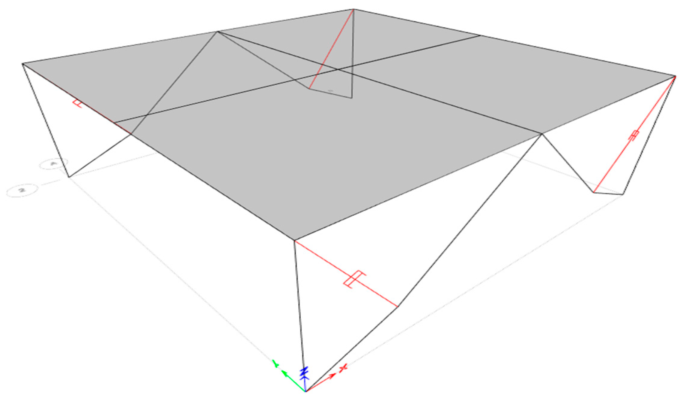
3.1. Model Overview

To investigate the effects of story height and span on the M_f of a single-story single-span frame structure and to explore the variations of M_f for structures with small inter-story drifts (where the inter-story drift angle is less than 1/800 during frequent earthquakes), this study designed nine sets of models, as detailed in

Table 1. Dimensions of the model.

Model	Height (mm)	Span (mm)
Model-1	4000	8000
Model-2	4000	10,000
Model-3	4000	12,000
Model-4	5000	8000
Model-5	5000	10,000
Model-6	5000	12,000
Model-7	6000	8000
Model-8	6000	10,000
Model-9	6000	12,000

. All models adopted single-story and single-span frame structures with TBVD arranged only in the x-direction. To facilitate the application of vertical floor loads, the models considered the design of floor slabs. Secondary beams were incorporated into the models to reduce the deflection of the primary beams. Vertical loads were transmitted from the floor slabs to the main and secondary beams, then transferred to adjacent columns, and ultimately transmitted to the ground. No ground beams were designed at the base of the columns; only fixed-end supports were provided. The arrangement details of the models and TBVDs are shown in Figure 5.

3.2. Model Design

The ETABS finite element analysis software was utilized to analyze the energy dissipation and deformation of TBVD. In the process of model creation, fiber beam elements were employed for beams and columns, thin shell elements were utilized for floor slabs, rigid connections were adopted for beam-column connections, and the ends of the link elements were fully released in the local axis (3) direction to simulate hinges.

The beams and columns are both designed with rectangular cross-sections made of reinforced concrete. The elbow-joint supports employ H-beam steel sections, with detailed parameters listed in

Table 2. Design parameters of the model (unit: mm).

Part	Section
Column	800 × 800
Primary Beam	500 × 1400
Secondary beam	600 × 900
Toggle brace	HW200 × 200 × 20 × 20

. The parameters for the viscous dampers are as follows: α = 0.25 and C = 10 kN/(mm/s^0.25) (where C represents the damping coefficient of the viscous damper, and α represents the velocity coefficient of the viscous damper). The uniformly distributed load is applied to the floor slab with a magnitude of 8 kN/m². The Takeda hysteresis model is used for concrete, the Bouc–Wen hysteresis model is applied to reinforcement, and the kinematic hysteresis model is used for H-beam steel. The specific material parameters are shown in

Table 3. Mechanical Parameters of the model.

Material	Density (kg/m3)	Elastic Modulus (MPa)	Poisson’s Ratio (-)	Strength (MPa)
C30	2500	30,000	0.20	20.1 (1.43)
HRB400	7800	206,000	0.30	540 (400)
Q345	7800	206,000	0.30	470 (345)

. The Maxwell model is applied to the viscous dampers, and it simulates the series connection between the viscous unit and the spring unit.

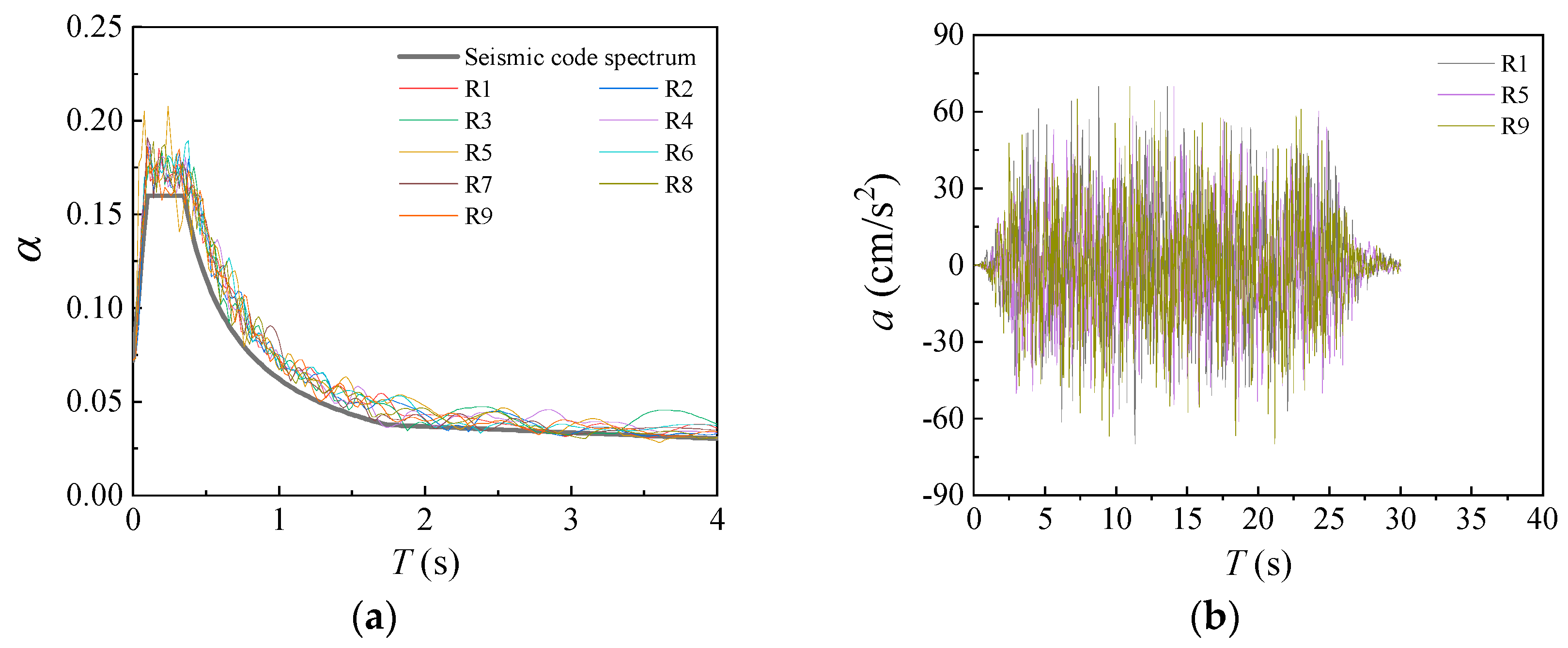
3.3. Loading Scheme

Since the dynamic response of the same structure under different earthquake actions is quite different, it is necessary to select the appropriate seismic wave to act on the structure according to the target response spectrum and relevant code [23]. The specific wave selection principles are as follows: (a) Actual strong earthquake records and artificial wave curves should be selected based on the soil condition and design seismic subgroup, with the actual number of strong earthquake records not less than 2/3 of the total number; (b) The average earthquake affecting coefficient curve of multiple time-history curves shall be statistically consistent with the seismic influence coefficient curve adopted by the response spectrum method; (c) In the elastic time-history analysis, the base shear force the structure calculated by each time-history curve shall not be less than 65% of the calculation result of the response spectrum method, and the average value of the base shear force of the structure calculated by each time-history curve shall not be less than 80% of the calculation result of the response spectrum method [23]. The natural frequency of the model is shown in

Table 4. The natural frequency of the model.

Model	Mode 1	Mode 2	Mode 3
Model-1	0.086 (X)	0.086 (Y)	0.057 (Z)
Model-2	0.127 (X)	0.127 (Y)	0.062 (Z)
Model-3	0.182 (X)	0.182 (Y)	0.086 (Z)
Model-4	0.100 (X)	0.100 (Y)	0.078 (Z)
Model-5	0.136 (X)	0.136 (Y)	0.089 (Z)
Model-6	0.189 (X)	0.189 (Y)	0.100 (Z)
Model-7	0.123 (X)	0.123 (Y)	0.101 (Z)
Model-8	0.142 (X)	0.142 (Y)	0.114 (Z)
Model-9	0.168 (X)	0.168 (Y)	0.129 (Z)

. Under the above wave selection principles, artificial waves are selected and adopted, and the corresponding time-history curve is shown in Figure 6. In addition, since the toggle brace mainly serves the frequent earthquake conditions in high-intensity areas, the peak acceleration of a seismic wave is 70 cm/s².

4. Discussion of Simulation Results

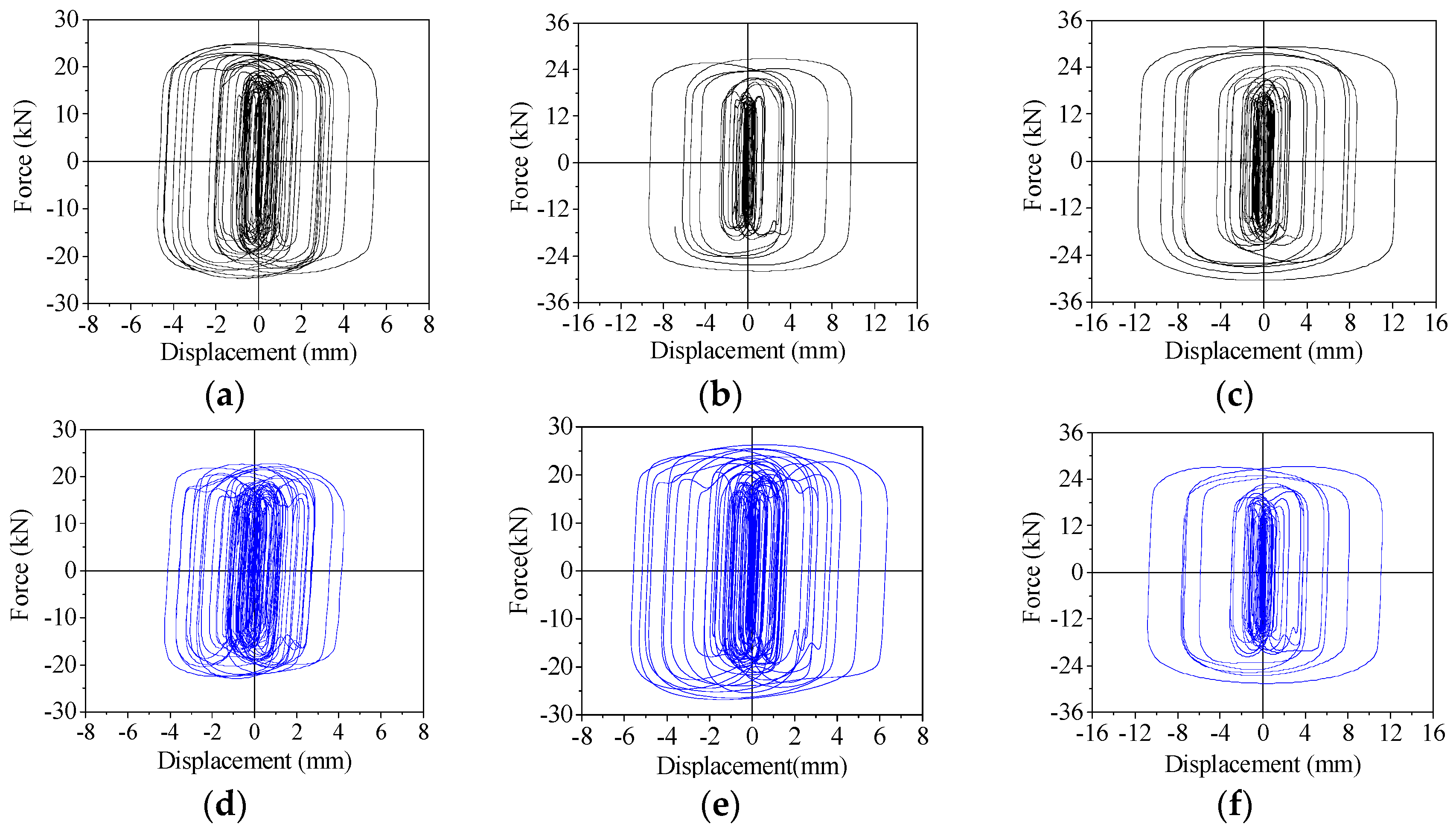
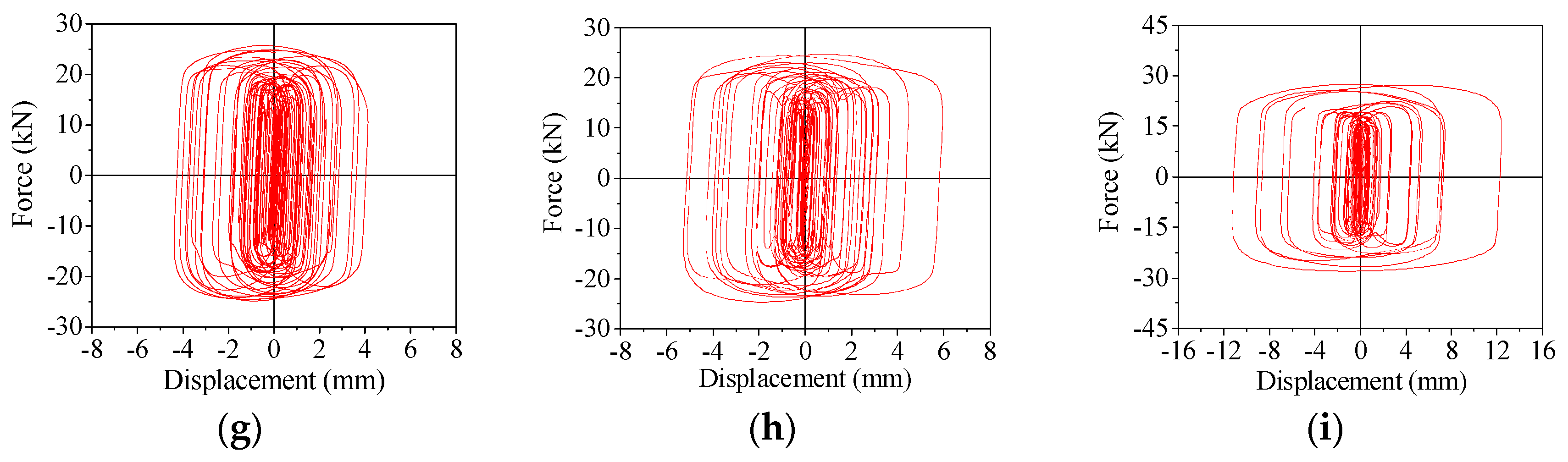
4.1. Hysteresis Curves

The hysteresis curve obtained by adjusting the angle between the viscous damper and adjacent columns to 30° is shown in Figure 7. Figure 7a–c represent the hysteresis curves of the model with a frame height of 4 m and a span of 8–12 m, respectively; Figure 7d–f represent the hysteresis curves of the model with a frame height of 5 m and a span of 8–12 m, respectively; Figure 7g–i represent the hysteresis curves of the model with a frame height of 6 m and a span of 8–12 m, respectively.

In general, similar shapes can be observed in all hysteresis curves, with hysteresis loops showing a “loop” shape. The development of the hysteresis curve has gone through a total of three stages: (a) A linear development stage, where the displacement output at both ends of the viscous damper is small, but the damper force increases significantly, and the hysteresis loop shows a linear development trend; (b) During the continuous upward stage, the hysteresis loop area significantly increases with an increase in displacement at both ends of the viscous damper; (c) During the slow descent stage, the damper force shows a decreasing trend.

Compared with Models 1–3, the output displacement of the hysteresis curve of Model 1 is only 6 mm, while the output displacements of Models 2 and 3 reach 7 mm and 9 mm, respectively. There is a significant difference in the hysteresis curve displacement of the three models, with the maximum damper forces of the three models reaching 25 kN, 30 kN, and 30 kN. The significant differences in displacement between the three models may be due to the inconsistent displacement M_f caused by the placement of viscous dampers in frames with different height-span ratios. Compared to Model 1 and Model 2, Model 3 exhibits fluctuation in the hysteresis loop, which may be due to the large span leading to some disturbance during the operation of the viscous damper.

Compared with Models 4–6, the displacement in the linear development stage of Models 4 and 5 reached 1 mm and 1.5 mm, respectively, indicating that the linear development stage is better. On the contrary, Model 6 exhibits a less significant linear development stage. The height of the frame is 5 m, and the deformation of the viscous dampers in Models 4–6 reaches 4 mm, 6 mm, and 11 mm. The corresponding maximum damper forces reach 20 kN, 25 kN, and 30 kN. In general, the greater the deformation of the viscous dampers, the more fully the damper force develops. The hysteresis curve of Model 6 exhibits certain volatility, which is basically consistent with the phenomenon presented by the hysteresis curve of Model 3, and both exist within a frame with a span of 12 m, consistent with the phenomenon mentioned above.

The hysteresis loop of Model 9 is fuller and more regular compared with the hysteresis loops of Models 7 and 8, indicating that the viscous damper has better adaptability in Model 9. Compared with Models 3 and 6, although the span of all three models is 12 m, the story height of Model 9 is higher than that of the previous two models, and the hysteresis curve does not exhibit volatility. It is speculated that this phenomenon is related to story height. The linear development stages of Model 7 and Model 8 are better than those of Model 9, implying that their linear advantages continue to decrease as story height increases. This is consistent with the phenomenon of large spans leading to certain disturbances in the working performance of viscous dampers mentioned earlier.

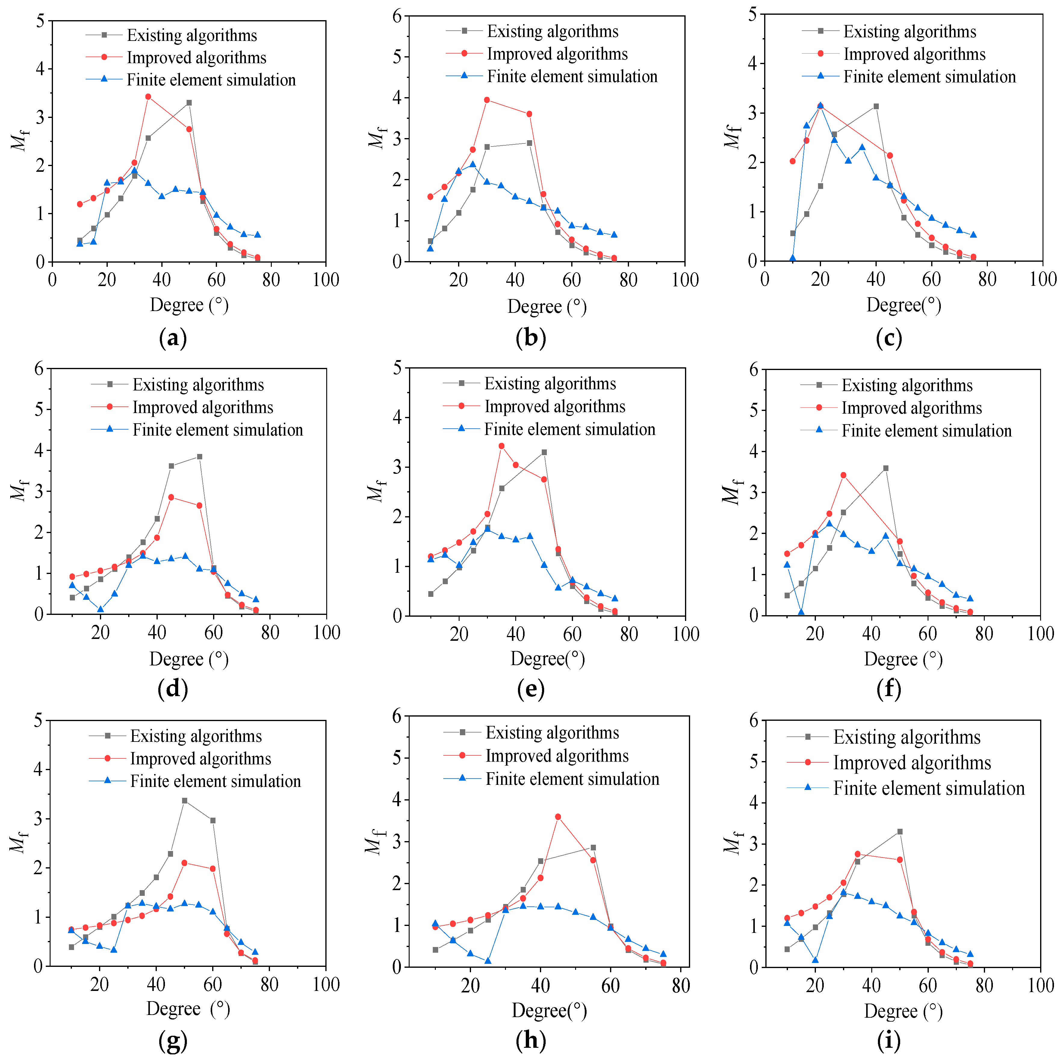
4.2. Magnification Factor

The M_f values of the viscous dampers for each model are presented in

Table 5. M_f of the different models.

Height	Span
	8 m	10 m	12 m
4 m	1.887	1.9361	2.0222
5 m	1.2179	1.7421	1.9753
6 m	1.1912	1.3484	1.8105

. Overall, the M_f values of viscous dampers are in the range of 1.1912 to 2.0222. The M_f values exhibit the following regular characteristics: (a) the M_f increases with an increase in span under an identical story height; (b) the M_f decreases with an increase in story height under the identical span, and the M_f is the highest with a story height of 4 m and a span of 12 m. M_f is the smallest for a story height of 6 m and a span of 8 m. From the above observations, it can be concluded that when the viscous damper is placed in such a “thin and high” frame, the energy dissipation of the viscous damper under earthquake action is poor due to the longer length and more vertical position of the viscous damper. However, when the viscous damper is installed in a “squat” frame with a lower story height and a larger span, the energy dissipation capacity of the viscous damper is strengthened due to its smaller length and horizontal position.

From the specific analysis results of the span-to-height ratio, it can be seen that when the span-to-height ratio is 2, the value of the M_f remains stable between 1.70 and 1.90. When the span-to-height ratio is less than 2, the M_f of all three models is less than 1.5; When the span-to-height ratio is greater than 2, the M_f of all three models is larger, and the energy dissipation ability of the viscous damper is more significant. From the above analysis, it can be seen that there is a positive correlation between the M_f and the span-to-height ratio. Therefore, it is recommended to install viscous dampers in frames with lower story heights and larger spans. This not only benefits the energy dissipation ability of viscous dampers but also reduces the probability of instability of steel frame beams, columns, and connecting components.

The M_f that can be applied to engineering usually needs to reach two, as mentioned in reference [24], but only one model mentioned above meets this standard. In order to meet the above standard, further research is needed on the M_f. The angle between the viscous damper and the column is an important factor affecting the M_f [20], so it is particularly important to explore the optimal value of the angle between the viscous damper and the column.

5. Optimization of Magnification Factor

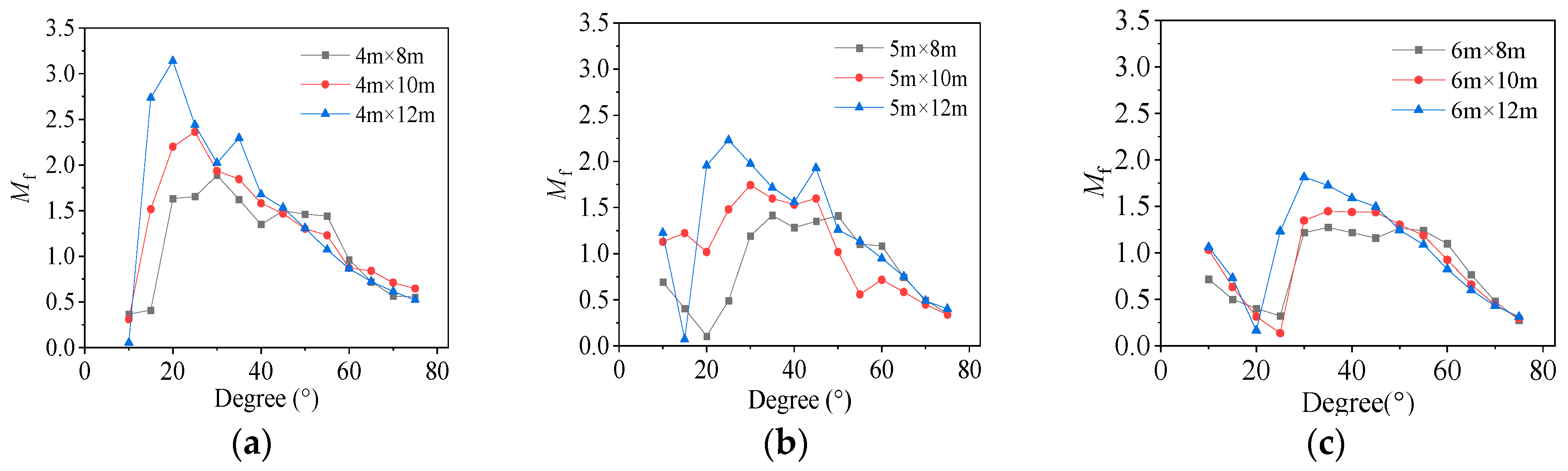
5.1. Relationship between Magnification Factor and Degree

In order to investigate the effect of different angles of viscous dampers on the M_f, numerical simulations were conducted on nine models with different angles. The M_f of each model at different angles was obtained and plotted in Figure 8. The optimal value of the M_f extracted from each model is presented in

Table 6. The optimal value of the M_f.

Height	Span
	8 m	10 m	12 m
4 m	1.8870 (30°) *	2.3630 (25°)	3.1407 (20°)
5 m	1.4147 (35°)	1.7421 (30°)	2.2291 (25°)
6 m	1.2734 (35°)	1.4484 (35°)	1.8105 (30°)

* The values in parentheses represent the degree of the viscous damper corresponding to the optimal M_f.

.

As shown in Figure 8, the variation pattern of M_f values is relatively significant, with values ranging from 0.12 to 3.14. There is a one-to-one correspondence between the angle between the viscous damper and the column and the M_f. The curve in Figure 8 shows a trend of first increasing and then decreasing, indicating that there is an optimal value for the angle between the viscous damper and the column. The angle between the viscous damper and the column is small (reference range is 10–20°), and the M_f values are all less than one. The included angle between the viscous damper and the column is moderate (reference range is 20~65°), and the M_f are all greater than one. The angle between the viscous damper and the column is relatively large (with a reference range of 65° to 80°), and the M_f are all less than one. The maximum M_f corresponding degree is within the range of 20° to 65°. The angle between the viscous damper and the column is relatively large (with a reference range of 65° to 80°), and the M_f values are all less than one. The reason for the above pattern is as follows: the upper and lower toggle-joint supports connected to the viscous damper can only generate relative angular rotation under earthquake action when the lengths of upper and lower toggle-joint supports are l₁ and l₂, respectively. The displacement generated by the viscous damper increases the amount of motion for the viscous damper, thereby increasing the energy consumption performance of the viscous damper.

As shown in Table 6, the optimal value for the M_f ranges from 1.2734 to 3.1407, and the difference in M_f values is caused by the height and span of different frames. Under an identical span, the optimal M_f value for a frame height of 4 m is greater than the optimal M_f value for a frame height of 5 m. The optimal M_f value for a frame height of 5 m is greater than the optimal M_f value for a frame height of 6 m, indicating that the larger the story height, the smaller the M_f value, and there is an inverse relationship. At an identical floor height, the optimal M_f value with a frame span of 8 m is smaller than the optimal M_f value with a frame span of 10 m. The optimal M_f value with a frame span of 10 m is smaller than the optimal M_f value with a frame span of 12 m, indicating that the value of M_f increases with an increase in the span, and this relationship is proportional. Viscous dampers are more suitable for placement in “chubby” frames, not in “tall and thin” frames. Presumably, the reason is that the viscous dampers placed on the “chubby” frame are conducive to fully exerting deformation.

For general frames with viscous dampers, the angle corresponding to the optimal M_f is usually within the range of 20° to 35°, with the number of included angles of 30° being the most significant. Therefore, when searching for the optimal M_f of each frame, the included angle of the viscous damper can be set to 30° first, and then the included angle can be verified one by one within 20°, 25°, and 35°. For frames with a span-to-height ratio of 2, the optimal M_f corresponds to an angle of 30°. For frames with a span-to-height ratio greater than 2, the angle corresponding to the M_f is less than 30°. For frames with a span-to-height ratio of less than 2, the M_f corresponds to angles greater than 30°. In addition, the optimal angle of the viscous damper decreases with an increase in span and increases with an increase in story height.

5.2. Hysteresis Curve with Optimal M_f

The hysteresis curve of the viscous damper is shown in Figure 9. All curves represent the curves corresponding to the angle between the viscous damper and the column that can achieve the optimal M_f. The story heights represented by the three hysteresis curves in each row remain consistent, and the spans represented by the three hysteresis curves in each column remain consistent.

In terms of the comparison of the hysteresis curves of the nine models, the hysteresis curves all show a “loop” shape when the viscous damper is installed in the frame. The performance of viscous dampers is relatively stable under force, which can be verified by the reduced fluctuation of the hysteresis curve. Compared with the hysteresis curve of TBVDs at a specific degree (30°), the corresponding hysteresis curve at the optimal M_f is fuller and more stable, and its energy dissipation ability is also more significant than the energy dissipation ability corresponding to the 30°. The development of the hysteresis curve has undergone three stages: a linear development stage, a stable increase stage, and a slow decrease stage. The main characteristic of the linear development stage is a significant increase in the damper force output by TBVDs at the linear development stage. During the continuous upward stage, TBVDs can maintain a relatively stable damper force as the deformation continues to increase. Models (1, 4, 7) have a span of 8 m, and their hysteresis curves exhibit a “sloping” trend due to the “thin and high” viscous dampers installed in frames with smaller spans.

The output of each type of viscous damper is maintained within the range of 20–30 kN, and the deformation of viscous dampers varies significantly within the range of 3–12 mm. The deformation of viscous dampers can be roughly divided into three intervals: 3–6 mm, 6–10 mm, and 10–12 mm. The distribution positions of the intervals coincide with the distribution intervals with span-to-height ratios less than 2, equal to 2, and greater than 2, respectively. The deformation of viscous dampers is quite significant as the span-to-height ratio of the frame gradually increases, and the corresponding energy consumption increases significantly.

6. Comparison and Analysis of Algorithms

6.1. Comparison of Algorithms

Although the calculation method for the elbow type M_f has been proposed in Chapter 1, the accuracy of the improved algorithm has not been verified. Therefore, existing algorithms and improved algorithms were used to calculate the M_f of nine models with different angles, and the results were discussed with finite element simulation. The M_f values calculated using existing algorithms, improved algorithms, and finite element simulations are plotted in Figure 10, excluding cases with high-angle sensitivity. Reference [20] points out that when the M_f of a viscous damper is greater than 4, M_f will experience significant fluctuations within a small angle range. Extract the optimal values and corresponding angles of nine model M_f values, and plot them in Figure 11a–i.

As shown in Figure 10, the relationship between the M_f values obtained from existing algorithms, improved algorithms, and finite element simulations and the angle shows a trend of first increasing and then decreasing. Starting with the comparison of the M_f values of the two algorithms and simulation results, within the range of 10–35° and 60–75°, the three calculation results are relatively consistent. However, within the range of 35–60°, the simulation results differ from the results of the two algorithms. The numerical values of the two algorithms are generally greater than the results of finite element simulation, and there is a certain error between the two algorithms and the results of finite element simulation.

As shown in Figure 11, the optimal angle and value of the M_f for both algorithms are greater than the finite element calculation results. At the same time, the optimal M_f and angle of existing algorithms are also greater than those of improved algorithms. Starting with the accuracy of the algorithm, the improved algorithm is closer to the finite element simulation results. The main reason is that the improved algorithm improves the existing algorithm by increasing the number of dependent variables, optimizing assumptions, and optimizing calculation methods, thereby making the calculation results closer to the finite element simulation. When the designer decides to install TBVDs in a specific framework during the preliminary design stage, the following two steps are necessary. Designers can first use this improved algorithm to determine the angle between the viscous damper and the column and then adjust the angle based on the results of finite element simulation. The efficiency of solving the optimal degree can be improved by using the above two steps. In summary, the improved algorithm has significant advantages in terms of accuracy and simplicity compared to existing algorithms, and the improved algorithm is more suitable for calculating the M_f values of TBVDs.

6.2. Error Analysis

There are errors in the existing algorithms, improved algorithms, and finite element simulation results. Therefore, it is necessary to analyze the sources of errors and provide ideas for improving the M_f algorithm of TBVDs. Firstly, the rigidity assumption of the toggle brace brings errors to the calculation results: when improving the algorithm to calculate the M_f, there will be imaginary solutions, which means that the upper and lower toggle braces do not intersect after the floor is laterally moved. Secondly, an infinite stiffness ratio between beams and columns can also cause errors. The upper toggle brace is connected to the middle of the frame beam, and the design concept of “strong column weak beam” inevitably considers the stiffness of the beam to be a small value. Therefore, the deformation of the beam cannot be ignored for the geometric changes of the upper and lower toggle brace. Finally, as a dynamic load, the earthquake action cannot be ignored in terms of its dynamic response to mass elements, and the same applies to the upper and lower toggle brace. The dynamic response of components is difficult to consider in static analysis and might be another important reason for algorithm errors. The calculation method of M_f under horizontal seismic action is shown in Section 2.2. However, the M_f of the TBVD of the frame under vertical seismic action cannot be calculated using this improved algorithm due to two basic assumptions: (a) the stiffness of the frame beam is infinite; (b) the changes in the elevation of the frame can be ignored. Therefore, the impact of vertical seismic action on the frame model can be ignored.

7. Conclusions

In this study, a new M_f calculation method is proposed by establishing the geometric relationship of the elbow-type viscous damper and deriving the positions of various components before and after deformation in the system. To compare the accuracy of the algorithm, finite element simulation and analysis were conducted on nine models, extracting their M_f values, and comparing their M_f values with existing and improved algorithms. The following conclusions are drawn:

• The algorithm for determining the existing M_f is relatively complex and difficult to apply in practical engineering. Considering the insufficient practicality of the existing M_f algorithm, an improved algorithm is formed based on the existing algorithm. Compared with existing algorithms, the improved algorithm optimizes assumptions and calculation methods, and its practicality has been improved.
• The correctness of the improved algorithm was verified using simulation results from nine models. From the numerical simulation results of the TBVD, it can be seen that the TBVD is relatively stable during deformation in the frame structure, and there is no fluctuation in the hysteresis loop. The hysteresis curve is relatively full, and the energy dissipation ability is significant. By comparing with simulation results, the improved algorithm outperforms existing algorithms in calculating M_f and obtaining the optimal angle.
• The M_f is related to the frame size and angle of the damper installation. Under a specific angle condition, the M_f increases with an increase in span and decreases with an increase in story height. When the installation angle range of the viscous damper is 10–20°, its M_f values are all less than 1. When the installation angle range of the viscous damper is 20–65°, the M_f values are greater than 1, and the optimal solution for the M_f is generally within this range. When the installation angle range of the viscous damper is 65–80°, the M_f values are less than 1.
• Based on the above research results, the following suggestions are proposed: designers should use the calculation method for the M_f of TBVDs proposed in this article to estimate the M_f. Designers can determine the angle corresponding to the optimal M_f roughly; TBVDs are recommended to be installed in frames with lower story heights and larger spans, where their performance is superior. The angle between the viscous damper and the frame column should be prioritized at 30 degrees and then further optimize the damping scheme.

References

- Yuan, X.; Chen, G.; Jiao, P.; Li, L.; Han, J.; Zhang, H. A Neural Network-Based Multivariate Seismic Classifier for Simultaneous Post-Earthquake Fragility Estimation and Damage Classification. Eng. Struct. 2022, 255, 113918. [Google Scholar] [CrossRef]
- Nguyen, H.D.; Lafave, J.M.; Lee, Y.J.; Shin, M. Rapid Seismic Damage-State Assessment of Steel Moment Frames Using Machine Learning. Eng. Struct. 2022, 252, 113737. [Google Scholar] [CrossRef]
- Li, H.; Xue, J.; Chen, X.; Tu, G.; Lu, X.; Zhong, R. Experimental Research on Seismic Damage of Cross-Shaped CFST Column to Steel Beam Joints. Eng. Struct. 2022, 256, 113901. [Google Scholar] [CrossRef]
- Reza Khalili, M.; Ghahremani Baghmisheh, A.; Estekanchi, H.E. Seismic Damage and Life Cycle Cost Assessment of Unanchored Brick Masonry Veneers. Eng. Struct. 2022, 260, 114187. [Google Scholar] [CrossRef]
- Li, L.; Wentao, W.; SHI, P. A Visual Data-Informed Fiber Beam-Column Model for the Analysis of Residual Hysteretic Behavior of Post-Earthquake Damaged RC Columns. J. Earthq. Eng. 2023, 1–26. [Google Scholar] [CrossRef]
- Bruschi, E.; Quaglini, V.; Calvi, P.M. A Simplified Design Procedure for Seismic Upgrade of Frame Structures Equipped with Hysteretic Dampers. Eng. Struct. 2022, 251, 113504. [Google Scholar] [CrossRef]
- Zhang, J.; Zhang, C.; Xue, Q. Insight into Energy Dissipation Behavior of a SDOF Structure Controlled by the Pounding Tuned Mass Damper System. Earthq. Eng. Struct. Dyn. 2022, 51, 958–973. [Google Scholar] [CrossRef]
- Vinayaravi, R.; Jayaraj, K.; Kumaresan, D.; Asraff, A.K. Study on Energy Dissipation Mechanism of an Impact Damper System. J. Comput. Nonlinear Dyn. 2022, 17, 041003. [Google Scholar] [CrossRef]
- Xu, Y.; Xu, Z.; Guo, Y.; Huang, X.; Dong, Y.; Li, Q. Dynamic Properties and Energy Dissipation Study of Sandwich Viscoelastic Damper Considering Temperature Influence. Buildings 2021, 11, 470. [Google Scholar] [CrossRef]
- Chen, Y.; Yu, W.; Zhang, M.; Li, Y. A Novel Energy Dissipation Damper for Multi-Level Earthquakes. J. Constr. Steel Res. 2022, 192, 107214. [Google Scholar] [CrossRef]
- Nazarimofrad, E.; Shokrgozar, A. Seismic Performance of Steel Braced Frames with Self-Centering Buckling-Restrained Brace Utilizing Superelastic Shape Memory Alloys. Struct. Des. Tall Spec. Build. 2019, 28, e1666. [Google Scholar] [CrossRef]
- Lie, W.; Wu, C.; Luo, W.; Wu, C.; Li, C.; Li, D.; Wu, C. Cyclic Behaviour of a Novel Torsional Steel-Tube Damper. J. Constr. Steel Res. 2022, 188, 107010. [Google Scholar] [CrossRef]
- Zeng, B.; Gao, J.; Qing, Y.; Wang, C.; Sun, X. Seismic Performance of Suspended-floor Structures with Viscous Dampers Considering Acceptable Interstory Drift. Struct. Des. Tall Build 2022, 31, e1912. [Google Scholar] [CrossRef]
- YupengRen; PengzhenLin; ZhigangHe Research on Application of Viscous Dampers in Continuous Steel Truss Gieder with Flexible Arch. J. Eng. Stud. 2018, 10, 546–553. [CrossRef]
- Lin, W.C.; Wang, S.J.; Hwang, J.S. Seismic Retrofit of Existing Critical Structures Using Externally Connected Viscous Dampers. Int. J. Struct. Stab. Dyn. 2022, 22. [Google Scholar] [CrossRef]
- Şigaher, A.N.; Constantinou, M.C. Scissor-Jack-Damper Energy Dissipation System. Earthq. Spectra 2003, 19, 133–158. [Google Scholar] [CrossRef]
- Hwang, J.-S.; Kim, J.; Kim, Y.-M. Rotational Inertia Dampers with Toggle Bracing for Vibration Control of a Building Structure. Eng. Struct. 2007, 29, 1201–1208. [Google Scholar] [CrossRef]
- Gluck, J.; Ribakov, Y. Active Viscous Damping System with Amplifying Braces for Control of MDOF Structures. Earthq. Eng. Struct. Dyn. 2002, 31, 1735–1751. [Google Scholar] [CrossRef]
- Berton, S.; Bolander, J.E. Amplification System for Supplemental Damping Devices in Seismic Applications. J. Struct. Eng. 2005, 131, 979–983. [Google Scholar] [CrossRef]
- Constantinou, M.C.; Tsopelas, P.; Hammel, W.; Sigaher, A.N. Toggle-Brace-Damper Seismic Energy Dissipation Systems. J. Struct. Eng. 2001, 127, 105–112. [Google Scholar] [CrossRef]
- Lee, S.-H.; Min, K.-W.; Chung, L.; Lee, S.-K.; Lee, M.-K.; Hwang, J.-S.; Choi, S.-B.; Lee, H.-G. Bracing Systems for Installation of MR Dampers in a Building Structure. J. Intell. Mater. Syst. Struct. 2007, 18, 1111–1120. [Google Scholar] [CrossRef]
- JGJ 297-2013; Technical Specification for Seismic Energy Dissipation of Buildings. China Architecture and Building Press: Beijing, China, 2012.
- GB 50011-2016; Code for Seismic Design of Buildings. China Architecture and Building Press: Beijing, China, 2016.
- Xue, J.; Luo, Z.; Sui, Y.; Yang, R.; Liu, J.; Ren, R. Seismic Mitigation Effect and Dynamic Test Study of Displacement-Amplified Viscously-Damped Outrigger. J. Build. Struct. 2022, 43, 21–31. [Google Scholar] [CrossRef]