Abstract
Bridge vortex-induced vibration (VIV) refers to the vertical resonance phenomenon that occurs in a bridge when pulsating wind passes over it and causes vortices to detach. In recent years, VIV events have been observed in numerous long-span bridges, leading to fatigue damage to the bridge structure and posing risks to driving safety. The advancement of technologies such as structural health monitoring (SHM), machine learning, and big data has opened up new research avenues for the intelligent identification of VIV in bridges. Machine learning algorithms can accurately identify the VIV events from historical data accumulated by SHM systems, thus providing an effective method for VIV recognition. Nevertheless, the existing identification methods have limitations, particularly in their applicability to bridges lacking historical VIV data. This study introduces an adaptive VIV recognition method in the main girders of long-span suspension bridges based on Transfer Component Analysis (TCA). The method can accurately identify VIV patterns in real-time or in historical data, even when specific VIV data are not available for the target bridge. The proposed method exhibits suitability for multiple long-span bridges. Experimental validation is performed using the SHM datasets from two long-span suspension bridges. The results show that the proposed VIV identification method can recognize more VIV samples compared to the benchmark model. When using sensor 1 data of bridge B as the source domain to identify the VIV of the L-section of bridge A, the F1 score of the TCA-based method is 0.836, while the F1 score of the benchmark model is 0.165. In the other 11 cases, the F1 score of the proposed model is higher than 0.8, which demonstrates the method’s robust generalization capabilities.
1. Introduction
Structural health monitoring (SHM) technology is an effective approach for studying the behavior of damage evolution in long-span bridges and plays a vital role in monitoring abnormal wind and vibration events [1,2]. An SHM system installed on a bridge can continuously collect a large amount of response data, including data during vortex-induced vibrations (VIV). These collected measurement data of VIV compensate for the limitations of wind tunnel testing and numerical simulation in the research of VIV and accurately record the VIV response of a prototype bridge in a specific wind environment, making it an important method of studying VIV. Certain SHM systems installed on long-span bridges have successfully captured data on VIV response, and researchers have conducted studies on the mechanisms of VIV occurrence in large-span bridges based on these monitoring data [3,4,5] and proposed measures to mitigate large-scale VIV [6].
Recently, SHM systems both domestically and internationally have collected extensive monitoring data on large-span bridges, including vibration data related to VIV and buffeting vibrations, as well as wind environment data [7,8,9]. To further investigate the occurrence mechanism and wind environment characteristics of VIV in bridges and study the semi-active control of VIV in bridges, it is necessary to initially develop a VIV recognition algorithm, followed by identifying the VIV data from the vast historical data and subsequently embedding the algorithm into the SHM system to enable real-time early warning of VIV, ensuring the continuous acquisition of up-to-date information on VIV. Certain researchers have suggested an unsupervised learning-based automatic extraction method for VIV employing clustering analysis. Li et al. [10] introduced a clustering analysis method to cluster the two-parameter vibration features extracted from the acceleration signals of the Xihoumen Bridge recorded between 2010 and 2014. The method also facilitates the automatic identification of the VIV component and detects VIV events with six main frequencies. Arul et al. [11] analyzed the historical data of the Burj Khalifa from 2010 to 2014 to identify VIV. They initially extracted the acceleration data features and conducted principal component analysis on them. Subsequently, clustering analysis was performed on the first two principal components, leading to the successful identification of the VIV component. Although the eddy vibration recognition algorithm based on clustering analysis has yielded relatively accurate results, manual assistance is still required to differentiate between VIV and normal vibration-induced buffeting. Moreover, cluster analysis exhibits a degree of randomness and requires the pre-specification of the number of clustering categories, leading to non-identical results in each analysis. To mitigate identification errors stemming from clustering analysis, the researchers conducted a comprehensive analysis of historical bridge monitoring data in a meticulous manner. Based on the vibration monitoring data and wind environment monitoring data, they manually comprehensively determined the time range of VIV. Finally, they established a reasonable early warning threshold, enabling the real-time identification of future VIV in the SHM system. Hua et al. [12] utilized an autoencoder to automatically extract characteristics from the acceleration sensor of the bridge’s main beam. They established a feature threshold to determine the presence of VIV. Huang et al. [13] employed the random reduction method and coefficient of variation as vibration signatures and set thresholds to automatically detect VIV data within historical data. Xu et al. [5] analyzed historical data from the Xihoumen Bridge and developed an early warning framework for VIV. The framework relies on wind parameters and vibration parameters, issuing immediate warnings when both parameters simultaneously meet the conditions for VIV. Zhao [11] investigated the monitoring data of a VIV event on a specific Yangtze River Bridge. They developed an early warning framework for VIV that enables real-time monitoring by establishing thresholds for wind parameters and vibration parameters. It is very time-consuming and labor-intensive to directly determine the VIV of historical data by using manual methods. To address this issue, Lim et al. [14] initially employed a semi-supervised method to annotate historical data. They subsequently utilized labeled datasets and deep learning methods to develop an algorithm for recognizing VIV in large-span bridges. In addition, the authors used the monitoring dataset to perform multiple trainings to determine the optimal parameter range of the recognition algorithm. It is important to note that the aforementioned methods rely on the presence of VIV samples within the bridge monitoring dataset. If the monitoring dataset of the target bridge lacks VIV samples, these methods cannot be employed to construct the VIV recognition algorithm.
The VIV of large-span bridges occurs exclusively in specific wind environments, making it challenging to gather measured VIV data for certain long-span bridges with limited service or installation time for SHM systems. Furthermore, VIV is relatively uncommon in inland areas for large-span bridges. Since the construction of the Yingwuzhou Yangtze River Bridge in 2014, there have only been two reported VIV events. In contrast, the Xihoumen Bridge, located along the coast, experiences an average of one VIV per month. Hence, the development of a VIV recognition algorithm for large-span bridges lacking historical VIV data is a crucial research topic. Kim et al. [15] proposed a VIV recognition algorithm that relies on limited vortex information. They provided a comprehensive discussion on the construction and training of the vortex recognition algorithm for two scenarios: absence of VIV data and scarcity of VIV data. When VIV data are not available, Kim [15] employs a regression model, a classification model, and an autoencoder trained on normal vibration monitoring data to assess whether the input data represent normal vibration patterns. If the input data do not correspond to normal vibration patterns, Stage 3 is utilized to ascertain whether they exhibit the characteristics of VIV. The author performed multiple training and validation experiments in the study to determine the optimal parameter range. Despite the validation of this method using the monitoring dataset of the Jindo Bridge in South Korea, it still exhibits some limitations. Firstly, the proposed network architecture is complex, requiring the construction of up to three sub-models that collaborate to create the VIV recognition algorithm. Secondly, the method still relies on the manual labeling and selection of the monitoring dataset for the target bridge, guided by expert knowledge. Moreover, it necessitates individual establishment and training for each specific bridge.
Traditional machine learning is built upon the assumption of “independent and identically distributed” data, which posits that the training and test data are independently sampled from the same distribution [16,17]. Under this assumption, the generalization error of a machine learning model tends to decrease as the size of the training set increases. As an example, the well-known iris dataset comprises 150 records with four characteristics: sepal length, sepal width, petal length, and petal width. These features are used to determine the category of iris flowers. The training and test sets are constructed in a way that preserves the same feature distributions as the original iris dataset. This ensures that a machine learning algorithm trained on this dataset can effectively identify the type of iris. However, in certain specific tasks, the data distribution may differ [18]. For instance, as depicted in Figure 1, handwritten digit recognition models are often trained on the MNIST handwriting dataset. However, real-world handwritten digit images are not limited to black characters on a white background; they can have various background colors, as seen in the MNIST-M dataset. Applying a number recognition algorithm trained solely on the MNIST dataset to the MNIST-M dataset would yield suboptimal recognition results.
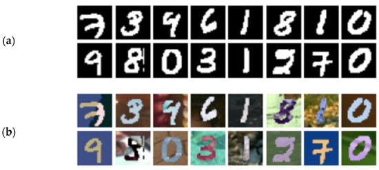
Figure 1.
(a) MNIST handwriting dataset; (b) MNIST-M mixed background handwritten dataset [18].
Transfer learning is employed to address this issue by leveraging a pre-trained model to tackle a new, analogous task [19], thereby enhancing task performance. In conjunction with the principles of transfer learning, the domain from which knowledge, data, and labels are transferred or previously learned is referred to as the source domain, while the domain to be learned is known as the target domain. For instance, in the aforementioned example, the MNIST dataset serves as the source domain, while the MNIST-M dataset represents the target domain. Transfer learning technology revolves around the observation that data in the source and target domains are distributed according to disparate distributions. Consequently, machine learning algorithms trained on the source domain exhibit strong performance on the target domain.
This study is motivated by the transfer learning method and presents an adaptive VIV recognition method for long-span suspension bridge based on Transfer Component Analysis (TCA). The method utilizes a bridge dataset with VIV monitoring data as the source domain, and identifies VIV of the target bridge in real-time or in historical datasets even without VIV data of the target bridge, and it is also applicable to multiple long-span bridges. The proposed method is validated using the SHM dataset from two long-span suspension bridges, demonstrating its strong generalization capability.
2. Methodology
2.1. TCA
Transfer Component Analysis (TCA) was initially proposed in 2011 by Yang from the Hong Kong University of Science and Technology [20]. TCA is a method of transferring feature transformations that maps both the source and target domains into a new feature space, where a classifier can be used in the source domain and the target domain is constructed. Before delving into the detailed theory, let us establish the following definitions: the source domain is , the source domain label is , where and are the source domain samples and their corresponding labels, and is the number of source domain samples; the target domain is , and the target domain has samples and no labels. TCA begins by assuming the existence of a mapping function that transfers the source domain and the target domain into a new feature space. This mapping aims to ensure a similar edge distribution distance between the source and target domains within the space , thereby achieving approximate equality in the conditional distribution of both domains . Subsequently, a classification algorithm is trained in the new feature space and then applied to the target domain.
The main objective of TCA is to discover an optimal mapping that minimizes the “distance” between the source and target domains in the new feature space. Numerous methods exist to quantify the “distance” between data samples from distinct distributions, including the KL (Kullback–Leibler) divergence. However, these methods often necessitate the introduction of additional parameters or intermediate density estimations. In TCA, the authors employed an unparameterized distance metric called the maximum mean discrepancy (MMD) [21] to gauge the separation between the source and target domains in the Reproducing Kernel Hilbert Space (RKHS), as demonstrated in Equation (1). Here, denotes the norm within the RKHS.
Generally, the function exhibits strong nonlinearity, and direct optimization using the aforementioned equation may cause to fall into a poor local optimal solution. TCA, on the other hand, employs the kernel function in place of . Consequently, the objective becomes solving the kernel matrix . Once the source and target domains are mapped with the kernel matrix , the MMD can be represented by Equation (2):
Here,
In the equation mentioned above, the term “trace” represents the sum of the diagonal elements of a matrix. With the problem now reduced to minimizing Equation (2) by solving a kernel matrix, one approach to tackle this problem is through the use of semi-definite programming (SDP). However, employing SDP can be computationally intensive and resource-consuming, making it impractical for large datasets. To address this limitation, TCA has introduced additional enhancements. TCA decomposes the kernel matrix into and introduces , resulting in a reduction of the kernel matrix to a dimensional space. This space includes .
Among these, and . In the MMD distance metric formula, TCA employs as a replacement for the kernel matrix by substituting Equation (5) into Equation (2) to obtain Equation (6). By introducing , the final distance measurement formula demonstrates a reduction in the dimensionality of the kernel matrix, thereby simplifying the calculation process.
Apart from minimizing the distance between the source and target domains, TCA’s final optimization goal also encompasses two additional considerations. First, it aims to control the complexity of by introducing a regularization term, , into the optimization objective. Second, TCA emphasizes not only reducing the distance between and but also maximizing the preservation of useful features in the target domain through the mapping . This ensures the retention of data differences during target domain learning. The above equation reveals that the projection of the source or target domain sample in the embedded hidden space is represented as . Here, column i denotes the embedding coordinate of . Consequently, the divergence of the projection sample is determined as . In this context, corresponds to the central matrix, represents a column vector with all elements set to 1, and signifies the identity matrix of . In order to maximize the preservation of data differences for optimization objectives, we set . To summarize, the final optimization objectives of unsupervised TCA are as follows:
The parameter serves as a trade-off that regulates the complexity of . By leveraging techniques like Lagrangian duality, TCA ultimately computes the combination of -order eigenvectors with as . The aforementioned process represents the solution approach of unsupervised TCA, which operates without employing source domain labels, thereby qualifying it as an unsupervised learning method. However, in scenarios where source domain data are labeled, TCA also introduces a corresponding solution called SSTCA (semi-supervised TCA) to leverage as much known label information as possible. Interested readers can refer to the paper in [20] for further details. In summary, whether it is unsupervised TCA or semi-supervised SSTCA, both methods are straightforward to use, and the pseudocode for TCA is presented in Algorithm 1.
| Algorithm 1: TCA |
| Input: Source domain data , source domain label , target domain data |
Output:
|
2.2. Feature Extraction
Prior to constructing the recognition algorithm, it is important to identify the distinct bridge vortex features from the buffeting. While deep-learning-based classification algorithms commonly employ deep neural networks as feature extractors for signals or images, the vibration characteristics of the bridge during vortex-induced vibration significantly differ from those observed during normal buffeting. These differences include the presence of large vortex acceleration amplitudes and the concentration of vibration energy at specific frequencies. Hence, the vortex-induced vibration classification algorithm does not require neural networks for feature extraction; instead, it can leverage existing physical laws to construct sensitivity features specific to VIV.
Based on previous related studies, the ten-minute-long acceleration signal was utilized to extract six vibration signatures, encompassing both statistical and frequency domain characteristics. The statistical characteristics consist of the root mean square amplitude of acceleration , variance V, and Hopkins statistic H. Notably, during vortex-induced vibration, the acceleration amplitude surpasses that observed during normal jitter, demonstrating prominent periodic changes. The root mean square amplitude serves as an effective indicator of acceleration data amplitude variations, while the variance signifies the periodic changes in the data. The Hopkins statistic, commonly employed to assess data clustering tendencies, reveals a distinct clustering trend in vortex-induced vibration acceleration data, unlike the normal jitter period [11].
In the equation above, represents the number of signal sampling points, represents the acceleration or deflection data, and denotes the average of the vibration signal. The calculation of Equation (9) is intricate. Firstly, a set of points is randomly selected from the points of the data sample. Then, for each in the sample space, the closest point is determined, and the minimum distance, denoted as , is obtained to form the distance vector . Subsequently, points are randomly generated within the possible value range of the sample, and for each generated point , the nearest sample point in the sample space is identified. The minimum distance is calculated, resulting in the distance vector . Finally, the Hopkins statistic is computed according to Equation (9).
To capture the distinct spectral characteristics of VIV and buffeting vibration, the following two frequency domain characteristics are primarily extracted: the main frequency PSD amplitude P and the energy concentration coefficient R. Figure 2 provides a visual representation of P and R, wherein the energy concentration coefficient R is the ratio of the main frequency PSD amplitude P to the second main frequency PSD amplitude. Furthermore, VIV exhibits a phenomenon known as frequency locking, whereby the bridge’s significant vibration influences the shedding frequency of the vortex. As a result, changes in wind speed within a certain range do not alter the frequency of the bridge’s VIV. This section introduces a novel characteristic index, namely the main frequency change value . It is computed by dividing the ten-minute acceleration data segment into two five-minute segments and calculating the difference between the main frequency of the first five minutes of data and the main frequency of the last five minutes of data.
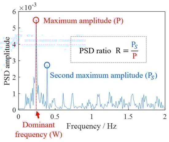
Figure 2.
Definition of frequency domain characteristics.
2.3. Algorithm Framework
This section presents an adaptive method for identifying VIV in the main girders of long-span suspension bridges based on TCA. The proposed method is applicable to identifying VIV data in different long-span bridges without the need for historical data. AIA-VIV can be applied directly to the target bridge monitoring dataset or historical extensive monitoring data for identifying vortex-excited vibrations. Figure 3 illustrates a schematic diagram of the AIA-VIV algorithm, comprising three main components. The first part involves dataset acquisition and feature extraction. The target bridge dataset is utilized as the target domain data, which do not include labels, while the source domain data comprise labeled vibration data from other bridge datasets. The second part pertains to transfer learning, where various unsupervised transfer learning methods discussed in Section 2.1 are employed to align feature samples across domains. The target domain remains unchanged, while the source domain becomes an adapted source domain. The third part focuses on the classifier. The trained SVM classifier can perform real-time recognition of vortex-induced vibrations in target bridges and also identify VIV data in large historical datasets.
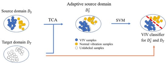
Figure 3.
Algorithm framework.
3. Datasets
3.1. Bridge A
Bridge A is a long-span suspension bridge spanning the Yangtze River and connecting Hanyang and Wuchang in Wuhan. It has three towers and a four-span steel-girder concrete deck. The bridge is equipped with 58 sensors, including thermometers, anemometers, inclinometers, displacement meters, and accelerometers. Figure 4 depicts the sensor arrangement employed in this study. A hydro-static, positioned from segments B to X, is utilized to measure the vertical deflection of the main beam. The longitudinal accelerometer is mounted atop the central tower, while the transverse and vertical accelerometers for the main beam are positioned at the bottom center of sections I, K, L, and Q. Additionally, the main cable accommodates transverse and vertical accelerometers. The HMS utilizes an accelerometer sensor with a sampling frequency of 20 Hz, while all other sensor types operate at a sampling rate of 0.25 Hz. For detailed information about Bridge A and its structural health monitoring (SHM) system, refer to article [22].
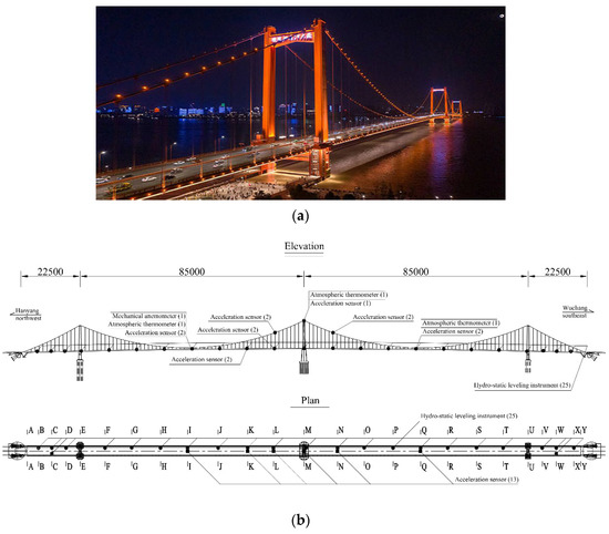
Figure 4.
Bridge A. (a) The real bridge overview, (b) layout diagram of monitoring sensors in section A of the bridge (unit: cm).
The dataset for Bridge A consists of monitoring data collected on a specific day in April 2020, encompassing measurements such as displacement, acceleration, wind speed, and wind direction. Figure 5 displays the vertical acceleration monitoring data for the Q section and I section on that day. The Q section represents the middle span of the main span in the Wuchang direction, while the I section corresponds to the middle position of the main span in the Hanyang direction. The figure clearly indicates a complete absence of acceleration data after 17:00, suggesting a possible failure of Bridge A’s accelerometer signal collector at that time. Analysis of the Q-section data reveals an abrupt increase in acceleration amplitude starting at 12:00, lasting approximately one hour, with a peak amplitude of 580 mm/s2. This event signifies the occurrence of the first abnormal vibration. Subsequently, the acceleration reverts to its normal amplitude. However, at 16:10, there is a sudden increase in acceleration. Due to the missing data after 17:00, it is not possible to determine the maximum amplitude precisely. Nonetheless, based on the observed data, the maximum amplitude has surpassed that of the first abnormal vibration, nearly reaching 590 mm/s2, marking the occurrence of the second abnormal vibration. Notably, during the abnormal vibration, the acceleration amplitude of the I segment exhibits a slight increase. However, the maximum amplitude of the I segment falls below the warning threshold specified in the standard, and it is considerably smaller than the acceleration amplitude observed in the Q section. Consequently, the analysis leads to the conclusion that the acceleration amplitude characteristics of the main span in the Wuchang direction are prominently evident, whereas the acceleration amplitude characteristics of the main span in the Hanyang direction are less pronounced.
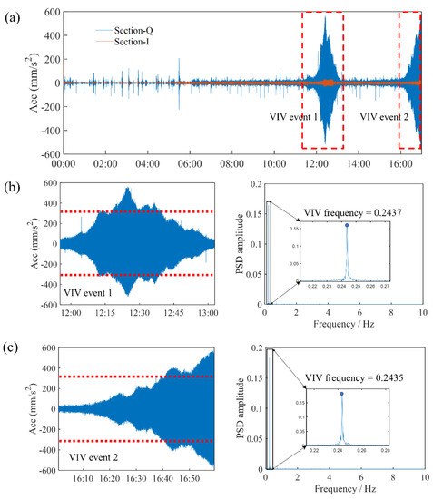
Figure 5.
The accelerometer data for Bridge A, including (a) vertical accelerometer data for the Q section and I section; (b) the first VIV data of the Q section along with its PSD diagram; (c) the data of the second VIV of the Q section and its corresponding PSD diagram. According to Chinese regulations, the red dashed line represents the first level warning value of VIV with a root mean square (rms) acceleration of 315 mm/s2.
The PSD diagram in Figure 5 reveals that the two main frequencies associated with the abnormal vibrations, 0.2437 Hz and 0.2435 Hz, are extremely close. Moreover, the vibration magnitude of the second main frequency is insignificant compared to that of the first main frequency, which is aligned with the characteristics of self-excited vibrations. Furthermore, the occurrence of sudden amplitude increases on multiple occasions corroborates the conclusion that the abnormal vibration event is induced by VIV.
3.2. Bridge B
Bridge B, a two-span asymmetrical steel box girder suspension bridge with a total length of 2713 m, spans the East China Sea and connects two islands. Its main span measures 1650 m, ranking third globally. The north and south towers of the suspension bridge are 236.5 m high prestressed concrete structures. In 2020, the bridge’s operation and maintenance department upgraded and maintained the health monitoring system. The new system, depicted in Figure 6, was designed based on the analysis of previous bridge monitoring data and vibration characteristics. It features a simplified sensor layout compared to the old system. The number of main beam vibration sensors was reduced to three, positioned at 3/8 span, 1/2 span, and 5/8 span. Additionally, one acceleration sensor per span was placed on the downstream guardrail position of the bridge, operating at a sampling frequency of 50 Hz. Wind speed monitoring is facilitated by a single anemometer located at the center of the main span, also with a sampling frequency of 50 Hz.
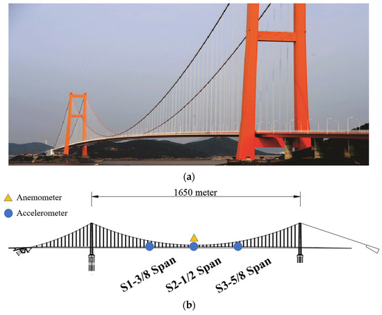
Figure 6.
Bridge B. (a) The real bridge overview, (b) the sensor layout of the new health monitoring system.
The monitoring dataset for Bridge B in January 2021 includes data from three accelerometers as well as wind speed and direction sensors. Artificial analysis was conducted to identify both VIV and normal vibration data. Furthermore, the wind environment and vibration monitoring data during the VIV event were briefly analyzed. Figure 7 illustrates the identified abnormal monitoring data from Bridge B in January.
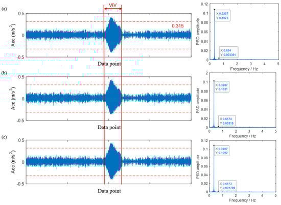
Figure 7.
The data on VIV events and the magnitude map of Power Spectral Density (PSD) for Bridge B in January. The data include the sensor readings and PSD amplitude maps for (a) B1, (b) B2, and (c) B3 sensors.
The significant anomalous vibration event started at 11:09 p.m. on January 23 and lasted approximately three hours, concluding around 1:50 a.m. on January 24. Analysis of the three acceleration data PSD diagrams during this time period reveals that the primary frequency of bridge vibration is 0.3287 Hz, with the vibration mode occupying an overwhelmingly dominant position. The PSD amplitude at this frequency is approximately 0.1. The second main frequency is 0.654 Hz, with a significantly lower PSD amplitude of only about 0.002. Consequently, the energy concentration coefficient during this vibration event is well below 0.1. Given the large acceleration amplitude and these findings, the abnormal vibrations can be considered as VIV.
4. Verification
In this section, we apply the VIV identification method based on the TCA algorithm to analyze its advantages in a VIV identification task. The proposed algorithm utilizes the monitoring dataset from Bridge B as the source domain and applies it to Bridge A to identify VIV events specific to Bridge A. Suppose our objective is to develop a VIV identification algorithm for Bridge A, which lacks historical VIV data. In this case, we can employ the monitoring dataset of Bridge A as the target domain and the monitoring dataset of Bridge B as the source domain within the VIV identification method based on the TCA algorithm. Bridge B is equipped with three acceleration sensors, and the feature sample sets extracted from its dataset can serve as the source domain. On the other hand, Bridge A comprises two sensors, and the feature sample sets extracted from its dataset can be utilized as the target domain. It is important to note that the VIV algorithm is constructed independently for each sensor’s monitoring data.
To assess the advantages of the proposed method algorithm over conventional algorithms, four metrics are employed: accuracy, recall, precision, and F1 score, which play a crucial role in evaluating the quality of VIV recognition results (see Figure 8). Each of these metrics is measured on a scale from 0 to 1, where a higher value signifies a superior algorithm model.
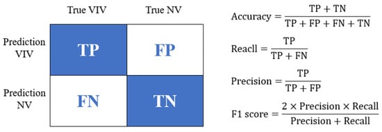
Figure 8.
Definition of evaluation indicators for the evaluation of VIV tasks.
The algorithm used in this case involves identifying the B1 dataset as the source domain and the AL dataset as the target domain. The results obtained from this analysis are presented in Table 1. The “noDA” algorithm refers to a VIV recognition algorithm that is directly trained on the source data and applied to the target dataset without employing any transfer learning methods. From Table 1, it can be observed that the noDA algorithm manages to identify a little number of VIV data instances. This can be attributed to the fact that VIV is a self-excited resonance phenomenon, and the vibration characteristics exhibited by different large-span bridges during VIV are similar. The six extracted vibration characteristics exhibit consistent trends, such as increasing root mean square acceleration values and decreasing capacity concentration factors. Consequently, this algorithm is selected as the baseline model for the recognition task. To further enhance the VIV identification process, the subsequent step involves utilizing the TCA algorithm. The outcomes of this approach are also presented in Table 1, highlighting the improved accuracy, recall, precision, and F1 score in comparison to the noDA benchmark model.

Table 1.
B1 as the source domain and the results of VIV identification in AL.
Figure 9 further supports this observation, as it shows that the TCA algorithm identifies more VIV data compared to the noDA algorithm. The thicker bars in the graph represent the VIV data identified by the TCA algorithm. Additionally, Figure 10 provides a visual comparison of the VIV data identified by both the noDA and TCA algorithms. The blue part of the graph shows the manually identified VIV data, and the red part shows the algorithm-identified VIV data. The graph shows that the TCA algorithm accurately identifies the formation and dissipation of VIV, and it identifies more VIV data compared to the noDA algorithm. Based on the analysis of the B1-AL condition, it can be concluded that the TCA algorithm performs better than the noDA algorithm in identifying VIV data.
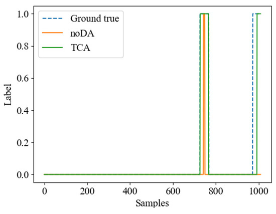
Figure 9.
noDA vs. TCA VIV identification results.
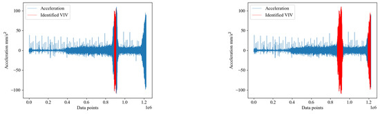
Figure 10.
B1 dataset for VIV data in source domain identification AL (noDA on the left, TCA on the right).
To further validate the advantage of the TCA-based algorithm over the noDA algorithm, additional experiments were conducted to identify VIV data in different bridge datasets. The VIV data were identified using B1, B2, and B3 as the source domain and AQ and AL as the target domain, and the results are shown in Table 2. Table 2 shows the results of these experiments, which indicate an improvement in accuracy, recall, precision, and F1 score compared to the results of the noDA algorithm.
Table 2.
Bridge B as source domain; Bridge A VIV identification results.
The proposed method in this paper aims to identify VIV data within bridge datasets by utilizing a specific bridge dataset that includes both VIV data and manually delineated VIV labels as the source domain. To demonstrate the effectiveness of the VIV identification method based on the TCA algorithm across different scenarios, we evaluate its performance using the bridge A monitoring dataset as the source domain and the bridge B monitoring dataset as the target domain. From the data in Table 3, it can be observed that the TCA algorithm outperforms the noDA algorithm in all four metrics (accuracy, recall, precision, and F1 score), and the F1 scores are closer to one.
Table 3.
Bridge A as source domain; Bridge B VIV identification results.
Based on the above analysis, it can be concluded that the TCA algorithm achieves superior results compared to the benchmark model (no transfer learning algorithm is used, and the VIV classifier is directly trained on the source domain and applied to the target bridge) in both scenarios where Bridge A is used as the source domain to identify vortex samples in Bridge B and vice versa.
5. Conclusions
This paper introduces an adaptive recognition method for vortex-induced vibration (VIV) in long-span suspension bridges using the Transfer Component Analysis (TCA) technique. The proposed method addresses the limitations of traditional algorithms, such as difficulties in obtaining VIV data, applicability to only a single bridge, and reliance on manual judgment. It enables real-time or historical dataset analysis to identify the VIV of the long-span bridges, even if the target bridge has no or limited VIV data. To verify the effectiveness of the proposed method, monitoring data from Bridge A and Bridge B were utilized. The proposed algorithm based on TCA consistently outperforms the benchmark model, regardless of whether it identifies the VIV in Bridge B using Bridge A as the source domain or identifies the VIV in Bridge A using Bridge B as the source domain. Unlike the benchmark model, which solely trains the VIV classifier on the source domain and applies it directly to the target bridge, the proposed method incorporates transfer learning algorithms and achieves better identification results. However, the method proposed in this paper still has the potential to improve the accuracy of VIV recognition, and researchers can try to use different domain adaptive methods to achieve better VIV recognition results in the future.
Author Contributions
Conceptualization, S.C.; Methodology, J.H. and S.C.; Software, P.L.; Validation, H.H. and C.W.; Formal analysis, Z.Z.; Investigation, H.H. and Z.Z.; Data curation, S.C., H.H. and Z.Z.; Writing—original draft, J.H.; Writing—review & editing, C.W., P.L. and Y.L.; Visualization, M.N.; Supervision, C.W. and M.N.; Project administration, Y.L.; Funding acquisition, C.W. All authors have read and agreed to the published version of the manuscript.
Funding
This research received no external funding.
Data Availability Statement
The data that support the findings of this study are available from the corresponding author upon reasonable request.
Acknowledgments
This work was supported by the National Key R&D Program of China (2021YFE0112200), Open Fund of Research and Development Center of Transport Industry of New Generation of Artificial Intelligence Technology, the Japan Society for Promotion of Science (Kakenhi No. 18K04438), the Tohoku Institute of Technology research Grant, and the National Natural Science Foundation of China (Grant No. 52178115).
Conflicts of Interest
The authors declare no conflict of interest.
References
- VAnnamdas, G.M.; Bhalla, S.; Soh, C.K. Applications of structural health monitoring technology in Asia. Struct. Health Monit.-Int. J. 2017, 16, 324–346. [Google Scholar] [CrossRef]
- Comisu, C.-C.; Taranu, N.; Boaca, G.; Scutaru, M.-C. Structural health monitoring system of bridges. Procedia Eng. 2017, 199, 2054–2059. [Google Scholar] [CrossRef]
- Cantero, D.; Oiseth, O.; Ronnquist, A. Time-Frequency Analysis of Suspension Bridge Response for Identification of Vortex Induced Vibrations. In Proceedings of the International Conference on Experimental Vibration Analysis for Civil Engineering Structures (EVACES), Univ California San Diego, San Diego, CA, USA, 12–14 July 2017; pp. 667–675. [Google Scholar]
- Cantero, D.; Oiseth, O.; Ronnquist, A. Indirect monitoring of vortex-induced vibration of suspension bridge hangers. Struct. Health Monit.-Int. J. 2018, 17, 837–849. [Google Scholar] [CrossRef]
- Xu, S.Q.; Ma, R.J.; Wang, D.L.; Chen, A.R.; Tian, H. Prediction analysis of vortex-induced vibration of long-span suspension bridge based on monitoring data. J. Wind Eng. Ind. Aerodyn. 2019, 191, 312–324. [Google Scholar] [CrossRef]
- Zhao, L.; Cui, W.; Shen, X.M.; Xu, S.Y.; Ding, Y.J.; Ge, Y.J. A fast on-site measure-analyze-suppress response to control vortex-induced-vibration of a long-span bridge. Structures 2022, 35, 192–201. [Google Scholar] [CrossRef]
- Abdeljaber, O.; Avci, O.; Kiranyaz, M.S.; Boashash, B.; Sodano, H.; Inman, D.J. 1-D CNNs for structural damage detection: Verification on a structural health monitoring benchmark data. Neurocomputing 2018, 275, 1308–1317. [Google Scholar] [CrossRef]
- Bao, Y.Q.; Li, H. Machine learning paradigm for structural health monitoring. Struct. Health Monit.-Int. J. 2021, 20, 1353–1372. [Google Scholar] [CrossRef]
- Cawley, P. Structural health monitoring: Closing the gap between research and industrial deployment. Struct. Health Monit.-Int. J. 2018, 17, 1225–1244. [Google Scholar] [CrossRef]
- Li, S.; Laima, S.; Li, H. Cluster analysis of winds and wind-induced vibrations on a long-span bridge based on long-term field monitoring data. Eng. Struct. 2017, 138, 245–259. [Google Scholar] [CrossRef]
- Arul, M.; Kareem, A.; Kwon, D.K. Identification of Vortex-Induced Vibration of Tall Building Pinnacle Using Cluster Analysis for Fatigue Evaluation: Application to Burj Khalifa. J. Struct. Eng. 2020, 146, 04020234. [Google Scholar] [CrossRef]
- Hua, X.; Sun, R.; Wen, Q.; Chen, Z.; Yan, Y. Automatic detection of vortex-induced resonance events in bridges using novelty detection. J. Vib. Eng. 2018, 31, 948–956. [Google Scholar]
- Huang, Z.W.; Li, Y.Z.; Hua, X.G.; Chen, Z.Q.; Wen, Q. Automatic Identification of Bridge Vortex-Induced Vibration Using Random Decrement Method. Appl. Sci. 2019, 9, 2049. [Google Scholar] [CrossRef]
- Lim, J.; Kim, S.; Kim, H.-K. Using supervised learning techniques to automatically classify vortex-induced vibration in long-span bridges. J. Wind Eng. Ind. Aerodyn. 2022, 221, 104904. [Google Scholar] [CrossRef]
- Kim, S.; Kim, T. Machine-learning-based prediction of vortex-induced vibration in long-span bridges using limited information. Eng. Struct. 2022, 266, 114551. [Google Scholar] [CrossRef]
- Choi, R.Y.; Coyner, A.S.; Kalpathy-Cramer, J.; Chiang, M.F.; Campbell, J.P. Introduction to Machine Learning, Neural Networks, and Deep Learning. Transl. Vis. Sci. Technol. 2020, 9, 14. [Google Scholar] [PubMed]
- Janiesch, C.; Zschech, P.; Heinrich, K. Machine learning and deep learning. Electron. Mark. 2021, 31, 685–695. [Google Scholar] [CrossRef]
- Zhuang, F.Z.; Qi, Z.Y.; Duan, K.Y.; Xi, D.B.; Zhu, Y.C.; Zhu, H.S.; Xiong, H.; He, Q. A Comprehensive Survey on Transfer Learning. Proc. IEEE 2021, 109, 43–76. [Google Scholar] [CrossRef]
- Lu, J.; Behbood, V.; Hao, P.; Zuo, H.; Xue, S.; Zhang, G. Transfer learning using computational intelligence: A survey. Knowl.-Based Syst. 2015, 80, 14–23. [Google Scholar] [CrossRef]
- Pan, S.J.; Tsang, I.W.; Kwok, J.T.; Yang, Q.A. Domain Adaptation via Transfer Component Analysis. In Proceedings of the 21st International Joint Conference on Artificial Intelligence (IJCAI-09), Pasadena, CA, USA, 11–17 July 2009; pp. 1187–1192. [Google Scholar]
- Bernhard, S.; John, P.; Thomas, H. A Kernel Method for the Two-Sample-Problem. In Advances in Neural Information Processing Systems 19: Proceedings of the 2006 Conference; MIT Press: Cambridge, MA, USA, 2007; pp. 513–520. [Google Scholar]
- Zhao, H.W.; Ding, Y.L.; Li, A.Q.; Liu, X.W.; Chen, B.; Lu, J. Evaluation and Early Warning of Vortex-Induced Vibration of Existed Long-Span Suspension Bridge Using Multisource Monitoring Data. J. Perform. Constr. Facil. 2021, 35, 04021007. [Google Scholar] [CrossRef]


Disclaimer/Publisher’s Note: The statements, opinions and data contained in all publications are solely those of the individual author(s) and contributor(s) and not of MDPI and/or the editor(s). MDPI and/or the editor(s) disclaim responsibility for any injury to people or property resulting from any ideas, methods, instructions or products referred to in the content. |
© 2023 by the authors. Licensee MDPI, Basel, Switzerland. This article is an open access article distributed under the terms and conditions of the Creative Commons Attribution (CC BY) license (https://creativecommons.org/licenses/by/4.0/).