Enhancing the Seismic Performance of Adjacent Building Structures Based on TVMD and NSAD

Abstract

Under the action of an earthquake, the adjacent building structure will have a large displacement and even cause damage to the structure. Structure displacement can be suppressed by adding a tuned viscous mass damper (TVMD) and negative stiffness amplifier damper (NSAD) between adjacent structures. This paper deduces the motion equation of adjacent building structures under earthquake action. The transfer function of the vibration control system is obtained using Laplace transform. The parameter optimization analysis of the structural vibration control system is carried out through $H_2$ norm theory. The vibration control performance of the TVMD vibration control system and NSAD vibration control system is studied by taking two adjacent building structures composed of single freedom building structures as an example. The results show that the two vibration damping devices proposed in this paper can play the role of vibration control. The influence of the same parameters on the two structures is not completely consistent. Under seismic excitation, the NSAD control system has better displacement control ability than the TVMD control system.

1. Introduction

When adjacent structures are influenced by earthquake excitation, different structural failures are caused by various reasons [1,2]. For example, near-faulted earthquakes cause greater displacement and velocity, which increases the force caused by the impact and leads to greater damage [3]. In addition, the influence of adjacent structures in an earthquake is gradually increasing every year, and it is inevitable to consider the interaction between adjacent structures and the impact of collapse on the surrounding buildings [4]. A common response is to form a structural vibration control device [5,6,7,8,9,10,11,12,13,14,15,16] through different combinations of dampers, spring stiffness and other additional devices, including additional mass blocks, inertial vessels and negative stiffness. The adjacent structures have been investigated and analyzed in terms of vibration control through the connection control method [17]. The motion equations of two adjacent multi-degree-of-freedom (MODF) structures are effectively derived [18]. When studying adjacent buildings, an anti-seismic structure vibration control strategy was proposed [19]. In this paper, the damping effects of a TVMD control system consisting of damper, spring stiffness and additional mass block and an NSAD control system consisting of damper, spring stiffness and negative stiffness in adjacent structures will be studied. In recent years, scholars have conducted much research on the vibration reduction of adjacent structures. In this research, the additive mass or inertial mass is used as the vibration control device. Therefore, the innovation of this paper is to apply a negative stiffness damper (NSD) to the vibration control of adjacent buildings and compare it with a TVMD vibration control system. In addition, the $H_2$ norm theory is combined with the Monte Carlo algorithm, and the optimal values of the parameters are obtained by MATLAB numerical simulation.

Passive control technology has the advantages of a simple structure, low cost, stable performance and no additional energy input [20]. In the past few decades, passive control technology has been widely studied and applied in the field of structural vibration reduction [21]. In the past decade, two different passive control technologies have received increasing attention, including negative stiffness control (NS). Negative stiffness has been used in a variety of practical engineering fields [22,23,24,25,26,27,28,29,30,31,32,33,34,35,36,37,38,39,40,41,42,43,44], including vehicle construction, bridge construction, damper devices and various seismic strategies. Negative stiffness can reduce the response to vibration, ensuring the use of precision instruments in high-frequency vibration [45]. The negative stiffness device and isolation strategy can work together to decrease structural displacement and the acceleration response [46]. The improved adaptive negative stiffness device can also effectively reduce the seismic response of the structure [47]. Compared with traditional damping devices, passive negative stiffness devices have better vibration control effects [48]. In addition, damping devices with negative stiffness elements have a better energy dissipation capacity than traditional damping devices [49]. Wang et al. [50] improved the energy dissipation capacity of the damper by taking advantage of inertial vessels and negative stiffness. In addition, Wang et al. [43,51] proposed a negative stiffness amplification damper, which can achieve a significant damping amplification effect. Negative stiffness devices and dampers have effective control effects on both elastic and inelastic systems [52,53]. The inherent feature of NSAD is that the energy dissipation effect is significantly enhanced, but it lacks a complete energy dissipation theory. The obvious difference between the energy dissipation enhancement technique of negative stiffness and the deformation amplification mechanism based on lever has not been studied or discussed [54].

This paper constructs two kinds of adjacent building structure vibration control systems, mainly studying the vibration control ability of two kinds of vibration control systems in earthquake excitation. First, the motion equations of two vibration control systems are derived. The transfer function of the system is calculated by Laplace transform. The parameters of the NSAD vibration control system are optimized by $H_2$ norm theory and the optimal solution is obtained. Finally, the effect of negative stiffness on vibration reduction of adjacent structures is revealed by numerical analysis and time history analysis, and the effect is compared with that of the TVMD vibration control system.

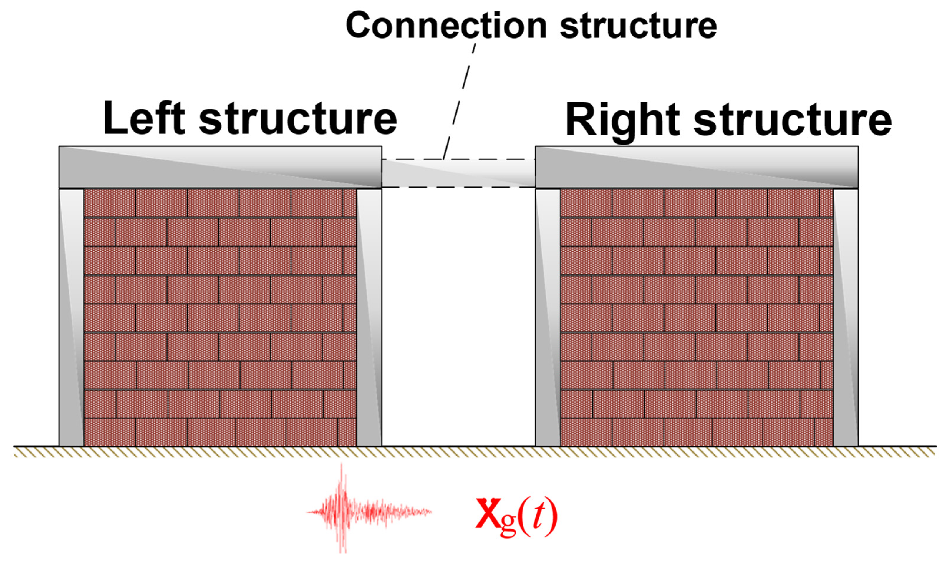
2. Vibration Control System of Adjacent Structures Based on TVMD/NSAD

Two single-story adjacent structure building models are shown in Figure 1. In order to facilitate calculation and analysis, the architectural model is simplified, as shown in Figure 2. This section will achieve the effect of vibration reduction through the appropriate combination of stiffness spring, viscous damper, mass block and negative stiffness element. As shown in Figure 2, additional mass and additional negative stiffness are used to achieve vibration reduction. In TVMD control systems and NSAD control systems, the inertial mass $m_d$ and NSD will amplify the motion of the viscous damper. Due to the presence of the connecting spring $k_d$, the amplified deformation is absorbed by spring deformation. Therefore, the total deformation of the additional device is not magnified. The structure of the TVMD control system is shown in Figure 2. The TVMD control system is configured by connecting the inertial mass $m_d$ and the viscous damper $c_d$ in parallel, supporting the combination of the two frames with the horizontal stiffness of $k_d$. Similarly, replacing the inertial mass $m_d$ with the negative stiffness $k_N$ will enable the configuration of the NSAD control system (see Figure 2).

As a vibration damping device, the calculation analysis of the TVMD control system and NSAD control system will be affected by the inertial mass $m_d$ and NSD $k_N$. This will be discussed in detail in Section 3.

The motion equations of the TVMD vibration control system and NSAD vibration control system are presented.

$${\mathit{M}}_{TVMD}{\ddot{\mathit{X}}}_{TVMD}+{\mathit{C}}_{TVMD}{\dot{\mathit{X}}}_{TVMD}+{\mathit{K}}_{TVMD}{\mathit{X}}_{TVMD}+f_d=-{\mathit{M}}_{TVMD}{\mathsf{\Gamma }}_{TVMD}{\ddot{x}}_g$$

(1)

$${\mathit{M}}_{NSAD}{\ddot{\mathit{X}}}_{NSAD}+{\mathit{C}}_{NSAD}{\dot{\mathit{X}}}_{NSAD}+{\mathit{K}}_{NSAD}{\mathit{X}}_{NSAD}+f_d=-{\mathit{M}}_{NSAD}{\mathsf{\Gamma }}_{NSAD}{\ddot{x}}_g$$

(2)

for TVMD vibration control systems,

$$f_d=f_{\mathrm{T}\mathrm{V}\mathrm{M}\mathrm{D}}=m_d{\ddot{x}}_d+c_d{\dot{x}}_d=k_d(x_l-x_d)$$

(3)

for NSAD vibration control systems,

$$f_d=f_{\mathrm{N}\mathrm{S}\mathrm{A}\mathrm{D}}=k_N{x}_d+c_d{\dot{x}}_d=k_d(x_l-x_d)$$

(4)

Thus, we get the matrix equation.

TVMD vibration control system,

$$\left[\begin{array}{ccc}{m}_l& 0& 0\\ 0& m_r& m_d\\ 0& 0& m_d\end{array}\right]\left[\begin{array}{c}{\ddot{x}}_l\\ {\ddot{x}}_r\\ {\ddot{x}}_d\end{array}\right]+\left[\begin{array}{ccc}{c}_l& 0& 0\\ 0& c_r& c_d\\ 0& 0& c_d\end{array}\right]\left[\begin{array}{c}{\dot{x}}_l\\ {\dot{x}}_r\\ {\dot{x}}_d\end{array}\right]+\left[\begin{array}{ccc}{k}_l+k_d& 0& {-k}_d\\ 0& k_r& 0\\ {-k}_d& 0& k_d\end{array}\right]\left[\begin{array}{c}{x}_l\\ x_r\\ x_d\end{array}\right]=-\left[\begin{array}{ccc}{m}_l& 0& 0\\ 0& m_r& m_d\\ 0& 0& m_d\end{array}\right]\left[\begin{array}{ccc}1& 0& 0\\ 0& 1& 0\\ 0& 0& 0\end{array}\right]{\ddot{x}}_g$$

(5)

NSAD vibration control system,

$$\left[\begin{array}{ccc}{m}_l& 0& 0\\ 0& m_r& 0\\ 0& 0& 0\end{array}\right]\left[\begin{array}{c}{\ddot{x}}_l\\ {\ddot{x}}_r\\ {\ddot{x}}_d\end{array}\right]+\left[\begin{array}{ccc}{c}_l& 0& 0\\ 0& c_r& c_d\\ 0& 0& c_d\end{array}\right]\left[\begin{array}{c}{\dot{x}}_l\\ {\dot{x}}_r\\ {\dot{x}}_d\end{array}\right]+\left[\begin{array}{ccc}{k}_l+k_d& 0& {-k}_d\\ 0& k_r& k_N\\ {-k}_d& 0& k_d\end{array}\right]\left[\begin{array}{c}{x}_l\\ x_r\\ x_d\end{array}\right]=-\left[\begin{array}{ccc}{m}_l& 0& 0\\ 0& m_r& 0\\ 0& 0& 0\end{array}\right]\left[\begin{array}{ccc}1& 0& 0\\ 0& 1& 0\\ 0& 0& 0\end{array}\right]{\ddot{x}}_g$$

(6)

where $m_d$ is the mass in the attached device; $c_d$ is the damping coefficient of the viscous damper; $k_d$ is the stiffness of the connecting spring in the adjacent structural model; $k_N$ is the negative stiffness provided by NSD in the NSAD control system; $x_d$ is the deformation displacement of the viscous damper, and also the deformation displacement of inertial mass $m_d$ in TVMD vibration control system and $k_N$ in NSAD control system.

In this paper, the transfer function of the motion equation can be obtained by the ratio of the structural response to the Laplace transform of the external excitation.

$$\mathit{H}\left(\lambda \right)=\frac{\mathit{M}\mathsf{\Gamma }}{-\mathit{M}{\omega }^2+\mathit{C}j\omega +\mathit{K}}=\left[\begin{array}{c}{H}^l\left(\lambda \right)\\ H^r\left(\lambda \right)\end{array}\right]$$

(7)

where the superscript “l” and the superscript “r” represent the “left structure” and “right structure”, respectively.

$${\mathit{H}}_{TVMD/NSAD}\left(\lambda \right)=\frac{{\mathit{M}}_{TVMD/NSAD}{\mathsf{\Gamma }}_{TVMD/NSAD}}{-{\mathit{M}}_{TVMD/NSAD}{\omega }^2+{\mathit{C}}_{TVMD/NSAD}j\omega +{\mathit{K}}_{TVMD/NSAD}}=\left[\begin{array}{c}{H}^l\left(\lambda \right)\\ H^r\left(\lambda \right)\\ H_{TVMD/NSAD}\left(\lambda \right)\end{array}\right]$$

(8)

where the subscript “TVMD/NSAD” represents the motion equation of $m_d$/$k_N$ in the TVMD/NSAD vibration control system.

3. Vibration Transfer Function of Adjacent Building Structures Based on TVMD and NSAD

3.1. Calculation of Transfer Function

Frequency domain analysis is a classical method to study control systems. In this section, we will use the transfer function to reveal the damping effect of the TVMD control system and NSAD control system. This section will focus on the maximum value of the transfer function in Equation (9),

$$J_{TVMD/NSAD}^{l/r}={max}_{\lambda }\left\{{\mathit{H}}_{TVMD/NSAD}^{l/r}\left(\lambda \right)\right\}$$

(9)

where $\lambda =\frac{\omega }{{\omega }_l}$; $\omega$ is the external seismic excitation frequency; ${\mathit{H}}^{l/r}\left(\lambda \right)$ is the amplitude of the transfer function of the “left structure” and “right structure” in the adjacent building structure, respectively. ${\mathit{H}}_{TVMD/NSAD}^{l/r}\left(\lambda \right)$ is the transfer function of the “left structure” and “right structure” in the two vibration control systems, respectively.

Therefore, in order to obtain a concrete expression of the transfer function in Equation (9), the following dimensionless parameters will be introduced.

$${\mathsf{\omega }}_l=\sqrt{\frac{k_l}{m_l}}, {\mathsf{\omega }}_r=\sqrt{\frac{k_r}{m_r}}, {\mathsf{\xi }}_l=\frac{c_l}{2\sqrt{k_l{m}_l}}, {\mathsf{\xi }}_r=\frac{c_r}{2\sqrt{k_r{m}_r}}, f=\frac{{\mathsf{\omega }}_r}{{\mathsf{\omega }}_l}$$

(10)

The following dimensionless parameters are introduced:, ${\xi }_d=\frac{c_d}{2\sqrt{k_d{m}_d}}$, ${\mu }_1=\frac{m_d}{{\mathrm{m}}_{\mathrm{l}}}$, ${\mu }_2=\frac{m_d}{m_r}$, $f_1=\frac{{\mathsf{\omega }}_r}{{\mathsf{\omega }}_l}$ ($f$ and $f_1$ express the same parameter information; the difference is that $f_1$ is to distinguish the parameter symbols under the two structural systems); $f_2=\frac{{\mathsf{\omega }}_d}{{\mathsf{\omega }}_l}$ (The ratio of the frequency ratio of the damping device to the frequency ratio of the “left structure”).

The transfer function of the TVMD vibration control system can be obtained.

$$H_{TVMD}^l\left(i\lambda \right)=\frac{{\lambda }^2{A}_2^l+\lambda A_1^l+A_0^l}{{\lambda }^4{B}_4^l+{\lambda }^3{B}_3^l+{\lambda }^2{B}_2^l+\lambda B_1^l+B_0^l}$$

(11)

where

• $A_0^l=-f_2^2$
• $A_1^l=-2\mathrm{i}{f}_2{\xi }_d$
• $A_2^l=1$
• $B_0^l=f_2^4{\mu }_1+f_2^2(1+f_2^2{\mu }_1)$
• $B_1^l=2\mathrm{i}{f}_2^2{\xi }_l+2\mathrm{i}{f}_2(1+f_2^2{\mu }_1){\xi }_d$
• $B_2^l=-f_2^2+(-1-f_2^2{\mu }_1)-4f_2{\xi }_l{\xi }_d$
• $B_3^l=-2\mathrm{i}{\xi }_l-2\mathrm{i}{f}_2{\xi }_d$
• $B_4^l=1$
• $B_3=0$

$$H_{TVMD}^r\left(i\lambda \right)=\frac{{\lambda }^4{A}_4^r+{\lambda }^3{A}_3^r+{\lambda }^2{A}_2^r+\lambda A_1^r+A_0^r}{{\lambda }^6{B}_6^r+{\lambda }^5{B}_5^r+{\lambda }^4{B}_4^r+{\lambda }^3{B}_3^r+{\lambda }^2{B}_2^r+\lambda B_1^r+B_0^r}$$

(12)

where

• $A_0^r=f_1^2{f}_2^2(1+2f_2^2{\mu }_1)$
• $A_1^r=2\mathrm{i}{f}_1^2{f}_2({\xi }_d+f_2({\xi }_l+f_2({\mu }_1-{\mu }_2){\xi }_d\left)\right)$
• $A_2^r=f_1^2(-1-f_2^2(1+{\mu }_1-{\mu }_2)-4f_2{\xi }_l{\xi }_d)$
• $A_3^r=-2\mathrm{i}{f}_1^2({\xi }_l+f_2{\xi }_d)$
• $A_4^r=f_1^2$
• $B_0^r=-f_1^2{f}_2^2(1+2f_2^2{\mu }_1)$
• $B_1^r=-2\mathrm{i}{f}_1{f}_2^2(1+2f_2^2{\mu }_1){\xi }_r-2\mathrm{i}{f}_1^2{f}_2({\xi }_d+f_2({\xi }_l+f_2{\mu }_1{\xi }_d\left)\right)$
• $B_2^r=f_2^2(1+2f_2^2{\mu }_1)+f_1^2(1+f_2^2(1+{\mu }_1)+4f_2{\xi }_l{\xi }_d)+4f_1{f}_2{\xi }_r({\xi }_d+f_2({\xi }_l+f_2{\mu }_1{\xi }_d\left)\right)$
• $B_3^r=2\mathrm{i}{f}_1^2({\xi }_l+f_2{\xi }_d)+2\mathrm{i}{f}_1{\xi }_r(1+f_2^2(1+{\mu }_1)+4f_2{\xi }_l{\xi }_d)+2\mathrm{i}{f}_2({\xi }_d+f_2({\xi }_l+f_2{\mu }_1{\xi }_d\left)\right)$
• $B_4^r=-f_1^2-4f_1{\xi }_r({\xi }_l+f_2{\xi }_d)+(-1-f_2^2(1+{\mu }_1)-4f_2{\xi }_l{\xi }_d)$
• $B_5^r=-2\mathrm{i}{f}_1{\xi }_r-2\mathrm{i}({\xi }_l+f_2{\xi }_d)$
• $B_6^r=$1

The following parameters are introduced: $\mu =\frac{m_l}{m_r}$ (The ratio of the “left structure” mass to the “right structure” mass); $\eta =\frac{k_N}{k_l}$ (negative stiffness ratio); $\theta =\frac{k_d}{k_l}$ (additional stiffness ratio); $\phi =\frac{c_d}{c_l}$ (additional damping ratio); and $f=\frac{{\mathsf{\omega }}_r}{{\mathsf{\omega }}_l}$ (the ratio of the “left structure” frequency ratio to the “right structure” frequency ratio). The transfer function of the NSAD control system can be obtained.

$$H_{NSAD}^l\left(i\lambda \right)=\frac{\lambda D_1^l+D_0^l}{{\lambda }^3{E}_3^l+{\lambda }^2{E}_2^l+\lambda E_1^l+E_0^l}$$

(13)

where

• $D_0^l=-(\eta +\theta )$
• $D_1^l=-2\mathrm{i}\phi {\xi }_l$
• $E_0^l=\eta +\theta +\eta \theta$
• $E_1^l=2\mathrm{i}(\eta +\theta +\phi +\theta \phi ){\xi }_l$
• $E_2^l=-\eta -\theta -4\phi {\xi }_l^2$
• $E_3^l=-2\mathrm{i}\phi {\xi }_l$

$$H_{NSAD}^l\left(i\lambda \right)=\frac{{\lambda }^3{D}_3^r+{\lambda }^2{D}_2^r+\lambda D_1^r+D_0^r}{{\lambda }^5{E}_5^r+{\lambda }^4{E}_4^r+{\lambda }^3{E}_3^r+{\lambda }^2{E}_2^r+\lambda E_1^r+E_0^r}$$

(14)

where

• $D_0^r=f^2(-\theta +\eta (-1+(-1+\mu )\theta \left)\right)$
• $D_1^r=-2\mathrm{i}{f}^2(\eta +\phi +\theta (1+\phi -\mu \phi \left)\right){\xi }_l$
• $D_2^r=f^2(\eta +\theta +4\phi {\xi }_l^2)$
• $D_3^r=2\mathrm{i}{f}^2\phi {\xi }_l$
• $E_0^r=f^2(\eta +\theta +\eta \theta )$
• $E_1^r=2\mathrm{i}{f}^2(\eta +\theta +\phi +\theta \phi ){\xi }_l+2\mathrm{i}f(\eta +\theta +\eta \theta ){\xi }_r$
• $E_2^r=(-\eta -\theta -\eta \theta )-f^2(\eta +\theta +4\phi {\xi }_l^2)-4f(\eta +\theta +\phi +\theta \phi ){\xi }_l{\xi }_r$
• $E_3^r=-2\mathrm{i}{f}^2\phi {\xi }_l-2\mathrm{i}(\eta +\theta +\phi +\theta \phi ){\xi }_l-2\mathrm{i}f(\eta +\theta +4\phi {\xi }_l^2){\xi }_r$
• $E_4^r=(\eta +\theta +4\phi {\xi }_l^2)+4f\phi {\xi }_l{\xi }_r$
• $E_5^r=2\mathrm{i}\phi {\xi }_l+f^2(\eta +\theta +\eta \theta )$

For the above TVMD vibration control system and NSAD vibration control system, this paper will follow the usual methods used in the literature. It is assumed that one part of the parameters is known, and the other part of the parameters are used as the target design parameters. After the objective parameters and objective functions are determined, parameter analysis is carried out.

3.2. Parameter Analysis

In this section, the transfer function of the system is analyzed by assuming parameter conditions. This section assumes that the damping ratio ${\xi }_l$ of the “left structure”, damping ratio ${\xi }_r$ of the “right structure” and frequency ratio $f$($f_1$) in the TVMD vibration control system and NSAD vibration control system are the same as the parameter conditions of adjacent building structures without control.

3.2.1. $H_{TVMD}^{l/r} \left(\lambda \right)$

For the TVMD vibration control system. In this section, the parameters (frequency ratio $f_2$ and mass ratio ${\mu }_1$) contained in Equations (11) and (12) are compared and analyzed.

Figure 3 plots the transfer function images of the “left structure” and the “right structure” in the TVMD vibration control system with respect to parameter $f_2$. Figure 3a is the transfer function image of the “left structure” in the TVMD vibration control system. Figure 3a draws 10 transfer function curves with different values of parameter $f_2$ based on parameter assumptions. For different value intervals of parameter $f_2$, the curve details of the three intervals are enlarged in Figure 3a. The blue text in the figure shows the value range of parameter $f_2$. The direction of the blue arrow shows the law of increasing and decreasing the peak value of the transfer function curve at a certain interval of parameter $f_2$. The peak value of the transfer function curve decreases with the linear increase in parameter $f_2$ in the interval ${0.1\le f}_2\le 0.4$. When $f_2=0.1$, the peak value of the transfer function curve reaches the maximum in the interval, and the amplitude at the peak is 5.04. In the interval ${0.5\le f}_2\le 0.8$, the peak value of the transfer function curve increases with the linear increase of $f_2$. In the interval ${0.9\le f}_2\le 1$, the peak value of the transfer function curve gradually decreases with the linear increase of the parameter $f_2$. In general, the peak value of the transfer function curve of the left structure at the interval ${0.1\le f}_2\le 1$ shows a law of decreasing first, increasing and then decreasing. It can be seen from Figure 4a that the peak value of the thick black solid line representing the uncontrolled structure system is much larger than the peak value of the transfer function in the vibration control system. The vibration of the “left structure” is effectively controlled.

Figure 3b shows the transfer function image of the “right structure” in the TVMD vibration control system. In the figure, it can be clearly observed that the transfer function of the “right structure” has obvious double peaks. Additionally, parameter $f_2$ is divided into three interval segments. In the interval ${0.1\le f}_2\le 0.4$, the peak value of the transfer function also decreases with the linear increase of $f_2$. With the linear increase of parameter $f_2$ in the interval ${0.5\le f}_2\le 0.8$, the amplitudes at both peaks of the transfer function begin to increase. In the interval ${0.9\le f}_2\le 1$, with the linear increase of parameter $f_2$, the amplitude at the double crest of the transfer function decreases continuously. The law of the transfer function of the “right structure” with respect to the parameter $f_2$ is the same as that of the “left structure”. In Figure 4b, the amplitude of the transfer function of the uncontrolled system is also larger than that of the control system.

Figure 5 draws the transfer function images of “left structure” and “right structure” in the TVMD vibration control system with respect to parameter ${\mu }_1$. In Figure 5a, as the mass ratio ${\mu }_1$ increases linearly, the peak value of the transfer function decreases approximately linearly. Similarly, in Figure 6a, the amplitude of the transfer function of the “left structure” in the TVMD vibration control system is effectively reduced, and the vibration is effectively controlled.

In Figure 5b, with the linear increase of the mass ratio ${\mu }_1$, the amplitude of the transfer function of the “right structure” tends to increase. It can be observed from the enlarged figure in Figure 5b that the larger the value of parameter ${\mu }_1$, the smaller the increase of the amplitude of the transfer function.. Then, compared with the “right structure” of the original building, it can be observed from Figure 6b that the vibration of the “right structure” is effectively controlled.

Figure 7a draws a three-dimensional graph of the “left structure” with respect to parameters $f_2$ and $\lambda$. It can be seen from the curve in Figure 7a that the law of increase and decrease of the peak value of the two-dimensional curve of parameter $f_2$ is consistent with the law summarized in Figure 3a. Moreover, the peak value of the transfer function reaches its maximum value when $f_2=0.8$. The transfer function of the “left structure” in the TVMD vibration control system is significantly reduced compared with the “left structure” in the non-control system. Figure 7b draws a three-dimensional graph of the “right structure” with respect to the parameters “right structure” and $\lambda$. When $f_2=0.4$ or so, the peak value of the transfer function has an obvious trough. The vibration of the “right structure” is controlled to the greatest extent. When $f_2\ge 0.5$, the transfer function begins to show obvious double peaks. The transfer function of the “right structure” in the TVMD vibration control system is significantly reduced compared with the right structure in the non-control system. It can be observed in Figure 8a that the peak value of the transfer function curve continues to decrease with a small amplitude. It can also be observed from Figure 8b that when ${\mu }_1<5$, the peak growth rate of the transfer function is faster, and when ${\mu }_1>5$, the peak growth rate of the transfer function begins to slow down.

In this section, parameters $f_2$ and ${\mu }_1$ are analyzed. The linear increase of parameter $f_2$ makes the transfer function curves of “left structure” and “right structure” increase and decrease in the same way. The amplitude of the structure transfer function is reduced effectively compared with the original structure. The linear increase in the parameter ${\mu }_1$ makes the transfer function curves of the “left structure” and the “right structure” present two opposite increasing and decreasing rules, respectively. However, in the TVMD vibration control system, the amplitude of the structure transfer function is also effectively reduced.

3.2.2. $H_{NSAD}^{l/r} \left(\lambda \right)$

The NSAD vibration control system is analyzed in this section. For the NSAD vibration control system, this section will compare and analyze the parameters (negative stiffness ratio $\eta$; additional stiffness ratio $\theta$ and additional damping ratio $\phi$).

Figure 9 plots the transfer function of the “left structure” and the “right structure” with respect to the negative stiffness ratio $\eta$ in the NSAD vibration control system. It is found that the negative stiffness ratio $\eta$ can be divided into $\eta >-0.5$ and $\eta <-0.5$. Figure 9a, b plots the transfer function image of the “left structure” in the NSAD vibration control system. See Figure 9a. With the negative stiffness decreasing compared with $\eta$, the peak value of the transfer function of the “left structure” decreases first and then increases. The peak value of the transfer function reaches its minimum value when $\eta =-0.25$. This can be observed in Figure 9b. When $\eta <-0.5$, the peak value of the transfer function decreases continuously. The smaller the negative stiffness is than $\eta$, the smaller the reduction in the peak value of the transfer function. In Figure 10a,b, it can be observed that the peak value of the transfer function of the “left structure” is effectively reduced under the control system.

Figure 9c,d plots the transfer function image of the “right structure” in the NSAD vibration control system. See Figure 9c. When $0<\eta <-0.4$, the peak value of the transfer function increases gradually. When $-0.4<\eta <-0.5$, the peak value of the transfer function decreases gradually. This can be observed in Figure 9d. The amplitude of the transfer function decreases gradually when $\eta <-0.5$. The smaller the negative stiffness is than $\eta$, the smaller the transfer function peak decline. It can be observed in Figure 10c,d that under the control system, the peak value of the transfer function of the “right structure” is also effectively reduced.

Figure 11 plots the transfer function of the “left structure” and the “right structure” with respect to the additional stiffness ratio $\theta$ in the NSAD vibration control system. Figure 11a shows the transfer function image of the “left structure” in the NSAD vibration control system. When $\theta \le 0.6$, the peak value of the transfer function gradually decreases, and when $\theta >0.6$, the transfer function gradually increases. The “left structure” in the NSAD vibration control system in Figure 12a is compared with the “left structure” in the original uncontrolled system. The peak value of the transfer function is effectively reduced.

Figure 11b shows the transfer function image of the “right structure” in the NSAD vibration control system. For the “right structure”, the parameter $\theta$ is also discussed in two intervals. The peak value of transfer function to decreases gradually when $\theta \le 0.6$. When $\theta >0.6$, the transfer function begins to increase gradually. In Figure 12b, the peak value of the transfer function of the “right structure” in the NSAD vibration control system is also effectively reduced compared with the “right structure” in the original uncontrolled system.

Figure 13 plots the transfer function of the “left structure” and the “right structure” with respect to the additional damping ratio $\phi$ in the NSAD vibration control system. Figure 13a shows the transfer function image of the “left structure” in the NSAD vibration control system. It can be observed from the marked peak of the curve in the enlarged figure that the change in the additional damping ratio $\phi$ has little effect on the transfer function. The peak value of the transfer function also decreases as the additional damping ratio $\phi$ increases linearly. In combination with Figure 13a, it can be seen that the peak value of the three-dimensional curve gradually decreases. The peak value of the transfer function is also reduced in Figure 14a.

Figure 13b shows the transfer function image of the “right structure” in the NSAD vibration control system. It can be observed from the marked peak of the curve in the enlarged figure that the change in the additional damping ratio $\phi$ also has little effect on the transfer function of the “right structure”. However, the difference is that as the additional damping ratio $\phi$ increases linearly, the peak value of the transfer function begins to increase gradually Figure 14b also shows that the amplitude of the transfer function is reduced.

This can be observed in Figure 15a, a three-dimensional graph of the negative stiffness ratio $\eta$. The peak value of the transfer function increases sharply at $\eta =-0.5$, and only part of the image is captured in order to clearly observe the curve. The overall trend of the peak value of the transfer function increases gradually when $\eta >-0.5$ and decreases gradually when $\eta <-0.5$. The left structure in the NSAD vibration control system is compared with the “left structure” in the original uncontrolled system. This can be observed in Figure 15b, a three-dimensional graph of the negative stiffness ratio $\eta$. The curve of parameter $\eta$ is consistent with the curve of the transfer function of the “left structure”. The overall trend of the peak value of the transfer function increases gradually when $\eta >-0.5$ and decreases gradually when $\eta <-0.5$. The “right structure” in the NSAD vibration control system is compared with the “right structure” in the original uncontrolled system. In Figure 16a, it can also be observed that when $\theta \le 0.6$, obvious wave peaks appear in the three-dimensional graph and the peaks gradually decrease. When $\theta =0.6$, the three-dimensional graph has a clear trough and the amplitude at the crest increases gradually when $\theta >0.6$. In Figure 16b, the peaks and troughs of the “right structure” with respect to parameter $\theta$ are more obvious. When $\theta \le 0.6$, the wave crest appears obvious, and the peak value decreases gradually. There is a clear trough at $\theta =0.6$ and the amplitude at the crest increases gradually when $\theta >0.6$. It can be observed from the three-dimensional curve in Figure 17a that there is no obvious fluctuation in the three-dimensional curve. In Figure 17b, it can be observed that the peak value of the three-dimensional curve with respect to the additional damping ratio $\phi$ increases by a small amplitude.

In summary, the NSAD vibration control system can also effectively reduce the amplitude of the transfer function of adjacent building structures. The transfer function images of the “left structure” and the “right structure” have even function properties at a negative stiffness ratio $\phi =-0.5$. The transfer function images of “left structure” and “right structure” have opposite increasing and decreasing rules on both sides of the additional stiffness ratio $\theta =0.6$. The additional damping ratio $\phi$ has little effect on the transfer function of the “left structure” and the “right structure”. The increase of the additional damping ratio $\phi$ makes the peak value of the “left structure” transfer function decrease slowly, and the peak value of the “right structure” transfer function to increase slowly.

4. Optimization of Vibration Parameters of Adjacent Building Structures Based on ${\mathit{H}}_2$ Norm Theory and the Monte Carlo Mode Search Method

In this section, the parameters of the vibration control system of adjacent building structures are optimized by using $H_2$ norm theory. The main purpose of this paper is to avoid the collision between adjacent buildings, so this section regards the “left structure” and the “right structure” as a whole. The relative displacement ($X_l-X_r$) between the “left structure” and the “right structure” is analyzed. When the relative displacement between buildings is reduced, the possibility of collisions between adjacent buildings can be effectively reduced. Lists the transfer function about the relative displacement between the “left structure” and the “right structure”,

$$H_{TVMD}\left(i\lambda \right)=\frac{X_l-X_r}{{\ddot{x}}_g/{\omega }_l^2}=\frac{{\lambda }^3{A}_3+{\lambda }^2{A}_2+\lambda A_1+A_0}{{\lambda }^6{B}_6+{\lambda }^5{B}_5+{\lambda }^4{B}_4+{\lambda }^3{B}_3+{\lambda }^2{B}_2+\lambda B_1+B_0}$$

(15)

where

• $A_0=f_2^2(-1+f_1^2-2f_2^2{\mu }_1)$
• $A_1=-2\mathrm{i}{f}_2\left(f_2\right({\xi }_l-f_1{\xi }_r)-(-1+f_1^2+f_2^2(-{\mu }_1+{\mu }_2)\left){\xi }_d\right)$
• $A_2=1-f_1^2-f_2^2(-{\mu }_1+{\mu }_2)+4f_2{\xi }_l{\xi }_d-4f_1{f}_2{\xi }_r{\xi }_d$
• $A_3=2\mathrm{i}({\xi }_l-f_1{\xi }_r)$
• $B_0=-f_1^2{f}_2^2(1+2f_2^2{\mu }_1)$
• $B_1=-2\mathrm{i}{f}_1{f}_2^2(1+2f_2^2{\mu }_1){\xi }_r-2\mathrm{i}{f}_1^2{f}_2({\xi }_d+f_2({\xi }_l+c{\mu }_1{\xi }_d\left)\right)$
• $B_2=f_2^2(1+2f_2^2{\mu }_1)+f_1^2(1+f_2^2(1+{\mu }_1)+4f_2{\xi }_l{\xi }_d)+4f_1{f}_2{\xi }_r({\xi }_d+f_2({\xi }_l+f_2{\mu }_1{\xi }_d\left)\right)$
• $B_3=2\mathrm{i}{f}_1^2({\xi }_l+f_2{\xi }_d)+2\mathrm{i}{f}_1{\xi }_r(1+f_2^2(1+{\mu }_1)+4f_2{\xi }_l{\xi }_d)+2\mathrm{i}{f}_2({\xi }_d+f_2({\xi }_l+f_2{\mu }_1{\xi }_d\left)\right)$
• $B_4=-f_1^2-4f_1{\xi }_r({\xi }_l+f_2{\xi }_d)+(-1-f_2^2(1+{\mu }_1)-4f_2{\xi }_l{\xi }_d)$
• $B_5=-2\mathrm{i}{f}_1{\xi }_r-2\mathrm{i}({\xi }_l+f_2{\xi }_d)$
• $B_6=1$

$$H_{NSAD}\left(i\lambda \right)=\frac{X_l-X_r}{{\ddot{x}}_g/{\omega }_l^2}=\frac{{\lambda }^2{D}_2+\lambda D_1+D_0}{{\lambda }^5{E}_5+{\lambda }^4{E}_4+{\lambda }^3{E}_3+{\lambda }^2{E}_2+\lambda E_1+E_0}$$

(16)

where

• $D_0=\theta -f^2\theta +\eta (1-f^2+\theta -\mu \theta )$
• $D_1=2\mathrm{i}\left(\right(\eta +\theta +\phi -f^2\phi +\theta \phi -\mu \theta \phi ){\xi }_l-f(\eta +\theta \left){\xi }_r\right)$
• $D_2=-4\phi {\xi }_l({\xi }_l-f{\xi }_r)$
• $E_0=f^2(\eta +\theta +\eta \theta )$
• $E_1=2\mathrm{i}{f}^2\left(\eta +\theta +\phi +\theta \phi \right){\xi }_l+2\mathrm{i}f\left(\eta +\theta +\eta \theta \right){\xi }_r$
• $E_2=(-\eta -\theta -\eta \theta )-f^2(\eta +\theta +4\phi {\xi }_l^2)-4f(\eta +\theta +\phi +\theta \phi ){\xi }_l{\xi }_r$
• $E_3=-2\mathrm{i}{f}^2\phi {\xi }_l-2\mathrm{i}(\eta +\theta +\phi +\theta \phi ){\xi }_l-2\mathrm{i}f(\eta +\theta +4\phi {\xi }_l^2){\xi }_r$
• $E_4=(\eta +\theta +4\phi {\xi }_l^2)+4f\phi {\xi }_l{\xi }_r$
• $E_5=2\mathrm{i}\phi {\xi }_l$

For the TVMD vibration control system, in order to obtain ${f_2}_{opt}$ and ${{\mu }_1}_{opt}$, Equation (15) is integrated in this section to obtain the performance index function of the TVMD vibration control system, as follows: Equation (17). See Appendix B for a detailed calculation process.

$${PI}_{TVND}=\frac{1}{2\pi }{\int }_{-\infty }^{\infty }{\left|\frac{{\lambda }^3{A}_3+{\lambda }^2{A}_2+\lambda A_1+A_0}{{\lambda }^6{B}_6+{\lambda }^5{B}_5+{\lambda }^4{B}_4+{\lambda }^3{B}_3+{\lambda }^2{B}_2+\lambda B_1+B_0}\right|}^{2}d\lambda$$

(17)

$$\frac{\partial {PI}_{TVND}}{\partial f_2}=0 \mathrm{a}\mathrm{n}\mathrm{d} \frac{\partial {PI}_{TVND}}{\partial {\mu }_1}=0$$

(18)

For the NSAD vibration control system, in order to obtain ${\eta }_{opt}$, ${\theta }_{opt}$ and ${\phi }_{opt}$, Equation (16) is integrated in this section to obtain the performance index function of the NSAD vibration control system, as follows Equation (19). See Appendix A for a detailed calculation process.

$${PI}_{NSAD}=\frac{1}{2\pi }{\int }_{-\infty }^{\infty }{\left|\frac{{\lambda }^2{D}_2+\lambda D_1+D_0}{{\lambda }^5{E}_5+{\lambda }^4{E}_4+{\lambda }^3{E}_3+{\lambda }^2{E}_2+\lambda E_1+E_0}\right|}^{2}d\lambda$$

(19)

$$\frac{\partial {PI}_{NSAD}}{\partial \eta }=0; \frac{\partial {PI}_{NSAD}}{\partial \theta }=0 \mathrm{a}\mathrm{n}\mathrm{d} \frac{\partial {PI}_{NSAD}}{\partial \phi }=0$$

(20)

The derivation of Equations (18) and (20) with partial differentiation is complicated, and the display expression of the optimal solution of the parameters cannot be obtained. In this section, Equations (18) and (20) will be solved by the Monte Carlo method [55], and the specific calculation process is shown in Figure 18. Assuming the conditions of parameter $f_1$ in TVMD vibration control system and parameter $\phi$ in the NSAD vibration control system, the iterative analysis is carried out using the MATLAB program. ${f_2}_{opt}$, ${{\mu }_1}_{opt}$, ${\eta }_{opt}$ and ${\theta }_{opt}$ are obtained respectively. (See in Figure 19 and Figure 20). The optimal solutions for obtaining the smallest $H_{TVMD}\left(i\lambda \right)$ are ${f_2}_{opt}=0.423$ and ${{\mu }_1}_{opt}=0.318$. The optimal solutions for minimizing $H_{NSAD}\left(i\lambda \right)$ are ${\eta }_{opt}=-0.792$ and ${\theta }_{opt}=0.669$.

5. Seismic Performance Analysis

This section uses two adjacent single-story buildings as an example. In Section 3, it is demonstrated that the TVMD vibration control system and the NSAD vibration control system can play a role in structural vibration control through numerical analysis. In this section, the vibration reduction performance of the TVMD vibration control system and NSAD vibration control system is compared by loading seismic waves. This section assumes the parameters of the original adjacent structure and the vibration damping device. The specific parameters are listed in

Table 1. Parameter table of uncontrolled adjacent structural systems.

Left Structure			Right Structure
$m_l$ (kg)	$c_l$ (Ns/m)	$k_l$ (N/m)	$m_r$ (kg)	$c_r$ (Ns/m)	$k_r$ (N/m)
$5.897\times {10}^4$	$3.368\times {10}^5$	$4.81\times {10}^7$	$5.897\times {10}^4$	$5.392\times {10}^5$	$3.08\times {10}^7$

and

Table 2. Parameter table of the vibration damping device.

TVMD			NSAD
$m_d$ (kg)	$c_d$ (Ns/m)	$k_d$ (N/m)	$c_d$ (Ns/m)	$k_d$ (N/m)	$k_N$ (N/m)
$2.949\times {10}^4$	$4.042\times {10}^5$	$1.539\times {10}^7$	$4.042\times {10}^5$	$1.539\times {10}^7$	$-2.886\times {10}^7$

.

In this section, 10 real seismic waves are selected for analysis according to different earthquake durations and different site types, and the selected seismic records are shown in

Table 3. Real seismic wave recording.

Number	Earthquake Name	Design Seismic Grouping	Venue Category	Station	Maximum Acceleration (g)	Year
1	Chi-Chi	1	I	CHY010	0.18	1999
2	Chuetsu-Oki	1	II	JOETSU OGATAKU	0.19	2007
3	Darfield New Zealand	1	III	CANTERBURY AERO	0.189	2010
4	EL Centro	1	IV	270 Deg	0.36	1940
5	EL Mayor-Cucapsh	2	III	CAKEXICO FIRE STATION	0.277	2010
6	Imperial Valley	2	IV	CERRO PRIETO	0.172	1979
7	Irpinia Italy	3	I	BISACCTA	0.097	1980
8	Iwate	3	II	AKT019	0.181	2008
9	Kobe Japan	3	III	ABENO	0.225	1995
10	San Fernando	3	IV	SANTA FELITA DAN	0.156	1971

.

After analysis, 10 groups of time-history response results were obtained in this section (see Figure 21, Figure 22, Figure 23, Figure 24, Figure 25, Figure 26, Figure 27, Figure 28, Figure 29 and Figure 30). The time-history response results of each group include the displacement response and acceleration response of the “left structure” and the “right structure”, respectively.

From the results of 10 groups of displacement response, it can be found that the NSAD vibration control system has better displacement control ability than the TVMD vibration control system. In addition, since the negative stiffness itself is characterized by instability, it will amplify the acceleration response of the structure. From the results of 10 groups of acceleration responses, the structural acceleration of the NSAD vibration control system is slightly greater than that of the TVMD vibration control system.

Combined with the conclusion in Section 3 that both the TVMD vibration control system and the NSAD vibration control system can play a role in structural vibration control, it can be concluded that the NSAD vibration control system has better vibration control ability than the TVMD vibration control system. In terms of the acceleration response, the effect of NSD on the structure is negligible.

6. Conclusions

In this paper, the motion equations of adjacent building structures are derived. The transfer function of the corresponding structural system is obtained by Laplace transform. The optimal solution of vibration control system parameters under assumed conditions was obtained using $H_2$ norm theory. The TVMD vibration control system and the NSAD vibration control system are analyzed and compared, respectively, using a numerical analysis method and time history analysis method, and the results are displayed in the way of two-dimensional image, three-dimensional image and contour map. This paper can be summarized as follows:

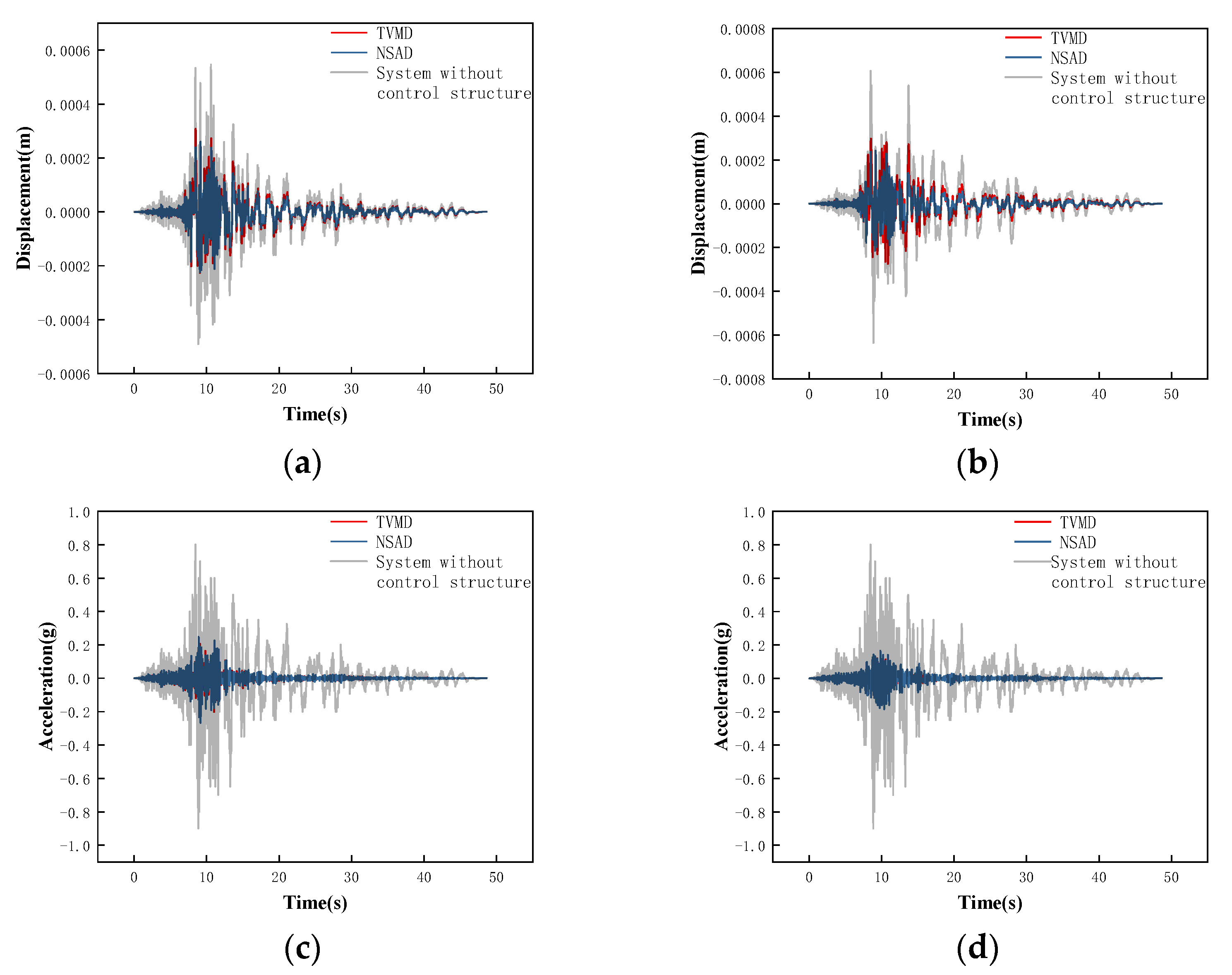
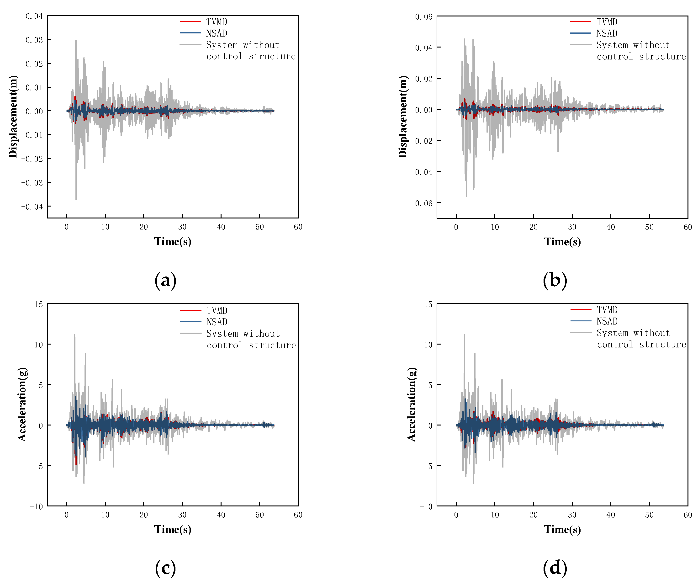
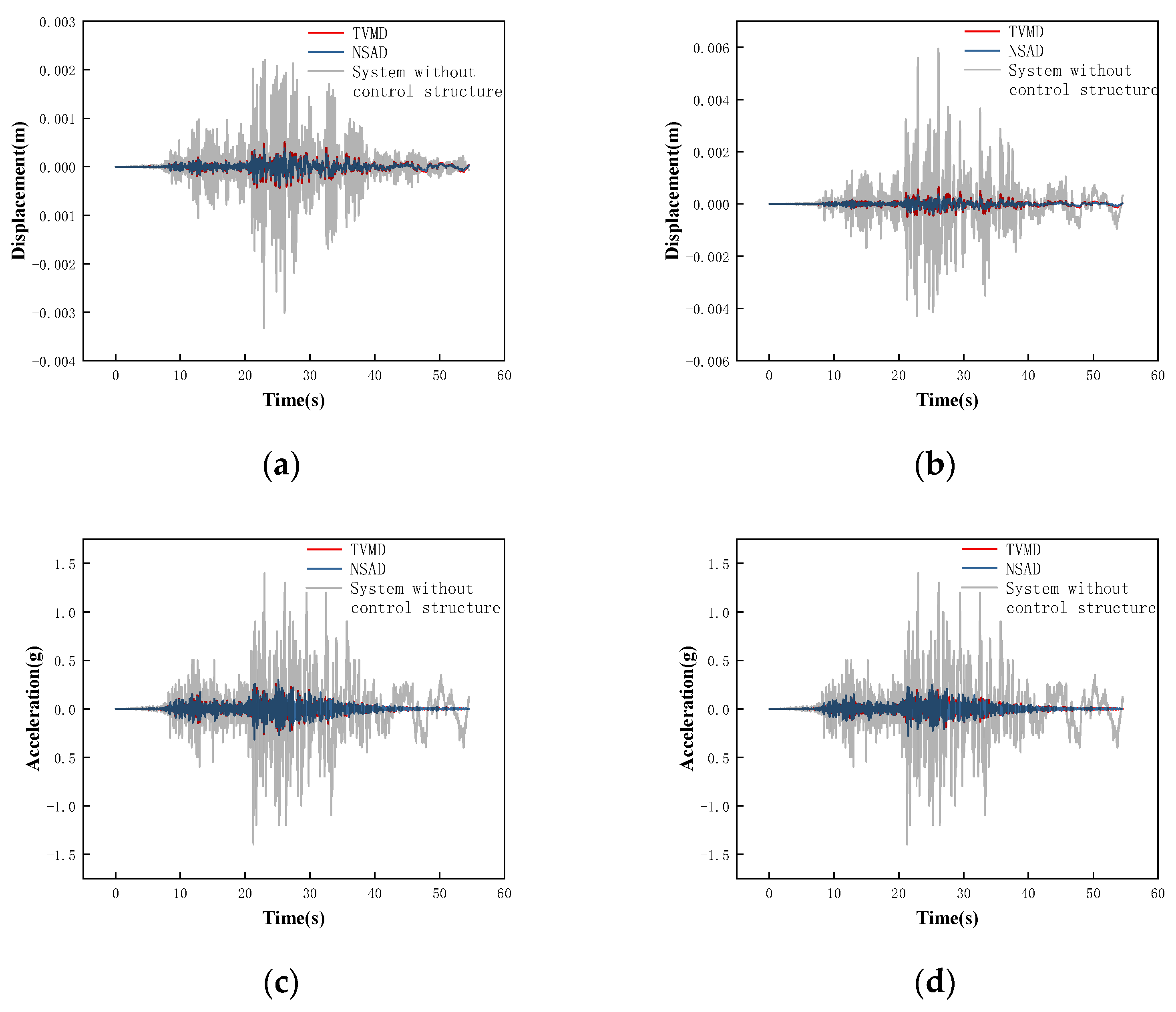
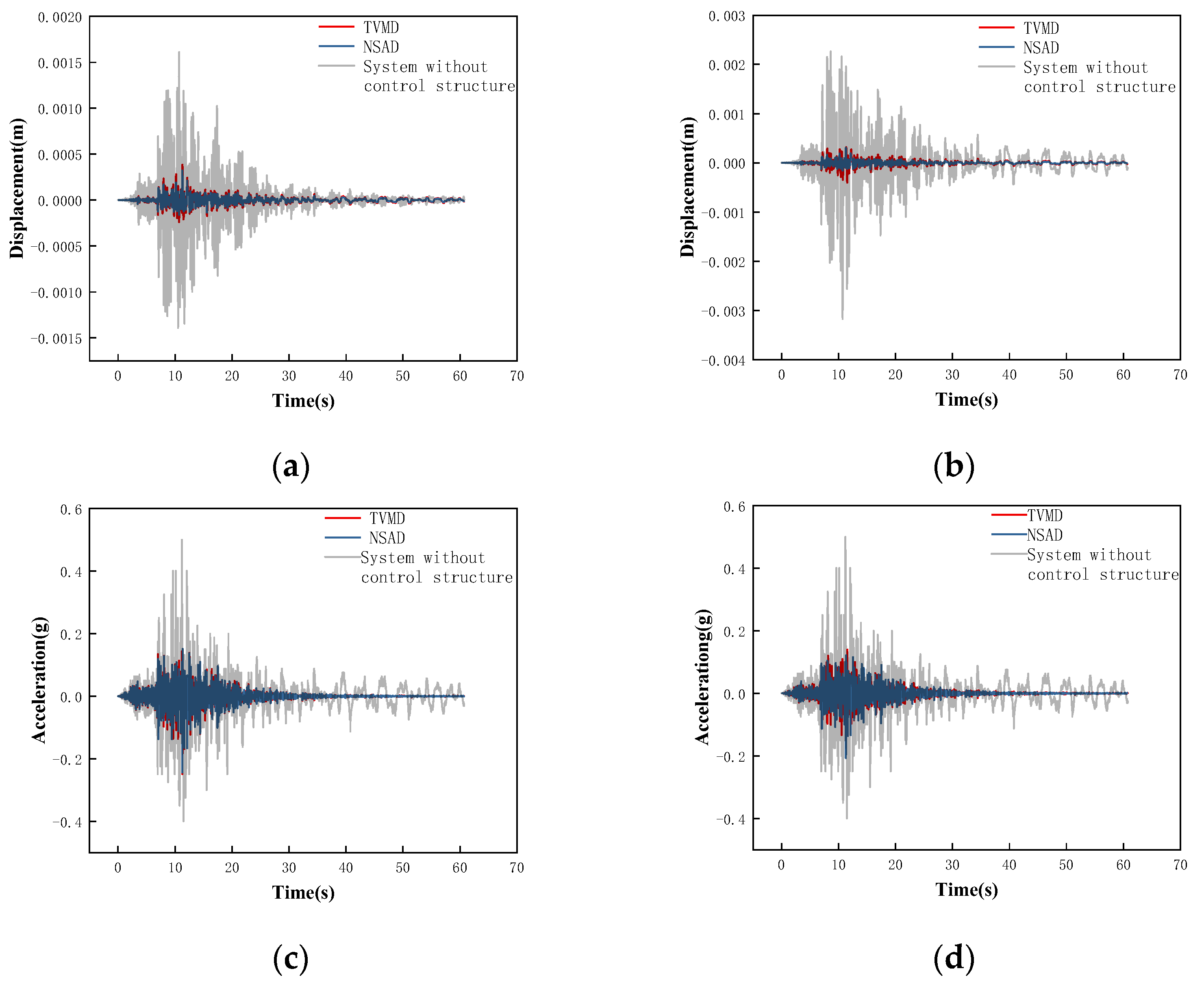
• Based on the transfer function and time-history response diagram, it is concluded that both the TVMD vibration control system and NSAD vibration control system can play a role in vibration control of adjacent building structures proposed in this paper.
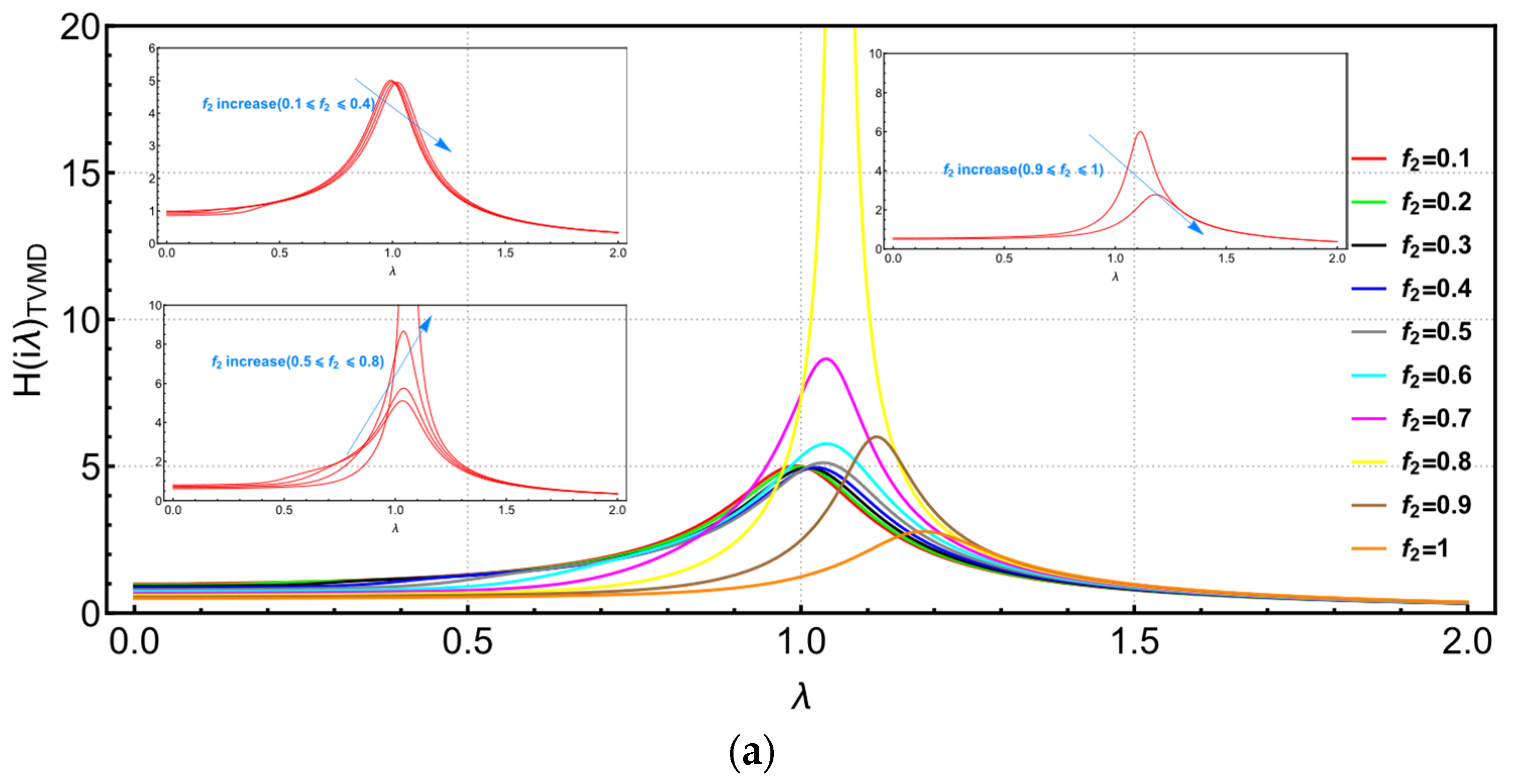
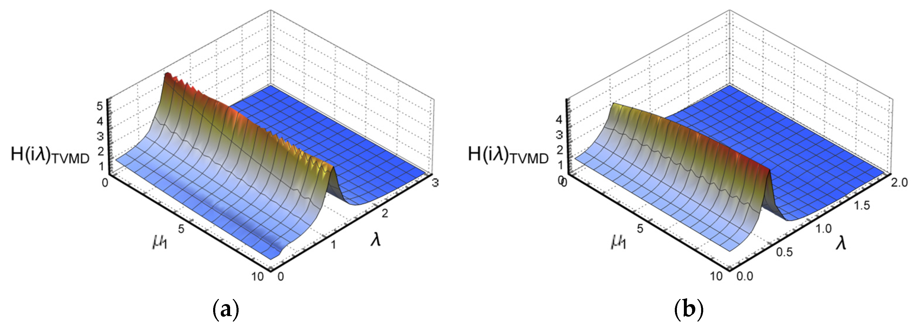
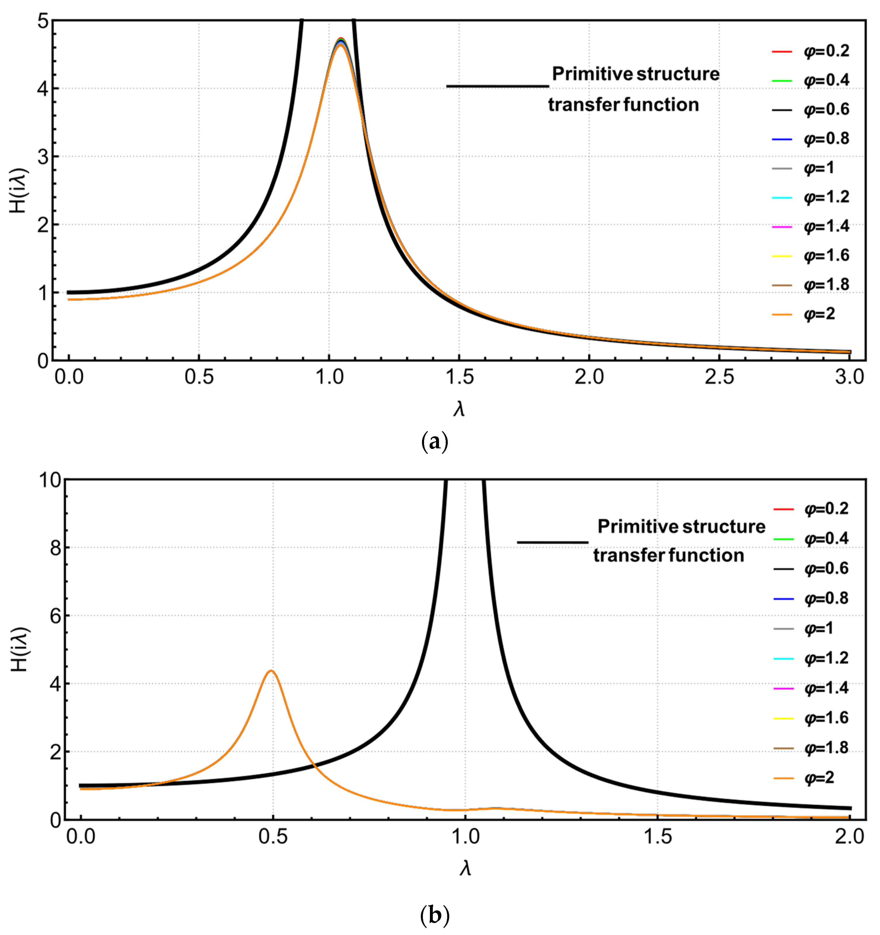
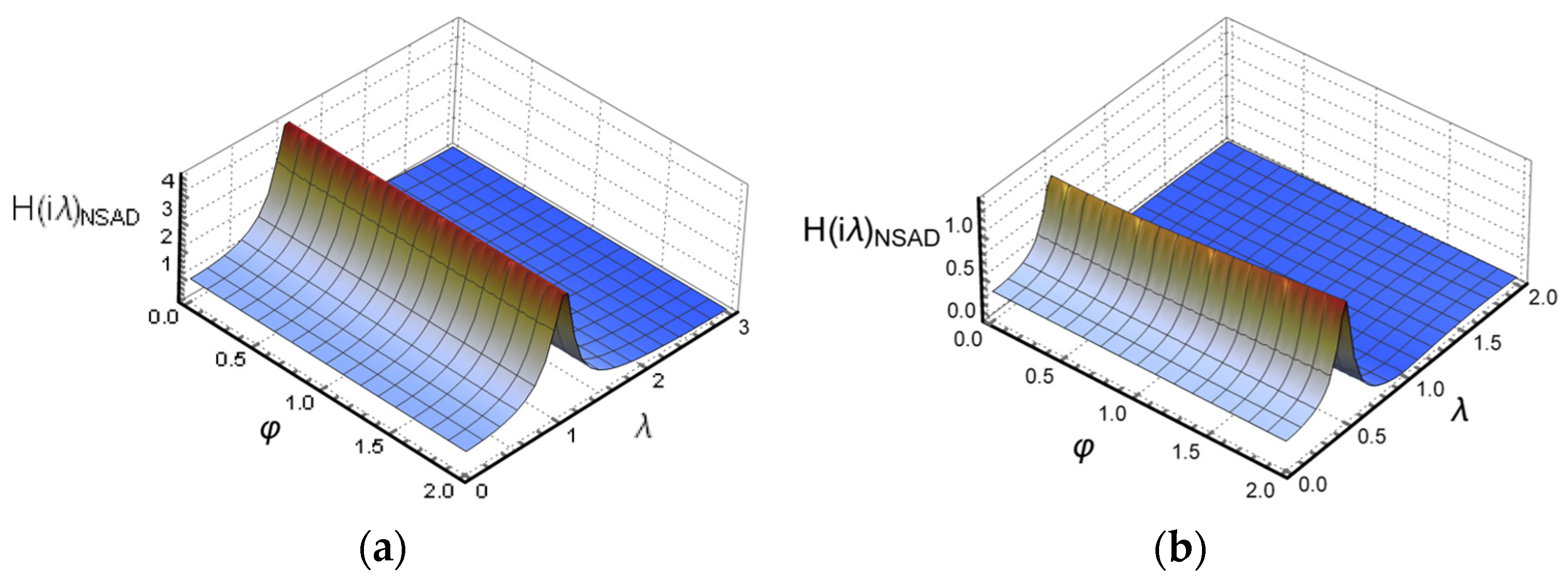
• In the TVMD vibration control system, the maximum peak value appears on the “left structure” when parameter $f_2=0.8$. When parameter $f_2=0.4$, the transfer function image has obvious troughs. As the parameter ${\mu }_1$ increases, the peak value of the transfer function on the “left structure” decreases slowly, and the peak value of the transfer function on the right of the structure increases slowly.
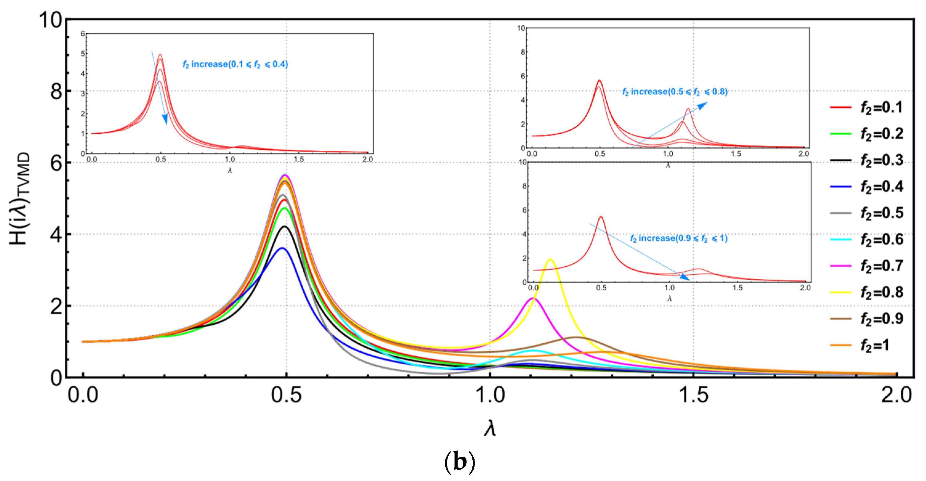
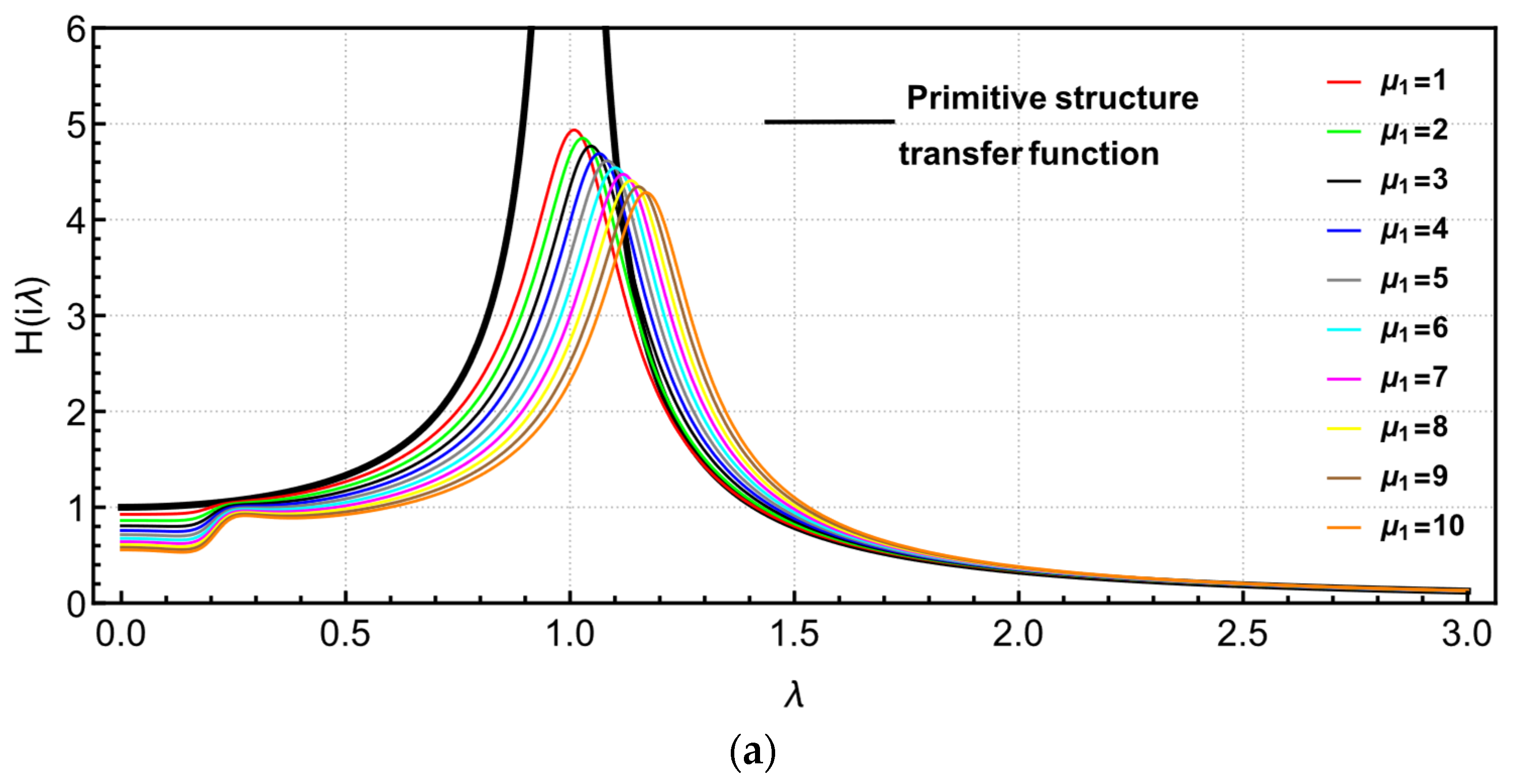
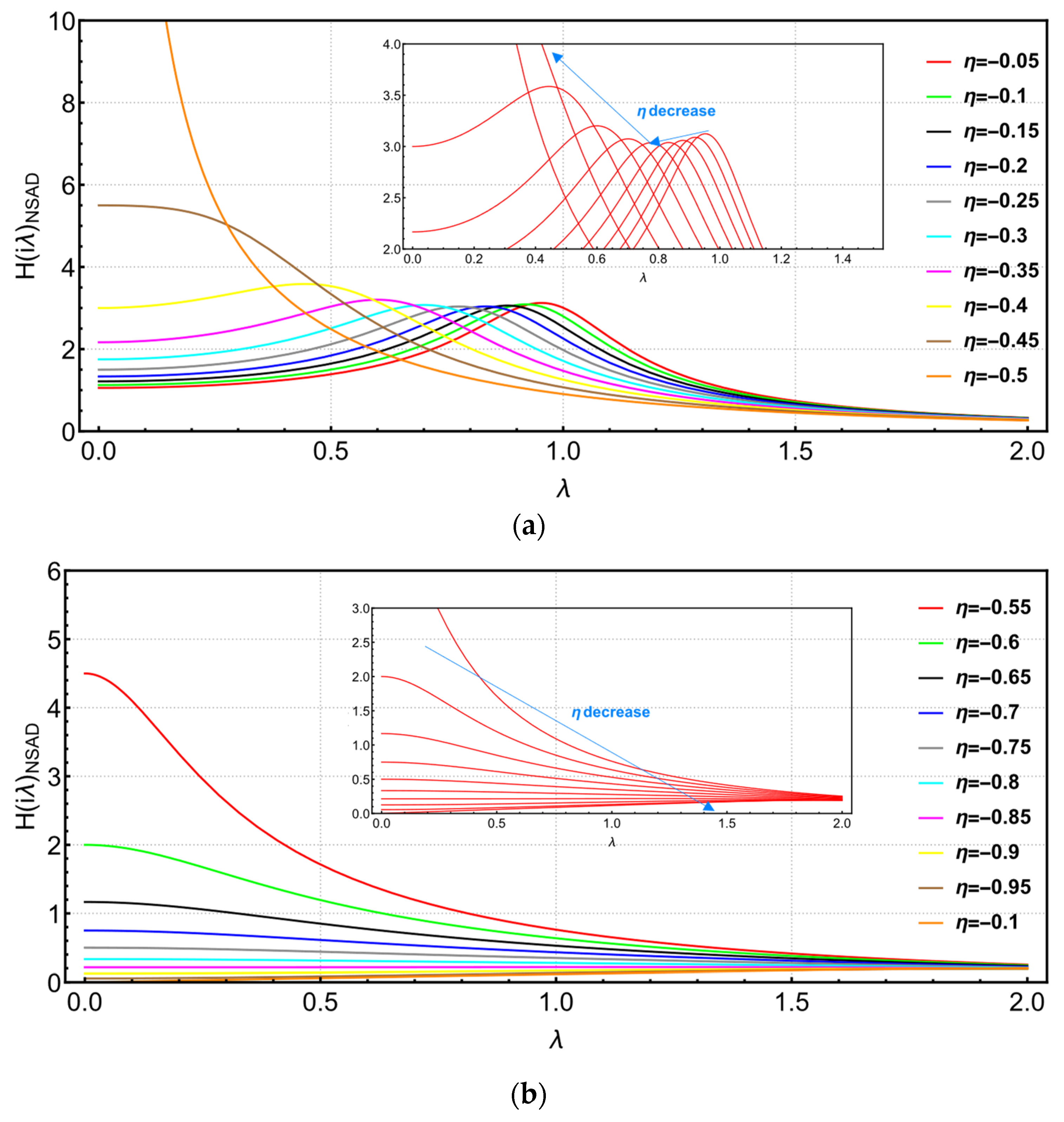
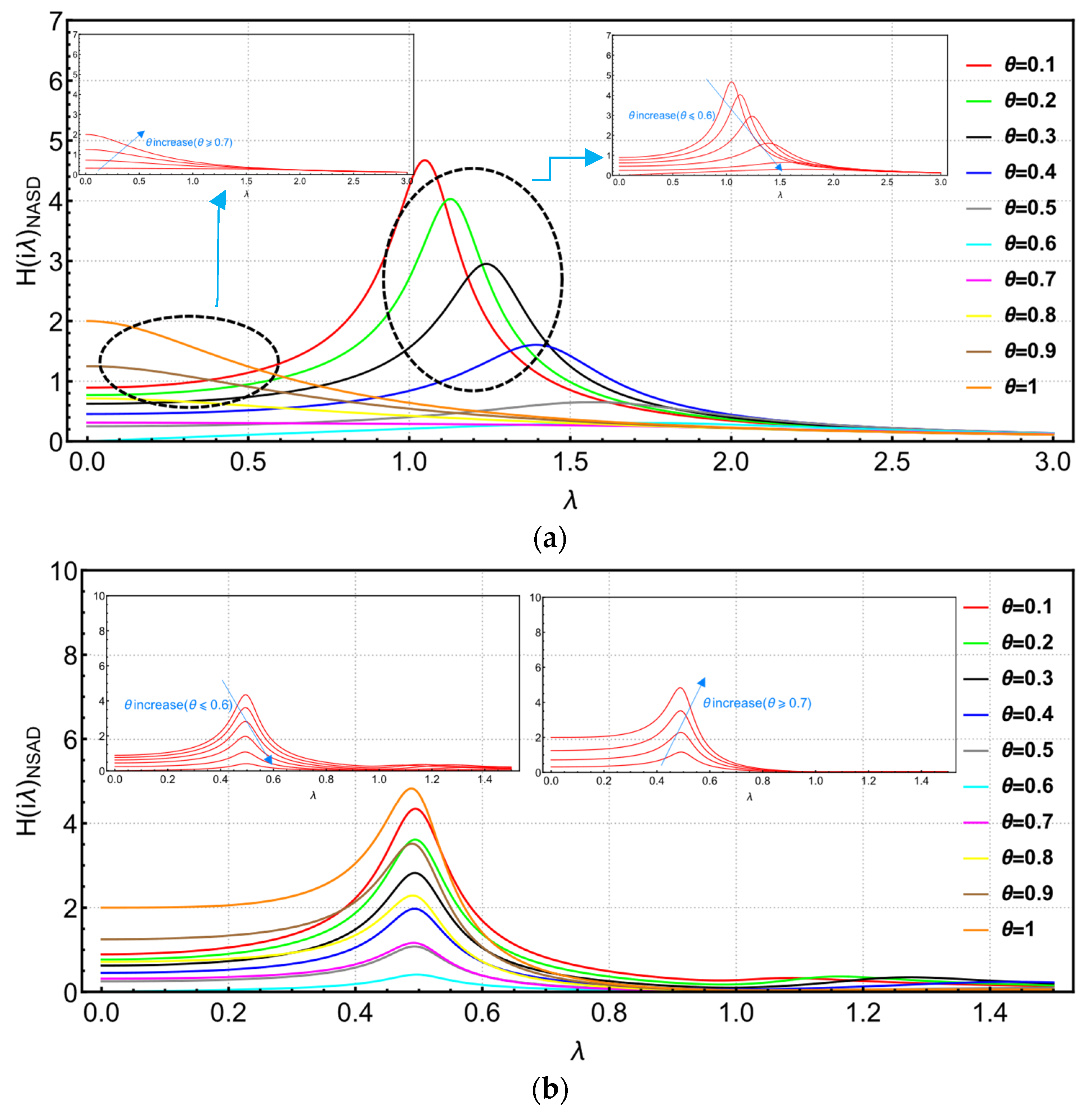
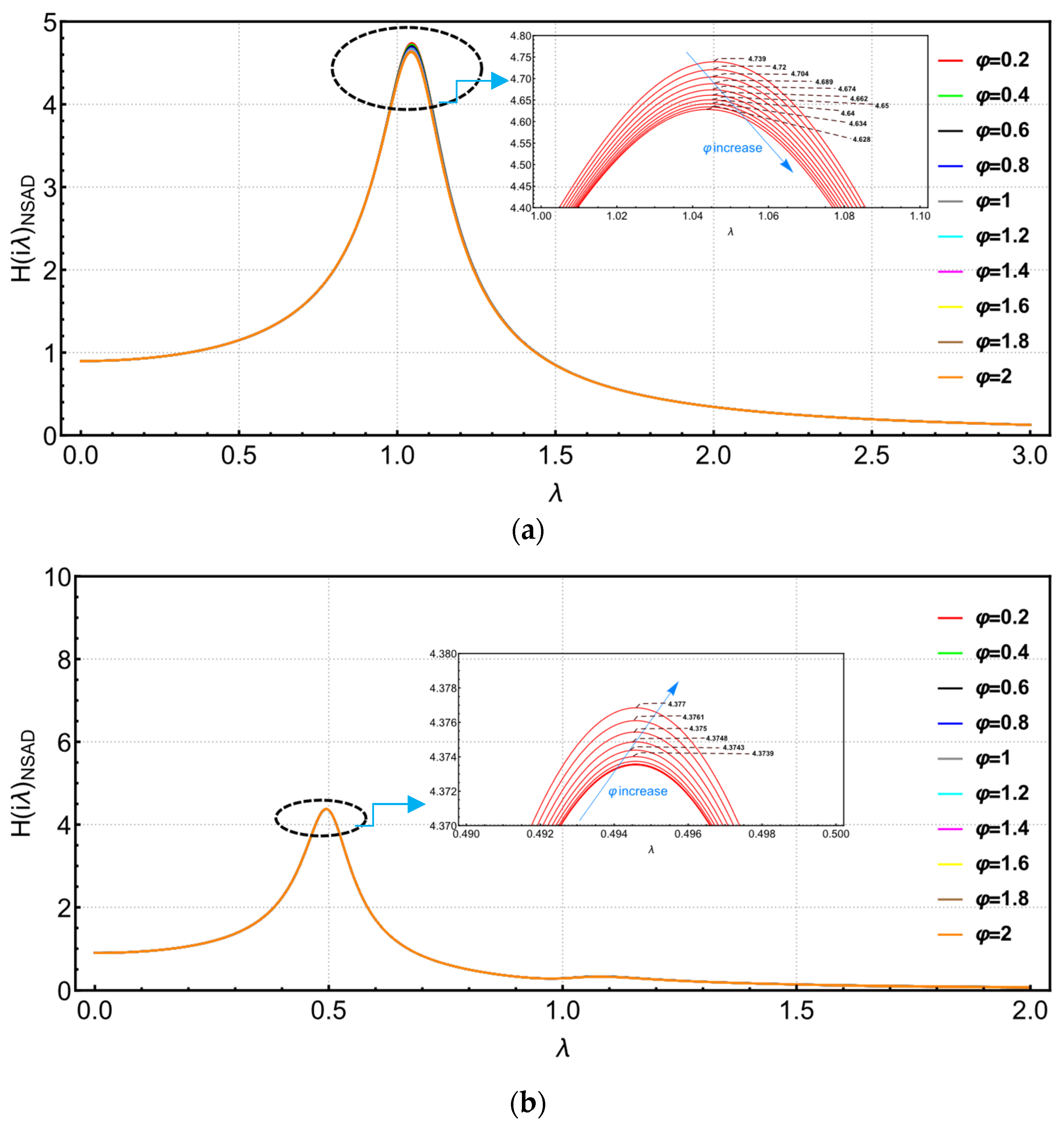
• In the NSAD vibration control system, the peaks of the “left structure” and the “right structure” transfer functions increase abruptly when $\eta =-0.5$. At $\eta =-0.5$, the peak value of the transfer function increases continuously. At $-0.5<\eta <-1$, the peak value of the transfer function decreases continuously. When parameter $\theta =0.6$, the transfer function image has obvious troughs. The parameter $\phi$ has little influence on the structure and fails to make the transfer function curve of the structure fluctuate significantly.
• In the mid-range response results in Section 5, it can be seen that the NSAD vibration control system is compared with the TVMD vibration control system. The NSAD vibration control system has good control ability in displacement response. TVMD vibration control system has better control ability than the NSAD vibration control system in terms of acceleration response. There is little difference in the acceleration response between the two systems.

In order to simplify the calculation, this paper analyzes and designs the building structure based on the linear elasticity assumption. However, the building structure has strong nonlinear properties under the action of earthquakes and other disasters, especially in the design of energy dissipation, isolation and seismic performance; ignoring the nonlinear properties of the building structure will lead to the deviation of the calculation results. Often said, nonlinearity is divided into three categories: geometric nonlinearity, material nonlinearity and state nonlinearity. Geometric nonlinearity has a great influence on the study of this paper. When the building structure deformation is large, it will cause a change in load size and direction. Therefore, the influence of displacement must be considered when establishing the structural equilibrium equation. Considering the geometric nonlinearity, the deformation changes gradually with an increase in load. The time-history response and optimization results of linear behavior are smaller than those of nonlinear behavior. The original parameter conditions will no longer apply.

References

1. Ji, X.; Kajiwara, K.; Nagae, T.; Enokida, R.; Nakashima, M. A substructure shaking table test for reproduction of earthquake responses of high-rise buildings. Soil Dyn. Earthq. Eng. 2009, 38, 1381–1399. [Google Scholar] [CrossRef]
2. Kam, W.Y.; Pampanin, S. The seismic performance of RC buildings in the 22 February 2011 Christchurch earthquake. Struct. Concr. 2011, 12, 223–233. [Google Scholar] [CrossRef]
3. Rayegani, A.; Nouri, G. Application of Smart Dampers for Prevention of Seismic Pounding in Isolated Structures Subjected to Near-fault Earthquakes. J. Earthq. Eng. 2022, 26, 4069–4084. [Google Scholar] [CrossRef]
4. Rayegani, A.; Nouri, G. Seismic collapse probability and life cycle cost assessment of isolated structures subjected to pounding with smart hybrid isolation system using a modified fuzzy based controller. Structures 2022, 44, 30–41. [Google Scholar] [CrossRef]
5. Pippi, A.; Júnior, P.B.; Avila, S.; Morais, D.; Doz, G. Dynamic Response to Different Models of Adjacent Coupled Buildings. J. Vib. Eng. Technol. 2019, 8, 247–256. [Google Scholar] [CrossRef]
6. He, T.; Jiang, N. Substructure shake table test for equipment-adjacent structure-soil interaction based on the branch mode method. Struct. Des. Tall Spec. Build. 2019, 28, 1573. [Google Scholar] [CrossRef] [Green Version]
7. Basili, M.; Angelis, M.D.; Pietrosanti, D. Defective two adjacent single degree of freedom systems linked by spring-dashpot-inerter for vibration control. Eng. Struct. 2019, 188, 480–492. [Google Scholar] [CrossRef]
8. Chau, K.T.; Wei, X.X.; Guo, X.; Shen, C.Y. Experimental and theoretical simulations of seismic poundings between two adjacent structures. Earthq. Eng. Struct. Dyn. 2003, 32, 537–554. [Google Scholar] [CrossRef]
9. Polycarpou, P.C.; Komodromos, P. Earthquake-induced poundings of a seismically isolated building with adjacent structures. Eng. Struct. 2010, 32, 1937–1951. [Google Scholar] [CrossRef]
10. Ni, Y.Q.; Ko, J.M.; Ying, Z.G. Random seismic response analysis of adjacent buildings coupled with non-linear hysteretic dampers. J. Sound Vib. 2001, 246, 403–417. [Google Scholar] [CrossRef]
11. Yang, Z.; Xu, Y.L.; Lu, X.L. Experimental seismic study of adjacent buildings with fluid dampers. J. Struct. Eng. 2003, 129, 197–205. [Google Scholar] [CrossRef]
12. Ying, Z.G.; Ni, Y.Q.; Ko, J.M. Stochastic optimal coupling-control of adjacent building structures. Comput. Struct. 2003, 81, 2775–2787. [Google Scholar] [CrossRef]
13. Bhaskararao, A.V.; Jangid, R.S. Seismic response of adjacent buildings connected with friction dampers. Bull. Earthq. Eng. 2006, 4, 43–64. [Google Scholar] [CrossRef]
14. Kim, J.; Ryu, J.; Chung, L. Seismic performance of structures connected by viscoelastic dampers. Eng. Struct. 2006, 28, 183–195. [Google Scholar] [CrossRef]
15. Zhu, H.P.; Ge, D.D.; Huang, X. Optimum connecting dampers to reduce the seismic responses of parallel structures. J. Sound Vib. 2011, 30, 1931–1949. [Google Scholar] [CrossRef]
16. Basili, M.; De Angelis, M. Optimal passive control of adjacent structures interconnected with nonlinear hysteretic devices. J. Sound Vib. 2007, 30, 106–125. [Google Scholar] [CrossRef]
17. Lu, Z.; Wang, Z.; Zhou, Y.; Lu, X. Nonlinear dissipative devices in structural vibration control: A review. J. Sound Vib. 2018, 423, 18–49. [Google Scholar] [CrossRef]
18. Christenson, R.E.; Spencer, B.F., Jr.; Johnson, E.A. Semiactive connected control method for adjacent multi-degree-of-freedom buildings. J. Eng. Mech. 2007, 133, 290–298. [Google Scholar] [CrossRef]
19. Palacios-Quiñonero, F.; Rubió-Massegú, J.; Rossell, J.M.; Karimi, H.R. Semiactive–passive structural vibration control strategy for adjacent structures under seismic excitation. J. Franklin Inst. 2012, 349, 3003–3026. [Google Scholar] [CrossRef]
20. Spencer, B.F.; Nagarajaiah, S. State of the art of structural control. J. Struct. Eng. 2003, 129, 845–856. [Google Scholar] [CrossRef]
21. Sun, F.-F.; Yang, J.-Q.; Wang, M.; Wu, T.-Y. An adaptive viscous damping wall for seismic protection: Experimental study and performance-based design. J. Build. Eng. 2021, 44, 102645. [Google Scholar] [CrossRef]
22. Platus, D.L. Negative-stiffness-mechanism vibration isolation systems. Vibration control in microelectronics. SPIE Proc. 1992, 1619, 44–54. [Google Scholar]
23. Mizuno, T.; Toumiya, T.; Takasaki, M. Vibration isolation system using negative stiffness. JSME Int. J. 2003, 46, 807–812. [Google Scholar] [CrossRef] [Green Version]
24. Iemura, H.; Pradono, M.H. Passive and semi-active seismic response control of a cable-stayed bridge. Struct. Control Health Monit. 2002, 9, 189–204. [Google Scholar] [CrossRef]
25. Iemura, H.; Pradono, M.H. Simple algorithm for semi-active seismic response control of cable-stayed bridges. Earthq. Eng. Struct. Dyn. 2005, 34, 409–423. [Google Scholar] [CrossRef]
26. Li, H.; Liu, J.; Ou, J. Seismic response control of a cable-stayed bridge using negative stiffness dampers. Struct. Control Health Monit. 2011, 18, 265–288. [Google Scholar] [CrossRef]
27. Li, H.; Liu, M.; Ou, J. Negative stiffness characteristics of active and semi-active control systems for stay cables. Struct. Control Health Monit. 2008, 15, 120–142. [Google Scholar] [CrossRef]
28. Weber, F.; Distl, H. Semi-active damping with negative stiffness for multi-mode cable vibration mitigation: Approximate collocated control solution. Smart Mater. Struct. 2015, 24, 115015. [Google Scholar] [CrossRef]
29. Gong, W.; Xiong, S. A new filter-based pseudo-negative-stiffness control for base-isolated buildings. Struct. Control Health Monit. 2017, 24, e1912. [Google Scholar] [CrossRef]
30. Hogsberg, J. The role of negative stiffness in semi-active control of magneto-rheological dampers. Struct. Control Health Monit. 2011, 18, 289–304. [Google Scholar] [CrossRef]
31. Weber, F.; Boston, C. Clipped viscous damping with negative stiffness for semi-active cable damping. Smart Mater. Struct. 2011, 20, 045007. [Google Scholar] [CrossRef]
32. Wu, B.; Shi, P.; Ou, J. Seismic performance of structures incorporating magnetorheological dampers with pseudo-negative stiffness. Struct. Control Health Monit. 2013, 20, 405–421. [Google Scholar] [CrossRef]
33. Shi, X.; Zhu, S. Magnetic negative stiffness dampers. Smart Mater. Struct. 2015, 24, 072002. [Google Scholar] [CrossRef]
34. Shi, X.; Zhu, S. Simulation and optimization of magnetic negative stiffness dampers. Sens. Actuator A Phys. 2017, 259, 14–33. [Google Scholar] [CrossRef]
35. Chen, L.; Sun, L.; Nagarajaiah, S. Cable with discrete negative stiffness device and viscous damper: Passive realization and general characteristics. Smart Struct. Syst. 2015, 15, 627–643. [Google Scholar] [CrossRef]
36. Antoniadis, I.; Chronopoulos, D.; Spitas, V.; Koulocheris, D. Hyper-damping properties of a stiff and stable linear oscillator with a negative stiffness element. J. Sound Vib. 2015, 346, 37–52. [Google Scholar] [CrossRef]
37. Kalathur, H.; Lakes, R.S. Column dampers with negative stiffness: High damping at small amplitude. Smart Mater. Struct. 2013, 22, 084013. [Google Scholar] [CrossRef]
38. Dong, L.; Lakes, R. Advanced damper with high stiffness and high hysteresis damping based on negative structural stiffness. Int. J. Solids Struct. 2013, 50, 2416–2423. [Google Scholar] [CrossRef] [Green Version]
39. Wang, M.; Sun, F.; Jin, H. Performance evaluation of existing isolated buildings with supplemental passive pseudo-negative stiffness devices. Eng. Struct. 2018, 177, 30–46. [Google Scholar] [CrossRef]
40. Lai, Z.; Sun, T.; Nagarajaiah, S. Adjustable template stiffness device and SDOF nonlinear frequency response. Nonlinear Dyn. 2019, 96, 1559–1573. [Google Scholar] [CrossRef]
41. Shen, Y.; Peng, H.; Li, X.; Yang, S. Analytically optimal parameters of dynamic vibration absorber with negative stiffness. Mech. Syst. Signal Process. 2017, 85, 193–203. [Google Scholar] [CrossRef]
42. Walsh, K.K.; Boso, E.; Steinberg, E.P.; Haftman, J.T.; Littell, W.N. Variable negative stiffness device for seismic protection of building structures through apparent weakening. J. Eng. Mech. 2018, 144, 04018090. [Google Scholar] [CrossRef]
43. Wang, M.; Sun, F.; Yang, J.; Nagarajaiah, S. Seismic protection of SDOF systems with a negative stiffness amplifying damper. Eng. Struct. 2019, 190, 128–141. [Google Scholar] [CrossRef]
44. Mathew, G.; Jangid, R.S. Seismic response control of a building by negative stiffness devices. Asian J. Civ. Eng. 2018, 19, 849–866. [Google Scholar] [CrossRef]
45. Carrella, A.; Brennan, M.J.; Waters, T.P. Demonstrator to show the effects of negative stiffness on the natural frequency of a simple oscillator. Proc. Inst. Mech. Eng. Part C J. Mech. Eng. Sci. 2008, 222, 1189–1192. [Google Scholar] [CrossRef]
46. Li, H.; Li, J.; Yu, Y.; Li, Y. Modified adaptive negative stiffness device with variable negative stiffness and geometrically nonlinear damping for seismic protection of structures. Int. J. Struct. Stab. Dyn. 2021, 21, 2150107. [Google Scholar] [CrossRef]
47. Iemura, H.; Igarashi, A.; Pradono, M.H.; Kalantari, A. Negative stiffness friction damping for seismically isolated structures. Struct. Control Health Monit. 2006, 13, 775–791. [Google Scholar] [CrossRef]
48. Toyooka, A.; Kouchiyama, O.; Iemura, H.; IKEDA, M. Development of the passive negative stiffness friction device and its verification through shaking table. Doboku Gakkai Ronbunshuu A 2010, 66, 148–162. [Google Scholar] [CrossRef] [Green Version]
49. Zhou, P.; Li, H. Modeling and control performance of a negative stiffness damper for suppressing stay cable vibrations. Struct. Control Health Monit. 2016, 23, 764–782. [Google Scholar] [CrossRef]
50. Wang, H.; Gao, H.; Li, J.; Wang, Z.; Ni, Y.; Liang, R. Optimum design and performance evaluation of the tuned inerter-negative-stiffness damper for seismic protection of single-degree-of-freedom structures. Int. J. Mech. Sci. 2021, 212, 106805. [Google Scholar] [CrossRef]
51. Wang, M.; Sun, F.-F.; Nagarajaiah, S. simplified optimal design of MDOF structures with negative stiffness amplifying dampers based on effective damping. Struct. Des. 2019, 28, e1664. [Google Scholar] [CrossRef]
52. Pasala, D.T.R.; Sarlis, A.A.; Reinhorn, A.M.; Nagarajaiah, S.; Constantinou, M.C.; Taylor, D. Simulated bilinear-elastic behavior in a SDOF elastic structure using negative stiffness device: Experimental and analytical study. J. Struct. Eng. 2014, 140, 04013049. [Google Scholar] [CrossRef]
53. Pasala, D.T.R.; Sarlis, A.A.; Reinhorn, A.M.; Nagarajaiah, S.; Constantinou, M.C.; Taylor, D. Apparent weakening in SDOF yielding structures using a negative stiffness device: Experimental and analytical study. J. Struct. Eng. 2015, 141, 04014130. [Google Scholar] [CrossRef]
54. Zhao, Z.; Chen, Q.; Hu, X.; Zhang, R. Enhanced energy dissipation benefit of negative stiffness amplifying dampers. Int. J. Mech. Sci. 2023, 240, 107934. [Google Scholar] [CrossRef]
55. Kang, X.; Li, S.; Hu, J. Design and parameter optimization of the reduction-isolation control system for building structures based on negative stiffness. Buildings 2023, 13, 489. [Google Scholar] [CrossRef]
Figure 1. Adjacent structure building model.
Buildings 13 02049 g001
Figure 2. Simplified model of adjacent building structure.
Buildings 13 02049 g002
Figure 3. The influence of frequency ratio f 2 on H T V M D l / r λ . (a) H T V M D l λ ; (b) H T V M D r λ .
Buildings 13 02049 g003aBuildings 13 02049 g003b
Figure 4. The comparison between the transfer function of parameter f 2 in TVMD vibration control system and the original structure transfer function. (a) H T V M D l   λ compared to H l λ ; (b) H T V M D r   λ compared to H r λ .
Buildings 13 02049 g004
Figure 5. The influence of mass ratio μ 1 on H T V M D l / r λ . (a) H T V M D l λ ; (b) H T V M D r λ .
Buildings 13 02049 g005
Figure 6. The comparison between the transfer function of parameter μ 1 in the TVMD vibration control system and the original structure transfer function. (a) H T V M D l   λ compared to H l λ ; (b) H T V M D r   λ compared to H r λ .
Buildings 13 02049 g006aBuildings 13 02049 g006b
Figure 7. Three-dimensional curve of parameter f 2 in the TVMD vibration control system. (a) left structure; (b) right structure.
Buildings 13 02049 g007
Figure 8. Three-dimensional curve of parameter μ 1 in the TVMD vibration control system. (a) left structure; (b) right structure.
Buildings 13 02049 g008
Figure 9. The influence of negative stiffness ratio η on H N S A D l / r λ . (a) H N S A D l λ   ( η > 0.5 ) ; (b) H N S A D l λ   ( η < 0.5 ) ; (c) H N S A D r λ   ( η > 0.5 ) ; (d) H N S A D r λ   ( η < 0.5 ) .
Buildings 13 02049 g009aBuildings 13 02049 g009b
Figure 10. The comparison between the transfer function of parameter η and the original structure of the NSAD vibration control system. (a) H N S A D l   λ compared to H l λ   ( η > 0.5 ) ; (b) H N S A D l   λ compared to H l λ   ( η < 0.5 ) ; (c) H N S A D r   λ compared to H r λ   ( η > 0.5 ) ; (d) H N S A D r   λ compared to H r λ   ( η < 0.5 ) .
Buildings 13 02049 g010aBuildings 13 02049 g010b
Figure 11. The influence of additional stiffness ratio θ on H N S A D l / r λ . (a) H N S A D l λ ; (b) H N S A D r λ .
Buildings 13 02049 g011
Figure 12. The comparison between the transfer function of parameter θ and the original structure of the NSAD vibration control system. (a) H N S A D l   λ compared to H l λ ; (b) H N S A D r   λ compared to H r λ .
Buildings 13 02049 g012aBuildings 13 02049 g012b
Figure 13. The influence of additional damping ratio φ on H N S A D l / r λ . (a) H N S A D l λ ; (b) H N S A D r λ .
Buildings 13 02049 g013
Figure 14. The comparison between the transfer function of parameter φ and the original structure of the NSAD vibration control system. (a) H N S A D l   λ compared to H l λ ; (b) H N S A D r   λ compared to H r λ .
Buildings 13 02049 g014
Figure 15. Three-dimensional curve of the parameter η in the NSAD vibration control system. (a) left structure; (b) right structure.
Buildings 13 02049 g015
Figure 16. Three-dimensional curve of the parameter θ in the NSAD vibration control system. (a) left structure; (b) right structure.
Buildings 13 02049 g016
Figure 17. Three-dimensional curve of the parameter φ in the NSAD vibration control system. (a) left structure; (b) right structure.
Buildings 13 02049 g017
Figure 18. Monte Carlo method calculation flow chart.
Buildings 13 02049 g018
Figure 19. Contour diagram of TVMD vibration control system parameters.
Buildings 13 02049 g019
Figure 20. Contour diagram of NSAD vibration control system parameters.
Buildings 13 02049 g020
Figure 21. Seismic analysis results of the Chi-Chi Earthquake wave. (a) displacement response of the “left structure”; (b) displacement response of the “right structure”; (c) acceleration response of the “left structure”; (d) acceleration response of the “right structure”.
Buildings 13 02049 g021
Figure 22. Seismic analysis results of the Chuetsu-Oki Earthquake wave. (a) displacement response of the “left structure”; (b) displacement response of the “right structure”; (c) acceleration response of the “left structure”; (d) acceleration response of the “right structure”.
Buildings 13 02049 g022
Figure 23. Seismic analysis results of the Darfield New Zealand Earthquake wave. (a) displacement response of the “left structure”; (b) displacement response of the “right structure”; (c) acceleration response of the “left structure”; (d) acceleration response of the “right structure”.
Buildings 13 02049 g023
Figure 24. Seismic analysis results of the EL Centro Earthquake wave. (a) displacement response of the “left structure”; (b) displacement response of the “right structure”; (c) acceleration response of the “left structure”; (d) acceleration response of the “right structure”.
Buildings 13 02049 g024
Figure 25. Seismic analysis results of the EL Mayor-Cucapsh Earthquake wave. (a) displacement response of the “left structure”; (b) displacement response of the “right structure”; (c) acceleration response of the “left structure”; (d) acceleration response of the “right structure”.
Buildings 13 02049 g025
Figure 26. Seismic analysis results of the Imperial Valley Earthquake wave. (a) displacement response of the “left structure”; (b) displacement response of the “right structure”; (c) acceleration response of the “left structure”; (d) acceleration response of the “right structure”.
Buildings 13 02049 g026
Figure 27. Seismic analysis results of the Irpinia Italy Earthquake wave. (a) displacement response of the “left structure”; (b) displacement response of the “right structure”; (c) acceleration response of the “left structure”; (d) acceleration response of the “right structure”.
Buildings 13 02049 g027
Figure 28. Seismic analysis results of the Iwate Earthquake wave. (a) displacement response of the “left structure”; (b) displacement response of the “right structure”; (c) acceleration response of the “left structure”; (d) acceleration response of the “right structure”.
Buildings 13 02049 g028
Figure 29. Seismic analysis results of the Kobe Japan Earthquake wave. (a) displacement response of the “left structure”; (b) displacement response of the “right structure”; (c) acceleration response of the “left structure”; (d) acceleration response of the “right structure”.
Buildings 13 02049 g029
Figure 30. Seismic analysis results of the San Fernando Earthquake wave. (a) displacement response of the “left structure”; (b) displacement response of the “right structure”; (c) acceleration response of the “left structure”; (d) acceleration response of the “right structure”.
Buildings 13 02049 g030