Abstract
The specific air jet of a diffuser is formed by the complex internal structure, which affects the outlet airflow distribution of the diffuser directly and the indoor environment distribution indirectly. If the diffusers are developed based on their actual geometry structure and their boundary conditions are set as their inlet flowrate, the simulated indoor temperature distribution will be more accurate. However, it is noted that many problems may arise, such as model complexity, many grid cells, and slow convergence of calculations. Therefore, this paper focuses on a simplified method for four-way square diffusers in a computational fluid dynamics (CFD) simulation of indoor non-uniform temperature distribution. Firstly, the airflow distribution is simulated on the outlet air supply cross-section of the diffuser. Then, according to the outflow characteristics of the diffuser, the diffuser model is simplified and simulated in an experimental room. Finally, the temperature distribution at the 1.2 m height plane is obtained from CFD simulation and compared with the experimental results. The results show that the 68-point air supply opening model can well simulate the effects of the outlet airflow distribution of the diffuser, and the simulated indoor temperature distribution meets the experiment results well. The deviations for three scenarios are between −7.4~1.7% and the average deviation is −3.0%, while the root mean square error of temperature for three scenarios is 0.7 °C, 0.7 °C, and 1.0 °C, respectively. The results also demonstrate the mutual influence of the airflow from different diffusers and the indoor non-uniform temperature distribution under the action of multiple diffusers. The proposed method can contribute to balancing the model complexity and the accuracy in CFD simulation, especially for multiple diffusers in the room.
1. Introduction
In terms of design and control strategy optimization of heating, ventilation, and air conditioning (HVAC) systems, indoor temperature is usually considered uniformly distributed. Actually, the indoor temperature is non-uniform and affected by dynamic outdoor environments [1], non-uniform internal load distribution [2], and varying indoor airflow patterns [3]. Meanwhile, with the increasing requirements of personal thermal comfort, the thermal comfort of the human-centered micro-environment is more important than that for the whole room [4,5]. Human thermal comfort is mainly affected by the airflow rate [6], the non-uniform distribution of indoor temperature [7,8], and the thermal radiation from the environmental surface [9], while the former two factors have a direct relationship with the condition of supply airflow [10,11].
Diffusers are the terminals of the air conditioning system, while the specific air jet results from the complex internal structure of the diffusers, which will dominate the room air movement. Therefore, the jet effect of the diffuser is an important factor affecting the indoor environment [12,13]. With the development of computers, computational fluid dynamics (CFD) simulation has been widely used for evaluating indoor environments [14,15]. Many scholars have numerically studied and analyzed the air distribution of diffusers. Aziz et al. [16] studied the airflow characteristics of diffusers with different geometry structures (i.e., vortex, round, and square). Their effects on the indoor thermal comfort were analyzed through both numerical and experimental methods. Nocente et al. [17] conducted a numerical simulation to characterize the impact of diffuse ceiling ventilation on the internal comfort of a typical office room and compared the performance between continuous and non-continuous diffuser designs. Li et al. [18] studied the uniform and non-uniform velocity inlet boundary conditions for simulating diffusers, as well as the effects of different boundary conditions on the jet characteristics and airflow distribution.
The boundary conditions of air supply openings have a significant impact on indoor airflow during CFD simulation [19,20]. Most diffusers are much smaller than the size of the room. If the diffusers are developed based on their actual geometry structure and their boundary conditions are set as their inlet flowrate, the simulated indoor temperature distribution will be more accurate. However, it is noted that many problems can arise, such as model complexity [21], many grid cells [22], and slow convergence of calculations [23,24]. To improve simulation accuracy, proper specification of diffuser boundary conditions is crucial. Several studies have focused on developing diffuser models to enhance the representation of boundary conditions for CFD simulations.
The simulation method of supply openings was described firstly by Peter Nielsen in 1992 [25]. Then, simplified methods for diffuser simulation were proposed by Srebric and Chen in 2002 [26]. The simplest method considers the diffuser as a plane inlet, which is only based on the criterion of energy conservation with the simulation target of the average value of the indoor temperature, but neglects the non-uniform temperature distribution. Li et al. improved this simplest model in 2006 [27] and proposed the real diffuser as an N-point air supply opening model to reduce the number of grids. The number of N determines the consideration degree of the supply airflow distribution (i.e., the airflow directions) and N is suggested to be from 4 to 8. The higher the consideration degree of the airflow distribution, the more detailed the jet characteristics of the diffuser in different directions can be described, which will help to simulate the indoor non-uniform temperature field as closely as possible. Therefore, the trade-off between the setting of the N value and the computing efficiency should be further discussed.
From the above review, it is clear that the previous CFD studies of various simplified models still have several shortcomings: (1) Most of these studies considered the diffuser velocity as an even velocity based on the fully open area [28,29], simplifying or even ignoring the advection effect of diffusers. In practice the outflow from the diffuser is non-uniform and complex due to turbulent air flow and depends on the geometry characteristics of the diffuser. (2) Few diffuser modelling methods are suitable for detailed predictions of indoor non-uniform temperature distributions. The supply airflow of each terminal is not independent within the room, but rather has a mutual influence due to the air movement. The airflow distribution on the outlet cross-section of the diffuser directly determines the mixing effect of neighboring airflows, which has an impact on the indoor temperature distribution [30,31]. The current methods do not fully consider the mutual influence among diffusers and their co-impacts on indoor temperature distribution.
To address the issues, this paper focuses on a simplified simulation method for common four-way square diffusers in CFD simulations of indoor non-uniform temperature distribution. The method is based on analyzing the airflow distribution on the outlet air supply cross-section of the diffuser. This simplified method for diffusers was also applied in a room simulation and validated with the experimental results. Finally, we confirmed that a simplified method for diffusers can reduce the computing time while maintaining simulation accuracy.
2. Methods
Figure 1 shows the framework of the proposed simplified simulation method for diffusers and indoor non-uniform temperature distribution. Firstly, the airflow distribution on the outlet air supply cross-section of the four-way square diffuser is simulated, and we divide the outlet air supply cross-section into small faces according to their characteristics. Then, the model of the diffuser is simplified to the 68-point air supply opening model and simulated in an experimental room. Finally, the temperature distribution at the 1.2 m height plane is obtained from CFD simulation and is validated with the experimental results.
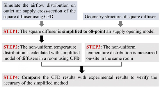
Figure 1.
Framework of this paper.
2.1. Numerical Simulation and Analysis
2.1.1. Simulation of Airflow Distribution on the Outlet Cross-Section of a Diffuser
As the outlet airflow of a four-way square diffuser is peripherally radiated to the surrounding area, accurately obtaining the airflow distribution on the diffuser air supply cross-section is important. We firstly simulated the free outlet airflow distribution of the diffuser (FOUNDATION, Suzhou, China). The size of the diffuser was 200 mm × 200 mm, and the diffuser was developed completely according to its actual geometry and internal structure, as shown in Figure 2.
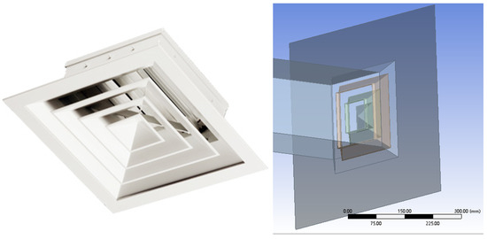
Figure 2.
Geometry model of the diffuser.
We assumed that the inlet of the diffuser (267 mm × 267 mm × 530 mm) was a straight pipe and the length of inlet pipe was twice the length of the pipe diameter to form a stable inlet flow. Meanwhile, to avoid the influence of the external area on the diffuser outlet airflow distribution, the outlet of the diffuser was set to be an infinite fluid area, so the outlet of the diffuser was set to be a cylindrical fluid area R3 000 mm × 3500 mm, as shown in Figure 3. According to the internal structure of the four-way square diffuser, its guide vanes separated the outlet section of the diffuser into three circles: outer, middle, and inner.
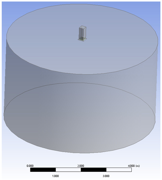
Figure 3.
Geometry model of the diffuser and the room.
For the numerical calculations, a three-dimensional (3D) model was established using Workbench2021 R2, whose mesh was generated via polyhedral cells. The diffuser was subjected to a local encryption of the mesh by 2 mm, whose maximum grid size was 50 mm, and there were altogether 3 boundary layers. To eliminate the influence of grid density on the calculation results, a grid independence test of the model was carried out, which adopted three sets of grids: coarse, medium, and fine. The calculation results under different grids were basically consistent. The difference in calculation results between medium grid and fine grid was relatively small, so considering the calculation accuracy and computational effort, a medium scale grid division was applied to the model and the total mesh number was 1,565,254.
The simulation was carried out using ANSYS FLUENT 2020 R2 [32] with the CFD modeling method and the ANSYS FLUENT solver with double precision. Fluid flow was modeled based on 3D, steady state continuity, and momentum equations. SST k-omega (2 eqn) model [33,34] was used to describe the turbulence. Since the focus was on the outlet airflow distribution of the diffuser, the energy equation was not utilized. The standard wall function was used to model the flow near the wall. For boundary conditions, the inlet section of the diffuser was set up as a velocity inlet and the outlet was a free-pressure outlet. The simulations were performed for the solver setup shown in Table 1 [35,36]. The convergence criterions of the steady state solution were defined so that the residual error for continuity, for x-, y-, and z-velocity, for k, and for omega should be under 10−3.

Table 1.
Solver setup and fluid properties used in the analysis.
When the airflow was defined in the straight inlet section of the diffuser, we could conduct calculations to obtain the airflow distribution in the outlet section of the diffuser. Figure 4 shows the results of the airflow distribution in the outlet section of the diffuser with an air volume of 295 m3·h−1. From Figure 4a, it can be seen that the airflow in the outlet section of the diffuser had an angle greater than 45 degrees to the Z-axis, and spread in all directions in a radial shape; Figure 4b shows that the velocity distribution of each circle was different due to the guide effect of the blades on each circle, and there was a return area in the center of the diffuser; Figure 4c shows the velocity vector of the outlet cross-section of the diffuser, and the velocities in its four corners decreased sharply.
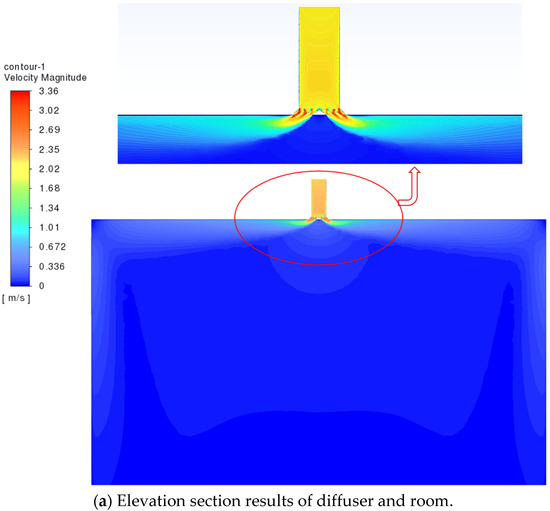
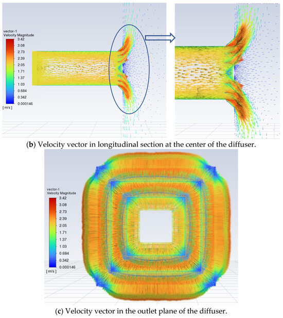
Figure 4.
The airflow distribution on the outlet section of the diffuser with 295 m3·h−1 air volume.
Concerning the airflow distribution characteristics of the diffuser’s outlet section, we divided the four corners of each circle into four squares and divided the remaining part of each edge of each circle into an even number of subfaces close to the size of a square. Then, the final diffuser’s air supply section was divided into 68 subfaces. Table 2 shows the results of the outlet cross-section of a single diffuser with an airflow of 295 m3·h−1.
Table 2.
Airflow distribution data for the outlet cross-section of the 68-point momentum model of the diffuser (air supply 295 m3·h−1).
Furthermore, according to its airflow symmetry, we took half of the sides of the outer, middle, and inner circles to quantitatively analyze the characteristics of the airflow distribution in the outlet section of the diffuser, as shown in Figure 5. The length of the arrow on each subsurface of Figure 5a indicates the numerical size of the exit airflow component, while the direction of the arrow indicates the projection angle of the exit airflow. The left side of Figure 5a shows the projection of the air supply airflow on the exit cross-section, with 45-degree directional jets and the smallest jet velocities on all four corners. Overall, the angle of the air supply airflow at the three circles was uniformly radial in the XY plane, but the velocity of the air supply airflow was non-uniform in the XY plane. The right side of Figure 5a shows the projection of the supply airflow perpendicular to the outlet section, thus the angle was uniform. However, the airflow velocity was non-uniform, and the jet velocity was the minimum on the four corners. Figure 5b shows a rose diagram of the airflow distribution for 68 subfaces, with 15-degree intervals. The 68 subfaces are cumulative based on their airflow vectors by decomposing the airflow to two nearby angles. The four corners of the diffuser are 45 degrees, 135 degrees, 225 degrees, and 315 degrees of the rose diagram, which shows that the airflow distribution on the outlet cross-section was also very uneven.


Figure 5.
Numerical analysis of 68 subfaces of the diffuser outlet cross-section.
With the influence of the complex structure inside the diffuser, the air supply flow was radiated to the surroundings in the form of advection, and had a certain regularity.
Similarly, the simulation calculations were carried out with the diffuser delivering an air volume of 213 m3·h−1, and the results of the distribution of the airflow in the outlet cross-section could be obtained. The characteristics of the diffuser were consistent with those of one delivering an air volume of 295 m3·h−1.
In view of the complex non-uniform airflow distribution in the outlet cross-section of the diffuser, when we simulated the four-way square diffusers in the room (Figure 6a), we divided the diffuser outlet air supply cross-section into 68 subsurfaces based on the geometry, as shown in Figure 6b. The diffuser model was simplified to 68 surfaces using the N-point air supply opening model, and N = 68, as shown in Figure 6c. The airflow velocities in each of the three directions XYZ for the 68 subfaces can be defined during the simulation calculation.
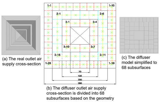
Figure 6.
Schematic diagram for the 68-point air opening model of the four-way square diffuser.
2.1.2. Simulation of the Temperature Distribution Field with Simplified Diffusers
ANSYS FLUENT 2020 R2 was used to simulate the temperature distribution field at a 1.2 m working surface height, simplifying the diffusers as a 68-point air supply opening model.
The geometry features of the experimental room, including the distribution of indoor heat sources, and the size and location of the return air outlet, were constructed in Workbench2021 R2, and both diffusers were modeled as a 68-point air supply opening model, as in Figure 7. The computational region was discretized using a polyhedral mesh with a locally encrypted 1-mm mesh for the diffuser air supply cross-section, a locally encrypted 1 mm mesh for the heat source surface, and a locally encrypted 5 mm mesh for the return air outlet. The maximum size of the grid was 0.2 m, and there were 3 boundary layers in total. The simulation began with mesh sensitivity analysis, starting with a very general computational network, improving it gradually to find the best balance between accuracy and computational effort. The final model grid is shown in Figure 8, with a grid orthogonal mass of 0.2.
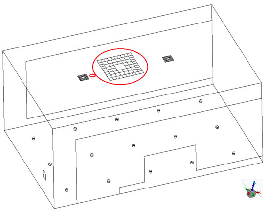
Figure 7.
68-point air supply opening model of four-way square diffusers.
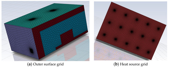
Figure 8.
Model mesh.
The ANSYS FLUENT 2020 R2 solver was set up with double precision. Fluid flow was modeled based on 3D, steady state continuity, and momentum equations. The simulations were performed for the solver setup shown in Table 1. The internal load was set according to the power of the electric stoves, which was 200 W/each. The return air was set as a pressure-free outlet that maintains a certain positive pressure in the room. The internal load density, positive pressure, and the size of the return air outlet were set according to three different experimental conditions. The 68 subfaces of the diffuser air supply cross-section were set according to Table 2 and Table 3. For boundary conditions, the ceiling and the floor were defined as adiabatic surfaces, and the glass and plasterboard walls were defined according to the properties of materials and ambient temperature, as shown in Table 4.
Table 3.
Airflow distribution data for the outlet cross-section of the 68-point momentum model of the diffuser (air supply 213 m3·h−1).
Table 4.
Building envelope and internal loads.
The convergence criterions of the steady state solution were defined so that the residual error for continuity, for x-, y-, and z-velocity, for k, and for epsilon should be under 10−3 and the residual error for energy should be under 10−6. In addition, two convergence conditions were added to the model. Under the circumstance that the variation gradient of the average temperature in the 1.2 m height plane within 10 steps and 100 steps were both less than 0.1 °C, and the number of calculation steps must be more than 2000 steps, the calculation was considered to converge, and the indoor non-uniform temperature distribution was stable.
2.2. Experimental Measurement
To validate the simplified method, a series of experiments were carried out on 12 May, 2023, in Jiading District, Shanghai, China. A 4.2 m × 6.4 m × 2.8 m room in the inner area was selected for experiments, with two side elevations dominated by transparent white glass, and the other two side elevations composed of double-layer gypsum board. Two 200 mm × 200 mm four-way square diffusers were installed on the ceiling of the room, while a strip return air outlet was installed on one plasterboard side elevation. In addition, several small electric stoves were evenly arranged on the floor as the indoor heat sources. The whole experiment was carried out at night in the spring to ensure that the air supply temperature and the ambient temperature outside the experimental room were basically unchanged during the experimental period. Meanwhile, the experimental room was not affected by solar radiation.
Theoretically, the indoor air velocity flow field between the simulation and experiment results should be compared, but this paper just compares the indoor temperature field between them to validate the proposed simplified method based on the following reasons: (1) indoor 3D wind speed is not easy to measure, (2) if anemometers are placed, the indoor flow field will be damaged, causing inaccurate measurement results, and (3) the temperature automatic recorders will have a smaller impact on the indoor temperature field. Altogether, 20 temperature automatic recorders (Testo174, Product of Testo from Titisee-Neustadt, Germany) were hung at the 1.2 m height plane in a uniform distribution, and all the temperature sensors were shielded underneath with aluminum foil to prevent thermal radiation from the electric stoves on the floor which could cause inaccuracy in the measurement data. The recording interval of the temperature sensors was set to 1 min, and one temperature sensor was placed on the inner wall of the glass in the experimental room to observe the change in indoor temperature, which was used to evaluate the stability of the experimental conditions. Figure 9 shows the experimental room and its arrangement.
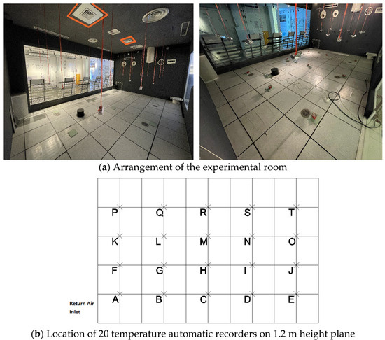
Figure 9.
Arrangement of the experimental room and the location of 20 temperature automatic recorders on 1.2 m height plane.
The preparation before the experiment consisted of four parts and equipment information is listed in Table 5:
Table 5.
Equipment information.
- 1.
- A balanced flow meter (TSI8380, Product of TSI from Dallas, TX, USA) was used to determine the supply airflow of the diffuser, the opening of the air valve, and the operating frequency of the fan. Before the experiment, error calibration of the instrument was carried out by official calibration organizations. The measured data show that when the supply airflow of two diffusers was 213 m3·h−1/per, the fan frequency was 35 Hz; when the supply airflow of two diffusers was 295 m3·h−1/per, the fan frequency was 46 Hz.
- 2.
- A three-phase electric power recorder (Fluke1735,Product of Fluke from Everett, WA, USA) was used to measure the electric power of each electric stove, and electric stoves with a power of between 195 W and 205 W were selected to ensure the uniform distribution of the indoor heat source. In addition, the total power of all electric stoves was monitored during the experiment to ensure the stability of the indoor heat source. As with the balanced flow meter, error calibration of the instrument was carried out by official calibration organizations before the experiment.
- 3.
- The experimental room was maintained at a positive pressure of about 1 Pa by adjusting the area of return air outlet, and the indoor and outdoor differential pressure was monitored during the experiment with a differential pressure meter (TSI 8345), so a stable amount of supply air flow and return air flow was ensured.
- 4.
- The error calibration of the temperature automatic recorder (Testo 174 H) was carried out before the experiment. All temperature automatic recorders were placed in the same place for 5 min, and the average temperature of all temperature automatic recorders was calculated as the real temperature of the environment, so the error of each temperature automatic recorder could be obtained. Table 6 lists the instrumentation errors of each temperature sensor.
Table 6.
Instrumentation errors of each temperature sensor (°C).
Table 6.
Instrumentation errors of each temperature sensor (°C).
| Temp. Sensor | A | B | C | D | E | F | G | H | I | J |
| Instrument Error | 0.1 | 0 | −0.5 | 0.2 | 0.2 | 0 | 0 | 0 | 0.2 | 0.1 |
| Temp. Sensor | K | L | M | N | O | P | Q | R | S | T |
| Instrument Error | −0.3 | 0 | −0.4 | 0.2 | 0.2 | 0 | −0.5 | 0 | 0.2 | 0.2 |
With different load distributions of the indoor electric stoves, and different supply air flow rates of the diffuser and size of return air inlet, three experimental scenarios were designed, as shown in Table 7. There were 9 electric stoves located according to plan_1 in Scenarios 1 and 2 and 15 electric stoves were located according to plan_2 in Scenario 3.
Table 7.
Parameters of three experimental scenarios.
Table 7.
Parameters of three experimental scenarios.
| Scenario | Internal Load (kW) | Total Air Flowrate in Room (m3·h−1) | Indoor Positive Pressure (Pa) | Size of Return Air Inlet (mm × mm) | |
|---|---|---|---|---|---|
| Scenario _1 | 1.95 (Electric stove location plan_1) | 426 | 2 | 215 × 160 | |
| Scenario _2 | 1.95 (Electric stove location plan_1) | 590 | 2 | 215 × 160 | |
| Scenario _3 | 3.25 (Electric stove location plan_2) | 590 | 1 | 215 × 220 | |
| Electric stove location plan_1 | Electric stove location plan_2 | ||||
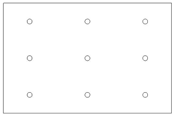 |  | ||||
3. Results and Discussion
3.1. Comparison and Discussion of Simulation and Experimental Results
The simulation results of the three experimental scenarios are shown in Table 8. The internal loads of Scenario 1 and Scenario 2 were the same, but the air supply volume of Scenario 2 was slightly larger than that of Scenario 1. Based on the principle of energy conservation, the indoor average temperature and the temperature at the height of 1.2 m working surface of Scenario 2 were slightly lower than that of Scenario 1. Scenario 2 and Scenario 3 had the same amount of air supply, but the internal load of Scenario 3 was larger than that of Scenario 2, so the average indoor temperature and the temperature at the height of 1.2 m working surface of Scenario 3 were higher than that of Scenario 2.
Table 8.
Simulation results of three experimental scenarios.
The temperature of the supply air was 18.5 °C throughout the experiment, and the ambient temperature was 21.3 °C. Each experimental scenario reached stability in about 3 h. The data of the temperature automatic recorders were collected and corrected based on errors after the experiment.
The indoor temperature distribution of each scenario could be obtained after the error correction. As shown in Figure 10, the simulated temperature distribution of the 20 points at the height of the 1.2 m working surface was quite consistent with the measured ones for the three scenarios, whose deviations were between −7.4~1.7%. In addition, the root mean square error of temperature for the three scenarios was 0.7 °C, 0.7 °C, and 1.0 °C, respectively. But the error was overall negative, and the simulation temperature was lower than the measured temperature. The possible reason was that instrument error of the balanced flow meter made the actual air volume smaller and the indoor temperature higher.
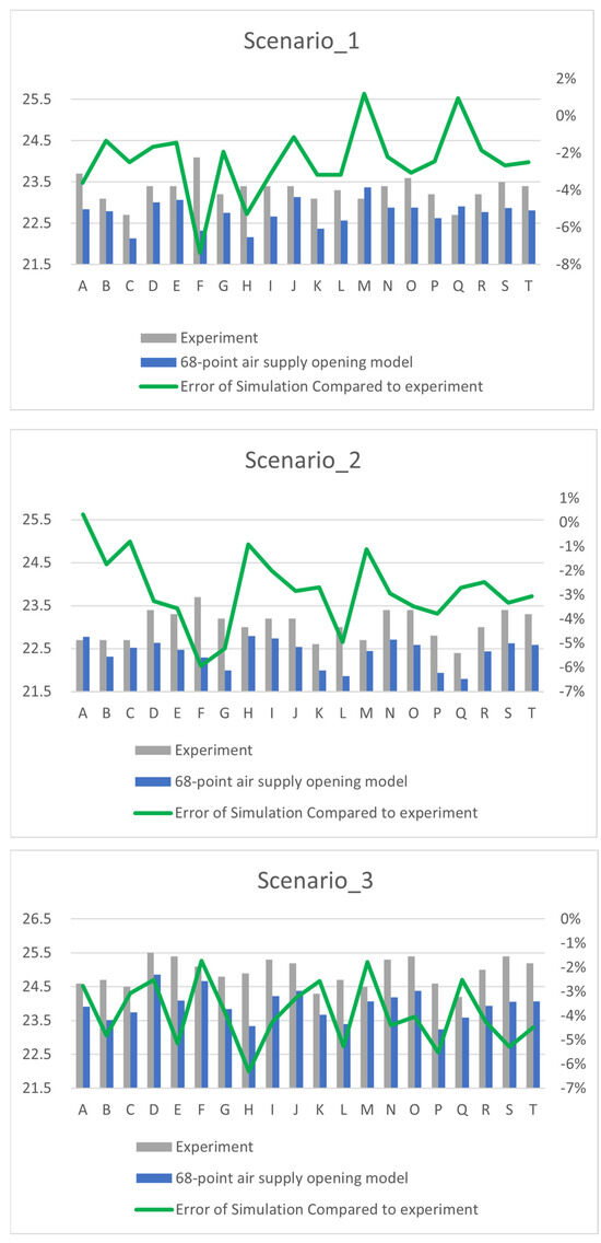
Figure 10.
Error comparison of measurement temperature at 1.2 m working surface height.
3.2. Analysis of Simulation Results
As the 68-point air supply opening model can effectively simplify the modelling of the diffuser, the non-uniform temperature distribution in the room can be accurately reflected from the simulation results. Figure 11 shows the simulation results of temperature distribution at the 1.2 m working surface height for the three experimental scenarios. The indoor non-uniform temperature distribution is affected by the internal load and air supply volume obviously. The location and size of the return air outlet affects the airflow organization in the room and thus the non-uniform temperature distribution in the room. Figure 12 shows the simulation results of temperature distribution at the longitudinal section along the center of the diffusers for the three experimental scenarios. The advection effect of diffusers is well reflected in these simplified simulations. Meanwhile, the airflow from different diffusers has mutual influence before it reaches the working area; therefore, the temperature of one location is determined by the integrated air flowrate of the surrounding diffusers. That is, the non-uniform temperature distribution in the room should consider the combined effect of the airflow from different diffusers in the room.
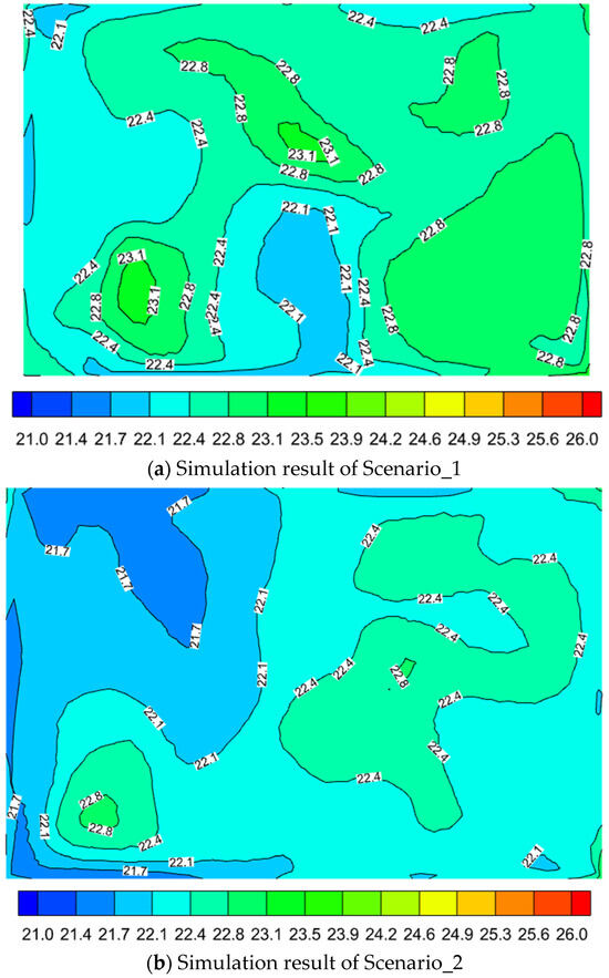
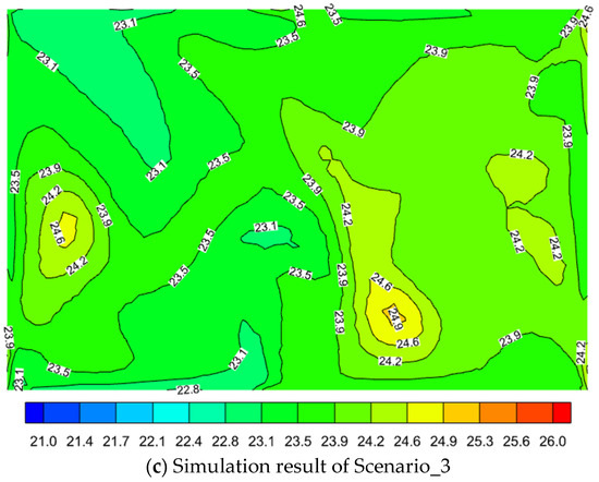
Figure 11.
Simulation results of temperature distribution at 1.2 m working surface height for three experimental scenarios (°C).
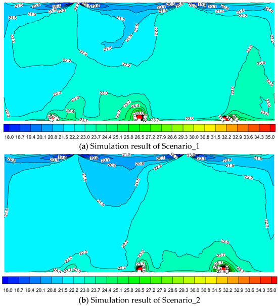
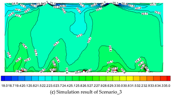
Figure 12.
Simulation results of temperature distribution at longitudinal section along the center of the diffusers for three experimental scenarios (°C).
Though the results were satisfactory, some limitations existed in the experiments. This paper investigated a simplified simulation method for four-way square diffusers. The experimental space was limited due to the diffuser type, with only two square diffusers installed. To better demonstrate the effectiveness of the simplified method for four-way square diffusers in simulating indoor non-uniform temperature distribution, it may be beneficial to choose a larger indoor space with more square diffusers for comparison with experimental results.
4. Conclusions
The contributions of this paper can be summarized as follows: (1) proposing a simplified CFD simulation method for four-way square diffusers, balancing the model complexity and the simulation accuracy; (2) demonstrating the mutual influence of the airflow from different diffusers; and (3) studying indoor non-uniform temperature distribution under the action of multiple diffusers.
A simulation of the airflow distribution on the outlet air supply cross-section of the four-way square diffuser was conducted. The diffuser outlet air supply cross-section was divided based on the airflow distribution characteristics and diffuser geometry. To simplify the diffuser, a 68-point air opening model was proposed and applied to simulate indoor non-uniform temperature distribution. Finally, the temperature distribution at a height of 1.2 m above the working surface in the room was obtained through CFD simulation and compared with experimental results. The results show that the simplified modeling of the diffuser using the 68-point air opening model can well simulate the influence of the diffuser outlet airflow distribution and the advection effect of diffusers. Comparing the simulation results with experiments, the deviations for the three scenarios werebetween −7.4~1.7% and the average deviation was −3.0%. Furthermore, the root mean square error of temperature for the three scenarios was 0.7 °C, 0.7 °C, and 1.0 °C, respectively. With the interaction of the airflow from adjacent diffusers, the temperature of one location is determined by the integrated air flowrate of the surrounding diffusers. That is, the non-uniform temperature distribution in the room should take into account the combined effect of the airflow from different diffusers in the room. Thus, an accurate indoor temperature distribution field can be obtained with the simplified modeling of the diffuser. Especially when there are multiple diffusers in the simulation room, the 68-point air-opening model can greatly reduce the modeling time and effectively simplify the model, which is a good way to balance the complexity of the model and the accuracy of the calculation.
Author Contributions
Conceptualization, Y.L. (Yuming Li), Y.P., Z.H. and X.Y.; methodology, Y.L. (Yuming Li), Y.P. and Z.H.; software, Y.L. (Yuming Li); validation, Y.L. (Yuming Li) and Y.L. (Yumin Liang); formal analysis, Y.L. (Yuming Li), Y.P. and Z.H.; investigation, Y.L. (Yuming Li) and Y.L. (Yumin Liang); resources, Y.L. (Yuming Li) and X.Y.; data curation, Y.L. (Yuming Li) and Y.L. (Yumin Liang); writing—original draft preparation, Y.L. (Yuming Li); writing—review and editing, Y.L. (Yuming Li), X.Y. and Y.L. (Yumin Liang); visualization, Y.L. (Yuming Li); supervision, Y.P. and Z.H.; project administration, Y.L. (Yuming Li), Y.P. and Z.H. All authors have read and agreed to the published version of the manuscript.
Funding
This research received no external funding.
Data Availability Statement
Data will be made available on request. The data are not publicly available due to privacy.
Conflicts of Interest
The authors declare no conflicts of interest. The funders had no role in the design of the study; in the collection, analyses, or interpretation of data; in the writing of the manuscript; or in the decision to publish the results.
References
- Lin, Y.; Huang, T.; Yang, W.; Hu, X.; Li, C. A Review on the Impact of Outdoor Environment on Indoor Thermal Environment. Buildings 2023, 13, 2600. [Google Scholar] [CrossRef]
- Liang, C.; Li, X.; Melikov, A.; Shao, X.; Li, B. A quantitative relationship between heat gain and local cooling load in a general non-uniform indoor environment. Energy 2019, 182, 412–423. [Google Scholar] [CrossRef]
- Li, Y.; Pan, Y.; Huang, Z.; Fu, L.; Li, J.; Sun, T.; Zhu, M.; Yuan, X. Numerical modeling of non-uniform indoor temperature distribution for coordinated air flow control. J. Build. Eng. 2024, 82, 108246. [Google Scholar] [CrossRef]
- Kong, M.; Dang, T.; Zhang, J.; Khalifa, H. Micro-environmental control for efficient local heating: CFD simulation and manikin test verification. Build. Environ. 2019, 147, 382–396. [Google Scholar] [CrossRef]
- Bresa, A.; Žakula, T.; Ajduković, D. Occupant preferences on the interaction with human-centered control systems in school buildings. J. Build. Eng. 2022, 64, 105489. [Google Scholar] [CrossRef]
- ISO Standard 7730 Ergonomics of the Thermal Environment; Analytical determination and Interpretation of Thermal Comfort Using Calculation of the PMV and PPD Indices and Local Thermal Comfort Criteria. International Standards Organization: Geneva, Switzerland, 2005.
- Su, X.; Yuan, Y.; Wang, Z.; Liu, W.; Lan, L.; Lian, Z. Human thermal comfort in non-uniform thermal environments: A review. Energy Built Environ. 2023, in press. [Google Scholar]
- ANSI/ASHRAE Standard 55-2013; Thermal Environmental Conditions for Human Occupancy. American Society of Heating, Refrigerating and Air-Conditioning Engineers Inc.: Atlanta, GA, USA, 2013.
- Gan, G. Analysis of mean radiant temperature and thermal comfort. Build. Serv. Eng. Res. Technol. 2001, 22, 95–101. [Google Scholar] [CrossRef]
- Zhang, S.; Cheng, Y.; Oladokun, M.; Huan, C.; Lin, Z. Heat removal efficiency of stratum ventilation for air-side modulation. Appl. Energy 2019, 238, 1237–1249. [Google Scholar] [CrossRef]
- Luo, Y.; Cui, D.; Song, Y.; Tian, Z.; Fan, J.; Zhang, L. Fast and accurate prediction of air temperature and velocity field in non-uniform indoor environment under complex boundaries. Build. Environ. 2023, 230, 109987. [Google Scholar] [CrossRef]
- Marek, B.; Marek, J.; Daniel, S.; Michał, K. Air flow characteristics of a room with air vortex diffuser. MATEC Web Conf. 2018, 240, 2002. [Google Scholar]
- Hurnik, M.; Kaczmarczyk, J.; Popiolek, Z. Study of Radial Wall Jets from Ceiling Diffusers at Variable Air Volume. Energies 2021, 14, 240. [Google Scholar] [CrossRef]
- Zhu, H.; Ren, C.; Cao, S. Fast prediction for multi-parameters (concentration, temperature and humidity) of indoor environment towards the online control of HVAC system. Build. Simul. 2021, 14, 649–665. [Google Scholar] [CrossRef]
- Dhahri, M.; Aouinet, H. CFD investigation of temperature distribution, air flow pattern and thermal comfort in natural ventilation of building using solar chimney. World J. Eng. 2020, 17, 78–86. [Google Scholar] [CrossRef]
- Aziz, M.; Gad, I.; Mohammed, E.; Mohammed, R. Experimental and numerical study of influence of air ceiling diffusers on room air flow characteristics. Energy Build. 2012, 55, 738–746. [Google Scholar] [CrossRef]
- Nocente, A.; Arslan, T.; Grynning, S.; Goia, F. CFD Study of Diffuse Ceiling Ventilation through Perforated Ceiling Panels. Energies 2020, 13, 1995. [Google Scholar] [CrossRef]
- Li, K.; Song, L.; Zhang, X.; Wang, Q.; Hua, J. Study of Influence of Boundary Condition of Diffuser with Non-Uniform Velocity on the Jet Characteristics and Indoor Flow Field. Energies 2023, 16, 1079. [Google Scholar] [CrossRef]
- Izadyar, N.; Miller, W.; Rismanchi, B.; Hansen, V. Numerical simulation of single-sided natural ventilation: Impacts of balconies opening and depth scale on indoor environment. IOP Conf. Ser. Earth Environ. Sci. 2020, 463, 012037. [Google Scholar] [CrossRef]
- Zhao, W.; Ye, W.; Zhang, Q.; Zhang, X. Simulations on arrangements of induced jet-fans as auxiliary ventilation for a mechanical ventilated space with openings. E3S Web Conf. 2019, 111, 01036. [Google Scholar] [CrossRef]
- Mou, J.; Cui, S.; Khoo, D. Computational fluid dynamics modelling of airflow and carbon dioxide distribution inside a seminar room for sensor placement. Meas. Sens. 2022, 23, 100402. [Google Scholar] [CrossRef]
- Liu, Y.; Long, Z.; Liu, W. A semi-empirical mesh strategy for CFD simulation of indoor airflow. Indoor Built Environ. 2022, 31, 2240–2256. [Google Scholar] [CrossRef]
- Wang, F.; Zhou, X.; Kikumoto, H. Improvement of optimization methods in indoor time-variant source parameters estimation combining unsteady adjoint equations and flow field information. Build. Environ. 2022, 226, 109710. [Google Scholar] [CrossRef]
- Turek, V. Improving Performance of Simplified Computational Fluid Dynamics Models via Symmetric Successive Overrelaxation. Energies 2019, 12, 2438. [Google Scholar] [CrossRef]
- Nielsen, P. Description of Supply Openings in Numerical Models for Room Air Distribution. ASHRAE Transactions; Aalborg University: Aalborg, Denmark, 1992; Volume 98. [Google Scholar]
- Srebric, J.; Chen, Q. Simplified numerical models for complex air supply diffusers. HVACR Res. 2002, 8, 277–294. [Google Scholar] [CrossRef]
- Li, X.; Zhao, B.; Guan, P.; Ren, H. Air Supply Opening Model of Ceiling Diffusers for Numerical Simulation of Indoor Air Distribution under Actual Connected Conditions, Part II: Application of the Model. Numer. Heat Transf. Part Appl. 2006, 49, 821–830. [Google Scholar] [CrossRef]
- Abdelmaksoud, W. Simplified CFD Model for Perforated Tile with Distorted Outflow. Fluids 2022, 7, 112. [Google Scholar] [CrossRef]
- Luca, B.; Lorenzo, M.; Massimiliano, R.; Prisco, P.; Alessandro, M.; Aurelio, S. The Role of Air Conditioning in the Diffusion of Sars-CoV-2 in Indoor Environments: A First Computational Fluid Dynamic Model, based on Investigations performed at the Vatican State Children’s Hospital. Environ. Res. 2021, 193, 110343. [Google Scholar]
- Jaszczur, M.; Madejski, P.; Kleszcz, S.; Zych, M.; Palej, P. Numerical and experimental analysis of the air stream generated by square ceiling diffusers. E3S Web Conf. 2019, 128, 08003. [Google Scholar] [CrossRef]
- Wu, W.; Yoon, N.; Tong, Z.; Chen, Y.; Lv, Y.; Arenlund, T.; Benner, J. Diffuse ceiling ventilation for buildings: A review of fundamental theories and research methodologies. J. Clean. Prod. 2019, 211, 1600–1619. [Google Scholar] [CrossRef]
- Ansys Fluent Theory Guide; ANSYS Inc.: Canonsburg, PA, USA, 2020.
- Argyropoulosa, C.; Markatos, N. Recent advances on the numerical modelling of turbulent flows. Appl. Math. Model. 2015, 39, 693–732. [Google Scholar] [CrossRef]
- Pope, S. Turbulent Flows; Cambridge University Press: Cambridge, UK, 2001; pp. 358–385. [Google Scholar]
- Yang, X.; Zhang, Y.; Hang, J.; Lin, Y.; Mattsson, M.; Sandberg, M.; Zhang, M.; Wang, K. Integrated assessment of indoor and outdoor ventilation in street canyons with naturally-ventilated buildings by various ventilation indexes. Build. Environ. 2020, 169, 106528. [Google Scholar] [CrossRef]
- Mahdi, A.; Alamir, Q.; Yakoob, A. Air Distribution Performance Inside Office Room with Combined Displacement and Personal Ventilation. IOP Conf. Ser. Mater. Sci. Eng. 2020, 978, 012048. [Google Scholar] [CrossRef]
Disclaimer/Publisher’s Note: The statements, opinions and data contained in all publications are solely those of the individual author(s) and contributor(s) and not of MDPI and/or the editor(s). MDPI and/or the editor(s) disclaim responsibility for any injury to people or property resulting from any ideas, methods, instructions or products referred to in the content. |
© 2024 by the authors. Licensee MDPI, Basel, Switzerland. This article is an open access article distributed under the terms and conditions of the Creative Commons Attribution (CC BY) license (https://creativecommons.org/licenses/by/4.0/).