
Deflection Monitoring Method for Simply Supported Girder Bridges Using Strain Response under Traffic Loads


Abstract
:1. Introduction
2. Theory of Deflection Calculation Based on Strain Measurement Input
2.1. Deflection Calculation Based on Distributed Strain Measurement Input
2.2. Assessment Method of Deflection Based on Strain Measurements at One Location under TrafficLoad
2.2.1. Displacement Reciprocal Theorem
2.2.2. Static Strain Distribution Obtained with One Strain Sensor under Traffic Loads
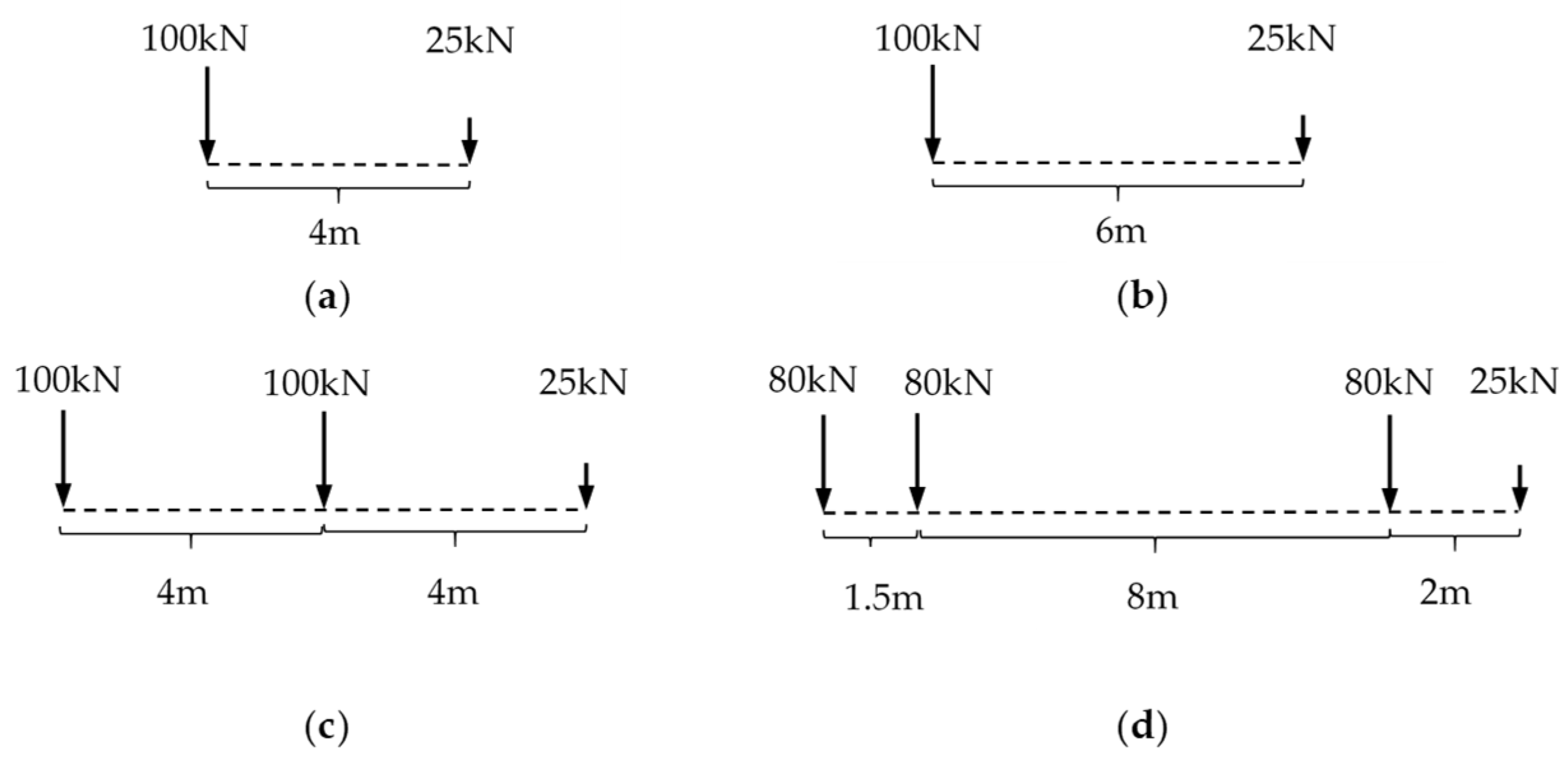
- (1)
- Uniaxial vehicle load
- (2)
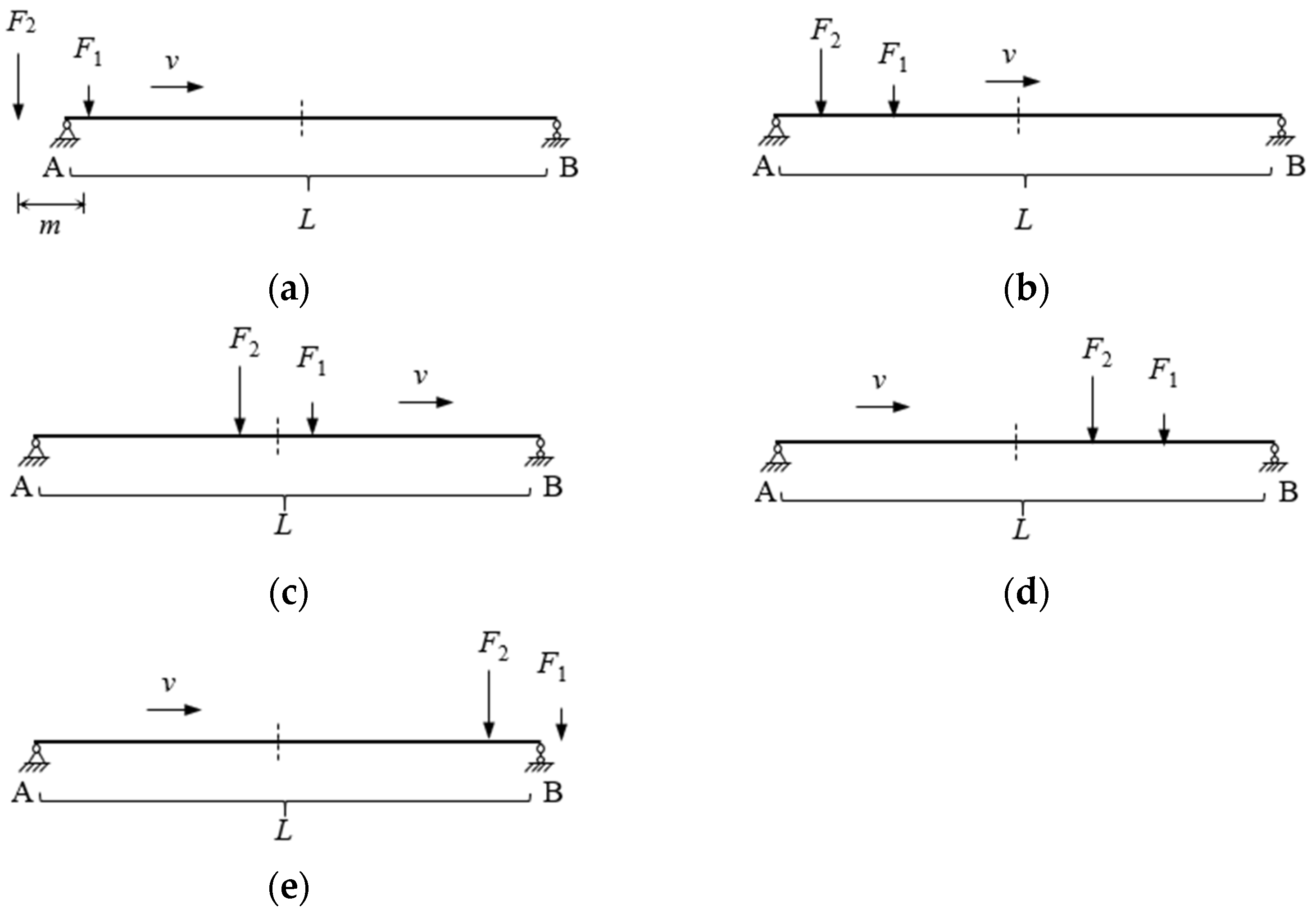
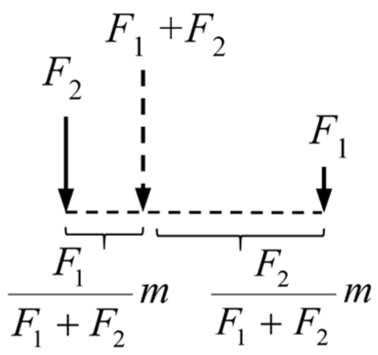
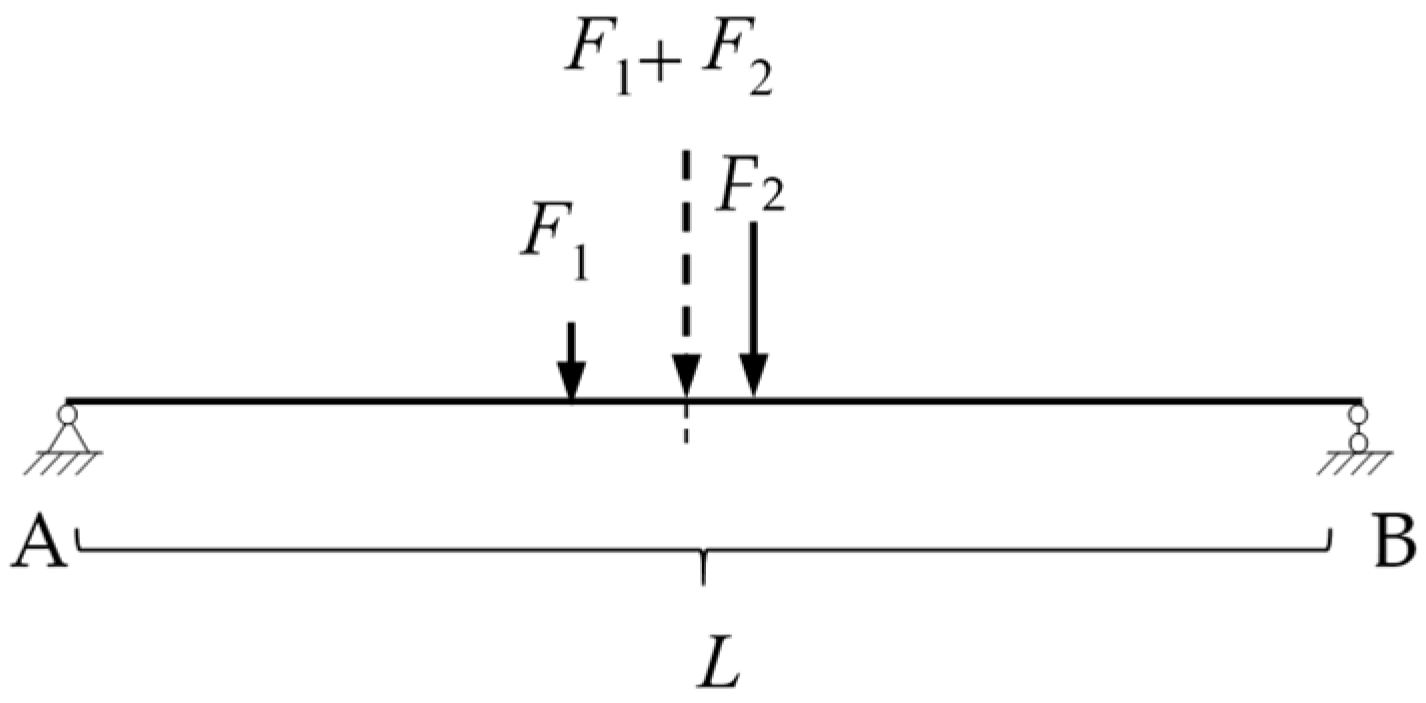
- Biaxial vehicle load
- (3)
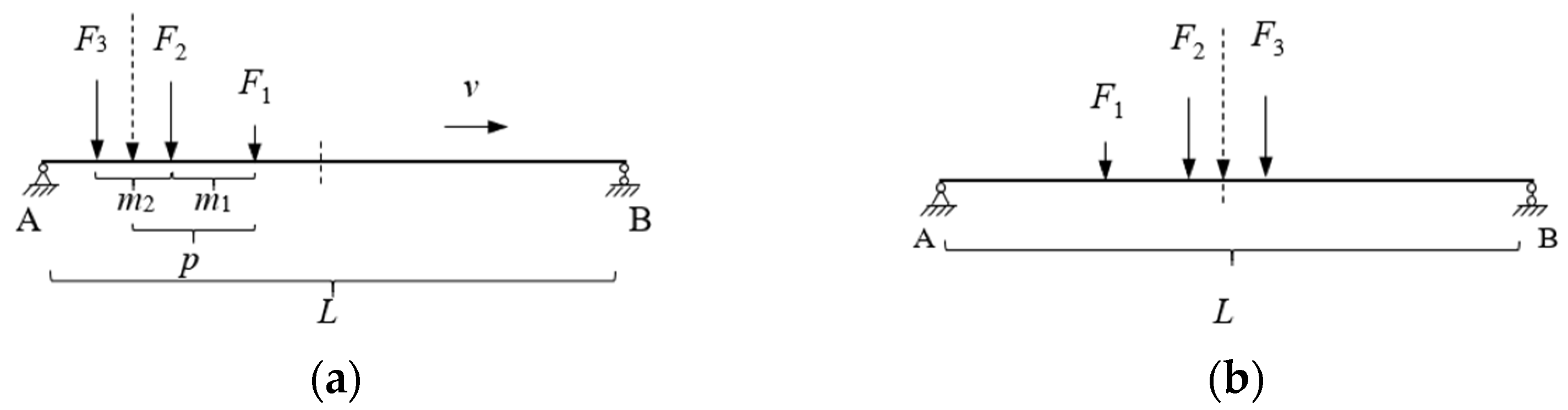
- Multi-axle vehicle load
3. Strain Measurement Based on Optical Fibre Sensors
3.1. Strain Measurement Principle
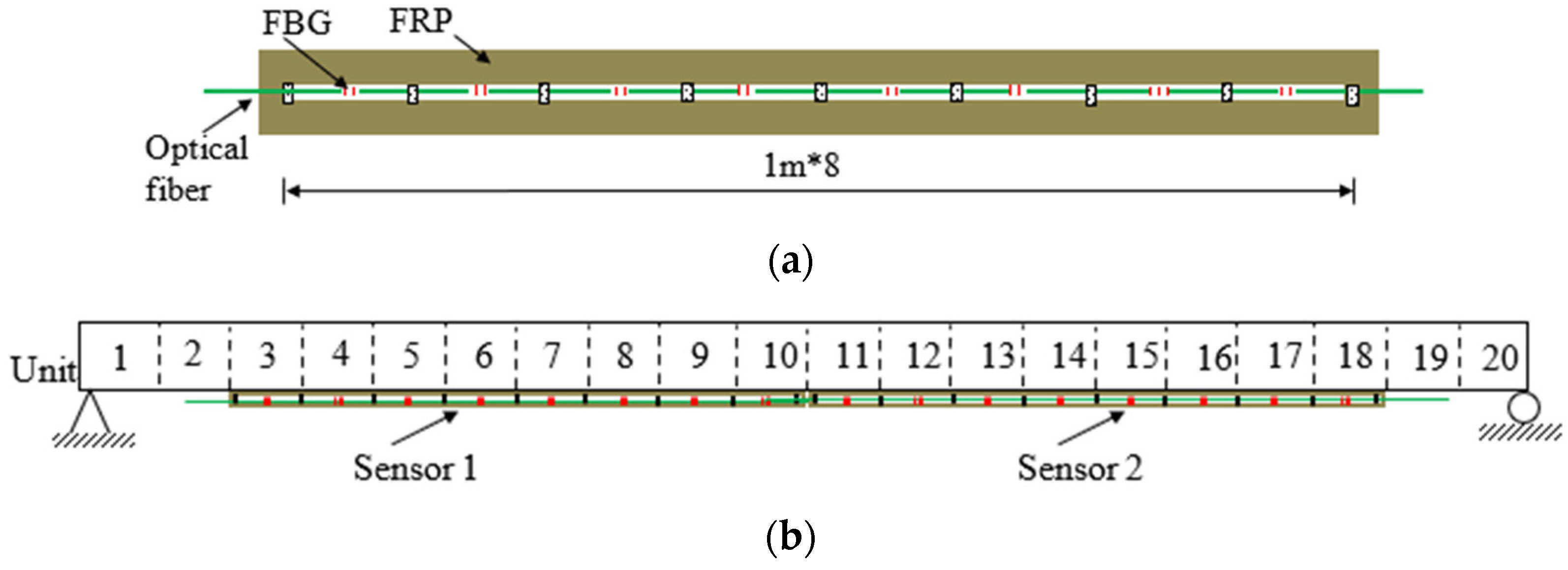
3.2. Long-Gauge Optical Fibre Sensor
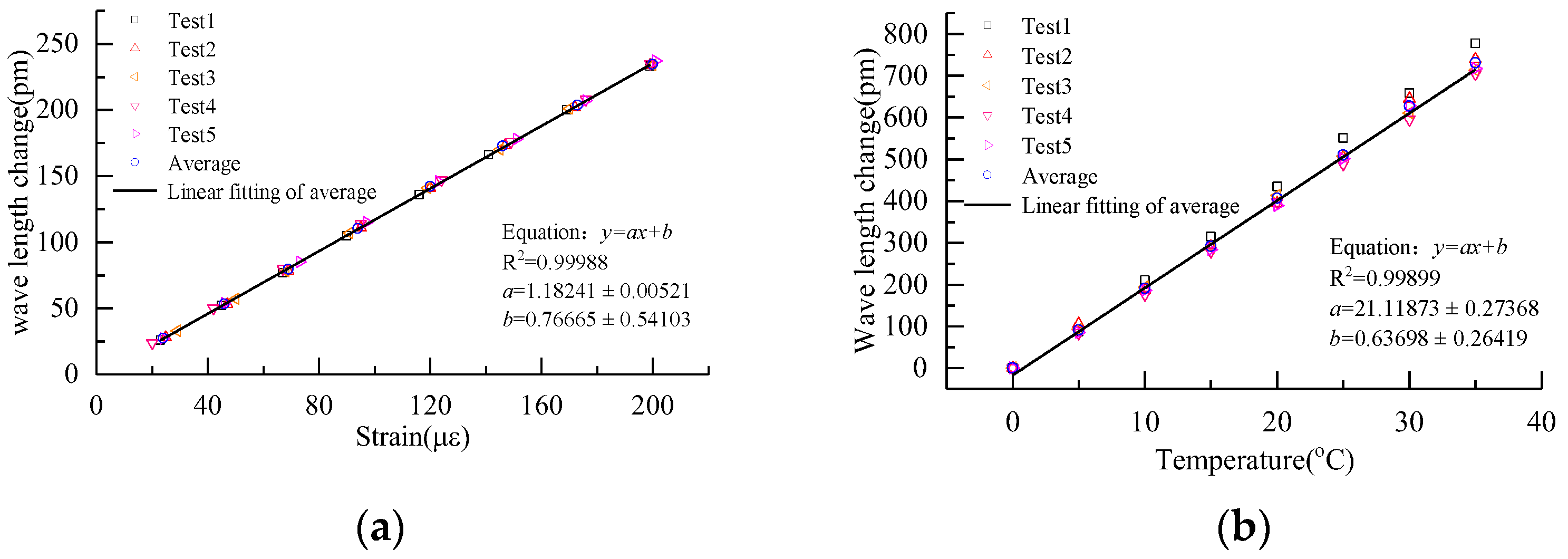
3.3. Strain Sensing Performance of the Sensor
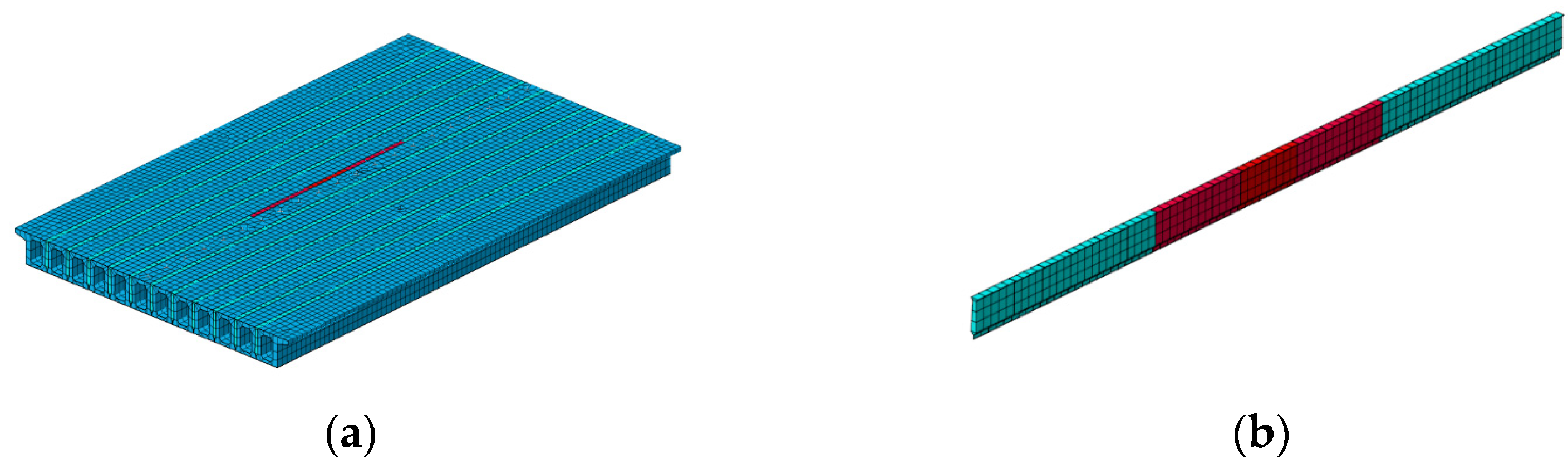
4. Study on the FE Bridge Model
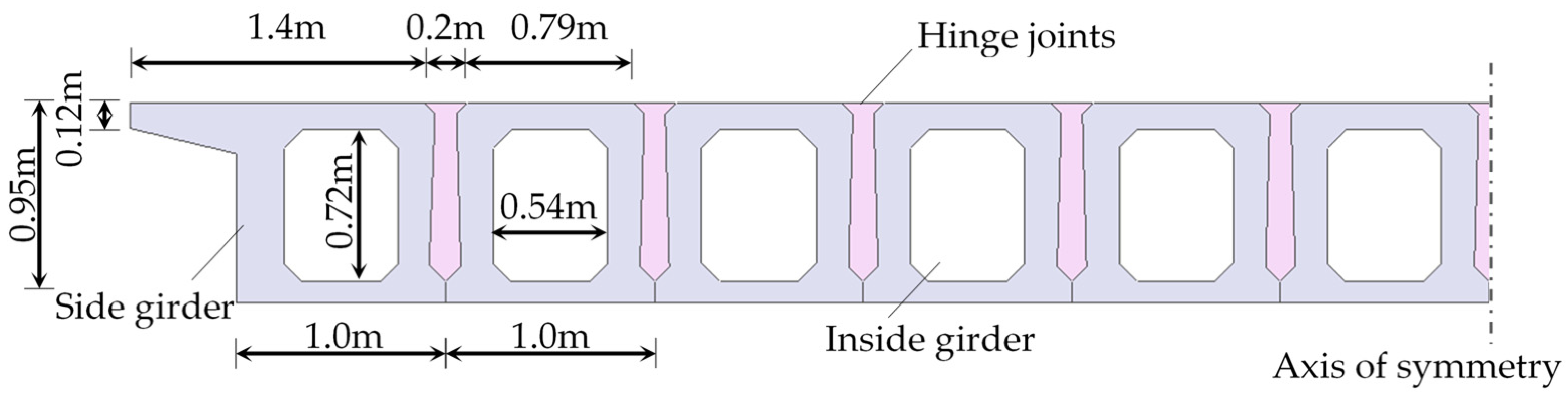
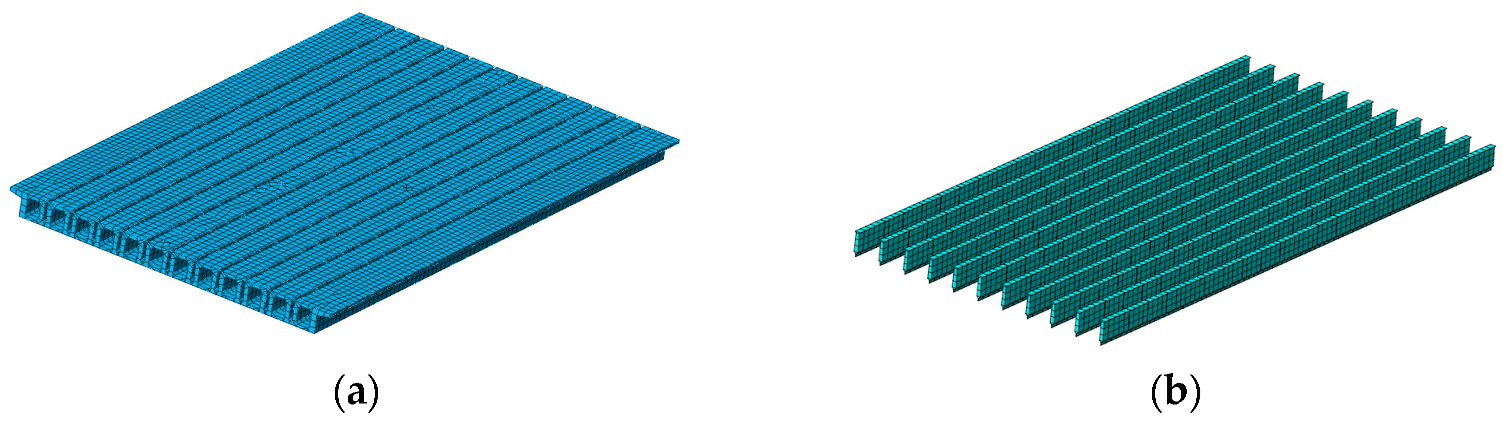
4.1. Introduction to the Bridge Model
4.2. Extraction and Processing of Strain Data
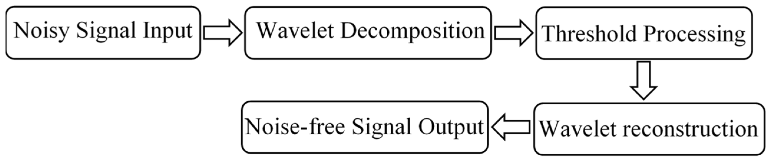
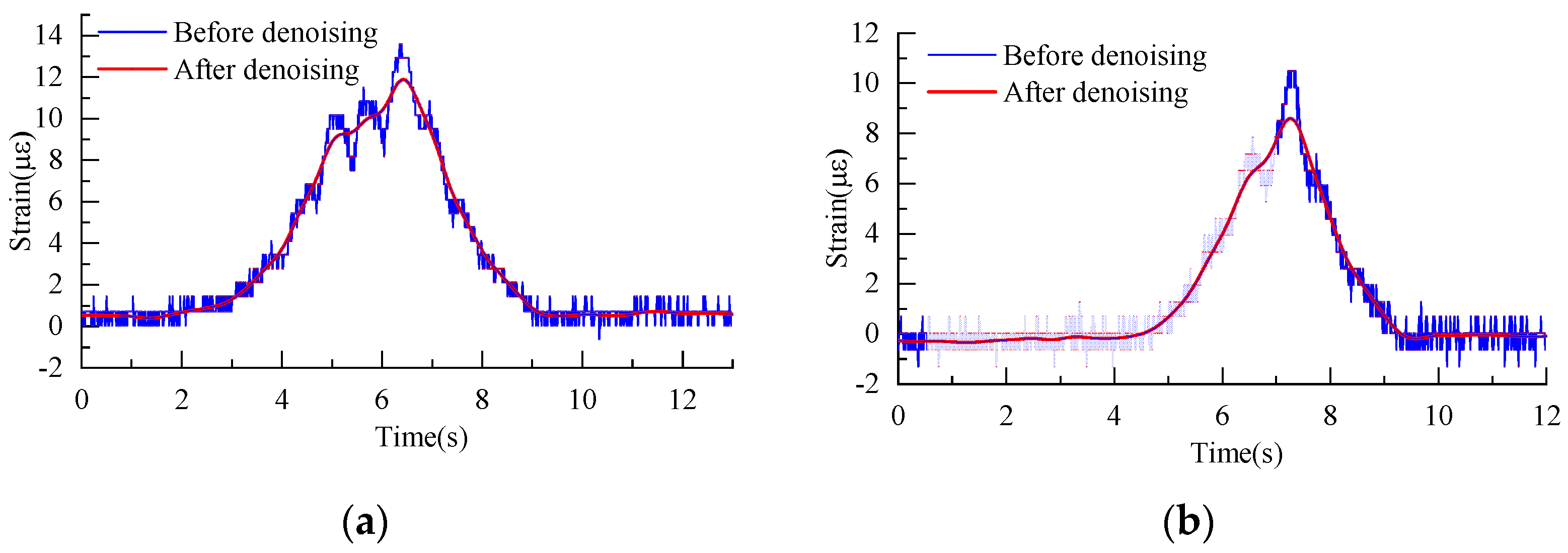
- Wavelet decomposition. Generally, a wavelet basis type and the layer N of wavelet decomposition are selected first, and then N layer decomposition of the noisy signal is performed to obtain the wavelet coefficient of each layer. The wavelet basis function used in this paper is Sym8, which has already been used in many application scenarios in signal processing and data compression. Sym8 can decompose the data signal into multiple sub-signals, reducing the data noise while retaining the important features of the signal. It can retain the important features of the signal as much as possible and remove the noise interference. Here N is set as 4.
- Threshold processing. The wavelet coefficients from the first layer to the N layer are processed with appropriate thresholds, and the noise is removed with its de-correlation (Figure 15). The main principle is to set a threshold λ. When the wavelet coefficient is greater than λ, it retains its original value. When the wavelet coefficient is less than λ, it is directly set to 0. In this way, the original features are well preserved and the noise removal signal is smoother.
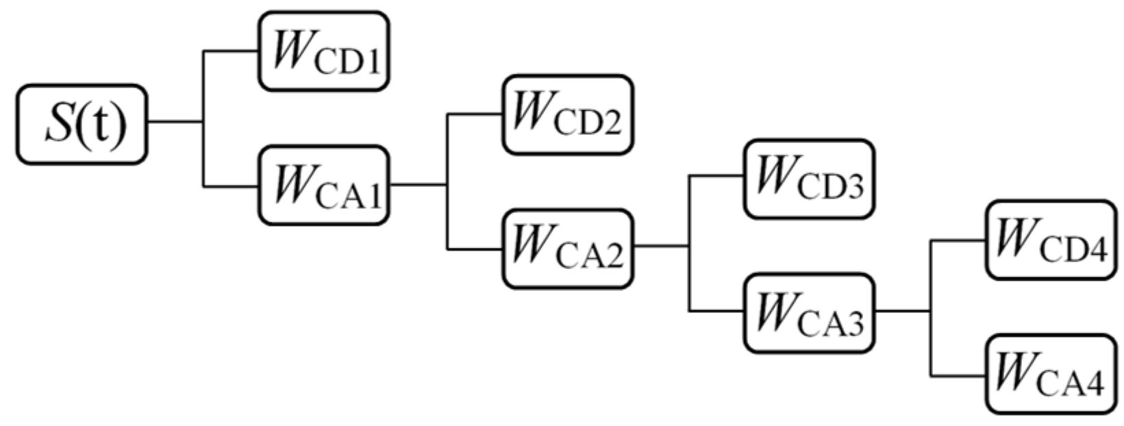
- Wavelet reconstruction. The processed signal is reconstructed and the denoised signal is obtained. In Figure 16, the signal S(t) is decomposed by four-layer wavelet, in which WCD1, WCD2, WCD3, and WCD4 are the high-frequency wavelet coefficients of each layer wavelet decomposition, while WCA1, WCA2, WCA3, and WCA4 are the low-frequency wavelet coefficients. Here, noise is mainly contained in the low-frequency wavelet coefficient, so it is considered that WCA1, WCA2, WCA3, and WCA4 are less than λ, and then can be set as 0. Finally, the denoised signal is obtained.
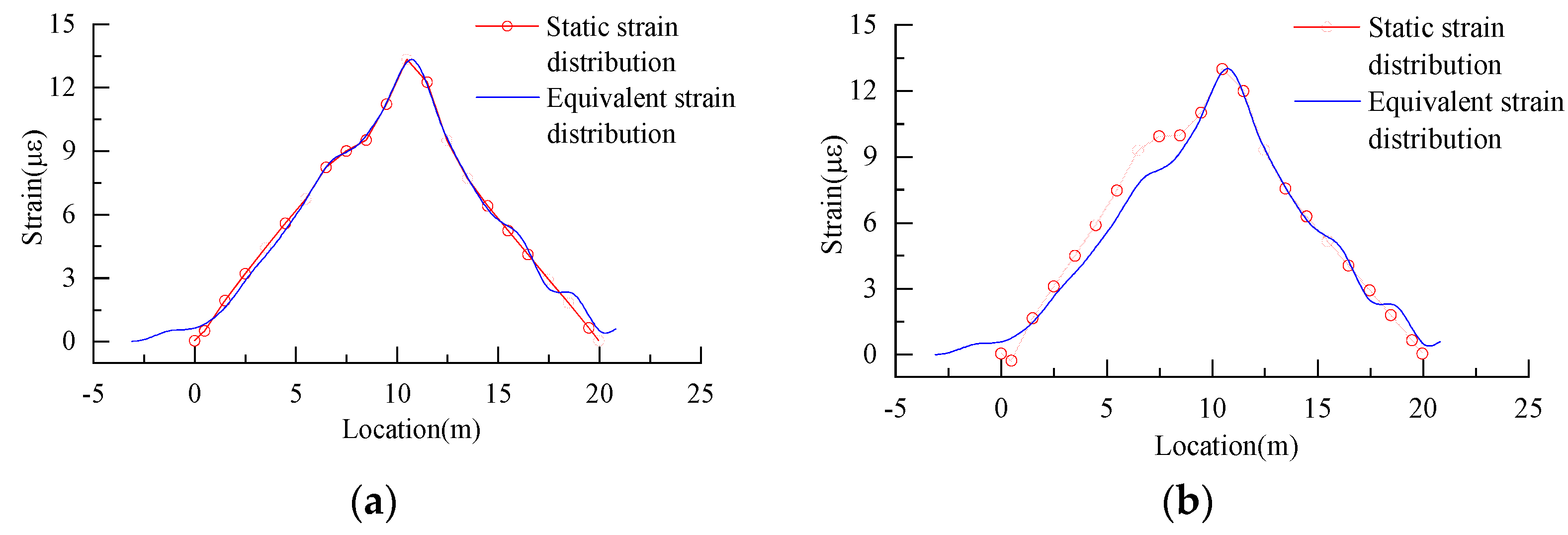
4.3. Results and Analysis
4.4. Parameter Influence Analysis
- (1)
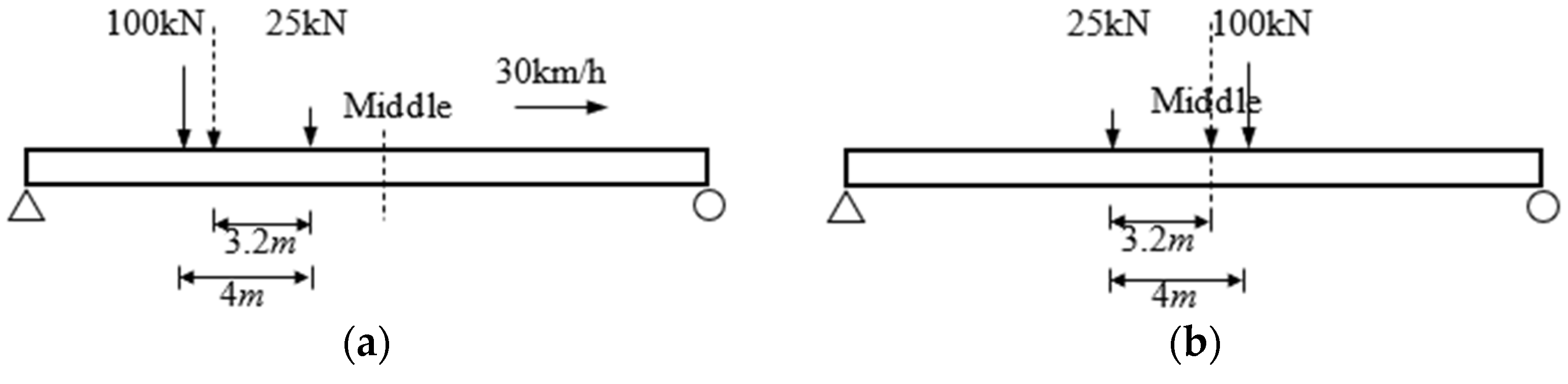
- Vehicle type
- (2)
- Vehicle speed
- (3)
- Structural damage
- (1)
- Damage between the hinge joints
- (2)
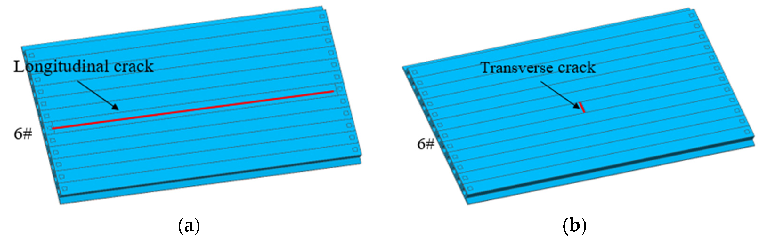
- Concrete cracks
5. On-Site Experimental Study
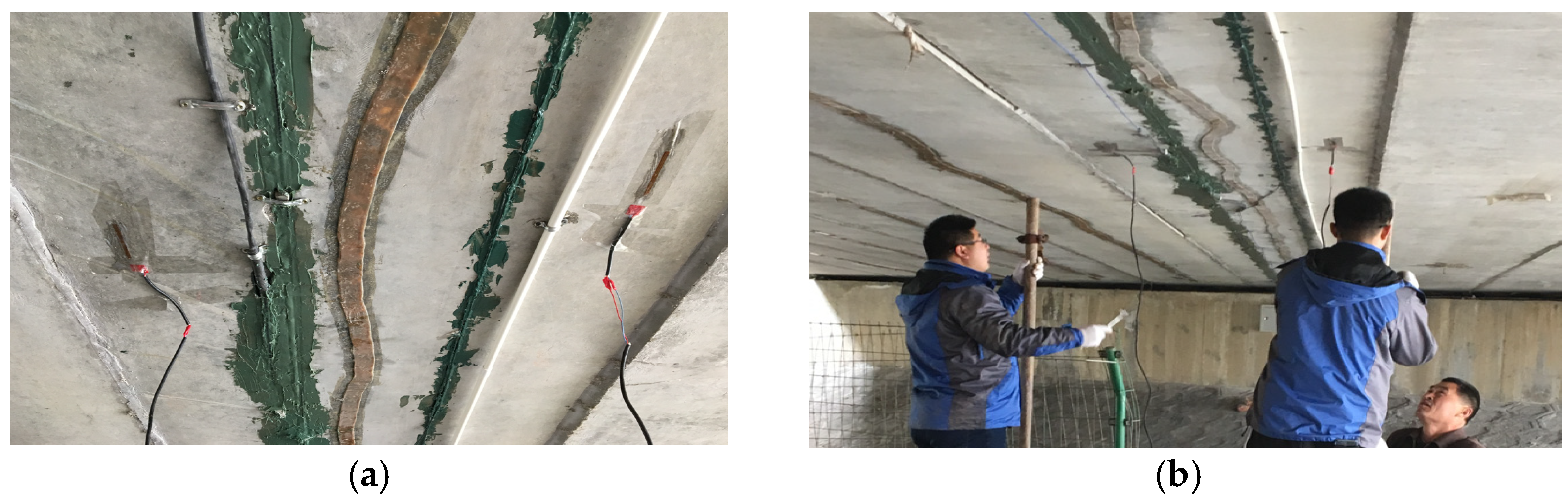
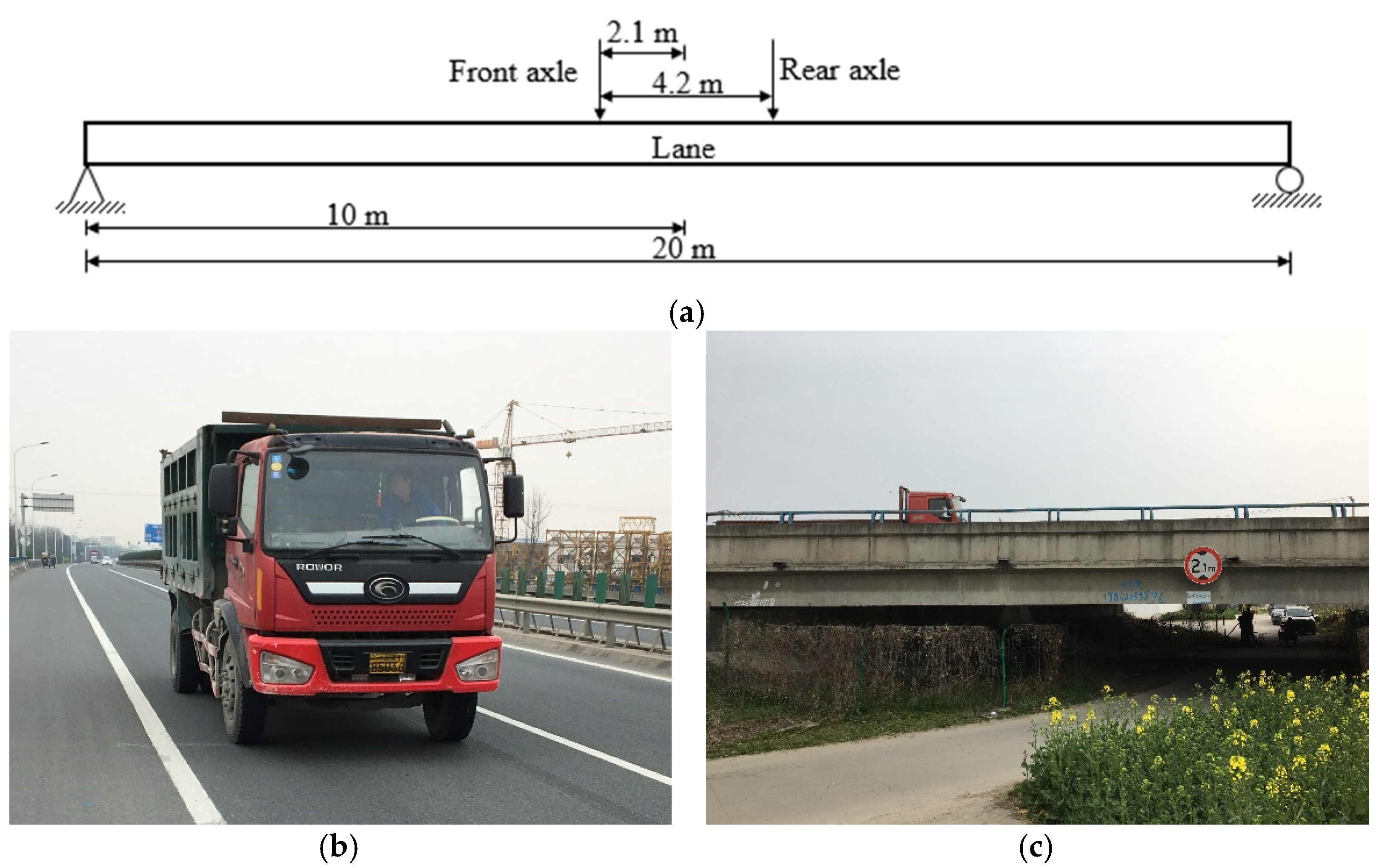
5.1. Experimental Description
5.2. Experimental Results and Analysis
6. Conclusions and Remarks
- (1)
- The displacement reciprocal theorem enabled the development of a method for converting the temporal strain response under traffic loads to the spatial distribution of strain under the same static loads. Meanwhile, modified methods for decreasing the error caused by vehicle type differences were established.
- (2)
- The deflection measurement method relied largely on strain distribution input, which was measured using the proposed macro-strain sensor, a long-gauge FBG sensor. The high accuracy of the proposed method was validated by FE simulation results, which indicated a relative error of about 5%. However, when key parameters such as vehicle type, vehicle speed, and structural damage were considered, damage to the hinge joint in the middle location significantly affected the proposed method’s accuracy, as the deflection error could exceed 10%.
- (3)
- The results of on-site experiments validated the proposed method, as the maximum relative error of deflection measurement was about 8% and the absolute error was below 0.05 mm.
Author Contributions
Funding
Data Availability Statement
Conflicts of Interest
References
- Yang, D.H.; Zhou, H.; Yi, T.H.; Li, H.N.; Bai, H.F. Joint deterioration detection based on field-identified lateral deflection influence lines for adjacent box girder bridges. Struct. Control Health Monit. 2022, 29, e3053. [Google Scholar] [CrossRef]
- Cusson, D.; Lounis, Z.; Daigle, L. Durability monitoring for improved service life predictions of concrete bridge decks in corrosive environments. Comput. Aided Civ. Infrastruct. Eng. 2011, 26, 524–541. [Google Scholar] [CrossRef]
- Wen, X.L.; Wei, L.; Dan, D.H.; Liu, G.M. Study on a measurement index of transverse collaborative working performance of prefabricated girder bridges. Adv. Struct. Eng. 2017, 20, 1879–1890. [Google Scholar] [CrossRef]
- Zhang, L.; Feng, D.M.; Wu, G. Simultaneous identification of bridge damage and vehicle parameters based on bridge strain responses. Struct. Control Health Monit. 2022, 29, e2945. [Google Scholar] [CrossRef]
- Daniel, M.; Abdollah, M.; Eugene, O.B. Bridge health monitoring using deflection measurements under random traffic. Struct. Control Health Monit. 2020, 27, e2593. [Google Scholar]
- Zhu Ge, S.; Xu, X.P.; Zhong, L.J.; Gan, S.W.; Lin, B.; Yang, X.; Zhang, X.H. Noncontact deflection measurement for bridge through a multi-UAVs system. Comput. Aided Civ. Infrastruct. Eng. 2021, 37, 746–761. [Google Scholar] [CrossRef]
- Jacek, K.; Wojciech, A.; Damian, B. Comparison of non-destructive techniques for technological bridge deflection testing. Materials 2020, 13, e1908. [Google Scholar]
- Oleksandr, P.M.; Oleksandr, M.S.; Yaroslav, L.I.; Petro, S.K. Multilaser spot tracking technology for bridge structure displacement measuring. Struct. Control Health Monit. 2021, 28, e2675. [Google Scholar]
- Erdoğan, H.; Gülal, E. Ambient Vibration Measurements of the Bosphorus Suspension Bridge by Total Station and GPS. Struct. Control Health Monit. 2013, 37, 16–23. [Google Scholar] [CrossRef]
- Pan, X.D.; Zhao, L. Laboratory experiment study on real-time monitoring and safety early warning system of structure settlement and deformation. Appl. Mech. Mater. 2015, 775, 264–267. [Google Scholar] [CrossRef]
- Lee, Z.K.; Bonopera, M.; Hsu, C.C.; Lee, B.H.; Yeh, F.Y. Long-term deflection monitoring of a box girder bridge with an optical-fibre, liquid-level system. Structures 2022, 44, 904–919. [Google Scholar] [CrossRef]
- Santhosh, K.V.; Roy, B.K. Online implementation of an adaptive calibration technique for displacement measurement using LVDT. Appl. Soft Comput. 2017, 53, 19–26. [Google Scholar]
- Sarthak, J.; Shrikant, M.H. Linear variable differential transducer (LVDT) & its applications in civil engineering. Int. J. Transp. Eng. Technol. 2017, 3, 62–66. [Google Scholar]
- Xu, Y.; James, M.W.B.; David, H.; Koo, K.Y. Long-span bridges: Enhanced data fusion of GPS displacement and deck accelerations. Eng. Struct. 2017, 147, 639–651. [Google Scholar] [CrossRef]
- GEsteban, V.B.; JRamon, G.C.; Rick, B.; Michel, G.A.; Ivan, E.G.C. Structural evaluation of dynamic and semi-static displacements of the Juarez Bridge using GPS technology. Measurement 2017, 110, 146–153. [Google Scholar]
- Hussein, A.M.; Panos, A.P.; Craig, M.H.; Gethin, W.R.; Lukasz, B. Monitoring the response of Severn Suspension Bridge in the United Kingdom using multi-GNSS measurements. Struct. Control Health Monit. 2021, 28, e2830. [Google Scholar]
- Meng, X.; Dodson, A.H.; Roberts, G.W. Detecting bridge dynamics with GPS and triaxial accelerometers. Eng. Struct. 2007, 29, 3178–3184. [Google Scholar] [CrossRef]
- Rujika, T.; Punchet, T.; Said, E. CCTV camera array for the displacement and strain measurement of a beam specimen in a laboratory. Buildings 2022, 12, 1778. [Google Scholar]
- Francisco, B.; Susana, A.; Pedro, J.S.; António, C.; Paulo, J.T.; Pedro, M.G.P.M.; Ranzal, D.; Cardoso, N.; Fernandes, N.; Fernandes, R.; et al. Displacement monitoring of a pedestrian bridge using 3D digital image correlation. Procedia Struct. Integr. 2022, 37, 880–887. [Google Scholar]
- Marie, A.; Olivier, P.; Noémie, P.; Emile, R.; Pierre, V. In situ DIC method to determine stress state in reinforced concrete structures. Measurement 2023, 210, 112483. [Google Scholar]
- Sun, L.; Li, Y.X.; Zhang, W. Experimental study on continuous bridge-deflection estimation through inclination and strain. J. Bridge Eng. 2020, 25, e04020020. [Google Scholar] [CrossRef]
- Hong, W.; Qin, Z.; Lv, K.; Fang, X. An indirect method for monitoring dynamic deflection of beam-like structures based on strain responses. Appl. Sci. 2018, 8, e811. [Google Scholar] [CrossRef]
- Feng, X.; Sun, C.S.; Zhang, X.T.; Ansari, F. Determination of the coefficient of thermal expansion with embedded long-gauge fibre optic sensors. Meas. Sci. Technol. 2010, 21, e065302. [Google Scholar] [CrossRef]
- Tang, Y.S.; Wu, Z.S. Distributed long-gauge optical fibre sensors based self-sensing FRP bar for concrete structure. Sensors 2016, 16, 286–303. [Google Scholar] [CrossRef]
- Tang, Y.S.; Jiang, T.F.; Wan, Y. Structural monitoring method for RC column with distributed self-sensing BFRP bars. Case Stud. Constr. Mater. 2022, 17, e01616. [Google Scholar] [CrossRef]
- Tang, Y.S.; Cao, M.F.; Li, B.; Chen, X.H.; Wang, Z.Y. Horizontal Deformation Monitoring of Concrete Pile with FRP-Packaged Distributed Optical-Fibre Sensors. Buildings 2023, 13, 2454. [Google Scholar] [CrossRef]


| Elastic Mode for Girder | Compressive Strength for Girder | Tensile Strength for Girder | Elastic Mode for Joints | Compressive Strength for Joints | Tensile Strength for Girder |
|---|---|---|---|---|---|
| 32.5 GPa | 19.1 Mpa | 1.71 Mpa | 30 Gpa | 14.3 Mpa | 1.43 Mpa |
| Girder No. | Actual Deflection (mm) | Deflection by Static Strain Distribution | Deflection by Equivalent Strain Distribution | ||
|---|---|---|---|---|---|
| Deflection (mm) | Error (%) | Deflection (mm) | Error (%) | ||
| 1 | 0.83 | 0.86 | 3.39 | 0.88 | 5.63 |
| 2 | 0.83 | 0.85 | 2.61 | 0.86 | 3.34 |
| 3 | 0.85 | 0.85 | 0.00 | 0.85 | 0.62 |
| 4 | 0.85 | 0.85 | 0.00 | 0.86 | 0.84 |
| 5 | 0.86 | 0.86 | 0.00 | 0.86 | 0.11 |
| 6 | 0.86 | 0.86 | 0.00 | 0.86 | −0.05 |
| Vehicle Type | Actual Deflection (mm) | Deflection by Static Strain Distribution | Deflection by Equivalent Strain Distribution | ||
|---|---|---|---|---|---|
| Deflection (mm) | Error (%) | Deflection (mm) | Error (%) | ||
| Biaxial van | 0.86 | 0.86 | 0.00 | 0.86 | −0.03 |
| Biaxial truck | 0.81 | 0.82 | 1.12 | 0.82 | 1.92 |
| Three-axle truck | 1.44 | 1.46 | 1.35 | 1.45 | 0.81 |
| Multi-axle trailer | 1.40 | 1.40 | 0.00 | 1.32 | −5.62 |
| Item | Actual Deflection | Deflection by Static Strain Distribution | Deflection by Equivalent Strain Distribution | |||
|---|---|---|---|---|---|---|
| 30 km/h | 60 km/h | 90 km/h | 120 km/h | |||
| Deflection (mm) | 0.86 | 0.86 | 0.86 | 0.86 | 0.87 | 0.92 |
| Error (%) | / | 0.00 | −0.05 | 0.41 | 1.20 | 5.50 |
| D | Actual Deflection (mm) | Static Strain Distribution | Equivalent Strain Distribution | ||
|---|---|---|---|---|---|
| Deflection (mm) | Error (%) | Deflection (mm) | Error (%) | ||
| 0.1 | 0.86 | 0.87 | 0.66 | 1.00 | 15.88 |
| 0.2 | 0.89 | 0.89 | 0.01 | 1.02 | 15.37 |
| 0.3 | 0.92 | 0.92 | −0.70 | 1.09 | 17.63 |
| 0.4 | 0.97 | 0.95 | −1.45 | 1.14 | 17.60 |
| 0.5 | 1.02 | 1.00 | −2.24 | 1.18 | 15.97 |
| 0.6 | 1.08 | 1.04 | −3.11 | 1.22 | 13.53 |
| 0.7 | 1.14 | 1.10 | −4.06 | 1.26 | 10.46 |
| 0.8 | 1.22 | 1.16 | −5.14 | 1.30 | 6.91 |
| 0.9 | 1.31 | 1.23 | −6.34 | 1.35 | 2.78 |
| 1.0 | 1.76 | 1.65 | −6.33 | 1.66 | −5.78 |
| D | Actual Deflection (mm) | Static Strain Distribution | Equivalent Strain Distribution | ||
|---|---|---|---|---|---|
| Deflection (mm) | Error (%) | Deflection (mm) | Error (%) | ||
| 0.05 | 0.87 | 0.88 | 1.12 | 0.88 | 1.54 |
| 0.10 | 0.87 | 0.88 | 1.10 | 0.88 | 1.51 |
| 0.15 | 0.87 | 0.88 | 1.07 | 0.88 | 1.42 |
| 0.20 | 0.87 | 0.88 | 1.04 | 0.88 | 1.27 |
| 0.25 | 0.87 | 0.88 | 1.00 | 0.88 | 0.94 |
| 0.30 | 0.87 | 0.88 | 0.96 | 0.87 | 0.36 |
| 0.35 | 0.87 | 0.88 | 0.95 | 0.86 | −0.60 |
| 0.40 | 0.87 | 0.88 | 1.00 | 0.85 | −2.18 |
| 0.45 | 0.88 | 0.89 | 1.13 | 0.84 | −4.05 |
| Condition | Actual Deflection (mm) | Static Strain Distribution | Equivalent Strain Distribution | ||
|---|---|---|---|---|---|
| Deflection (mm) | Error (%) | Deflection (mm) | Error (%) | ||
| Longitudinal crack | 0.84 | 0.85 | 1.20 | 0.86 | 1.75 |
| Transverse crack | 0.84 | 0.84 | 0.15 | 0.87 | 2.87 |
| Condition | Actual Deflection (mm) | Static Strain Distribution | Equivalent Strain Distribution | |||
|---|---|---|---|---|---|---|
| Deflection (mm) | Error (%) | Deflection (mm) | Error (%) | |||
| South direction | 30 km/h | 0.71 | 0.68 | −3.40 | 0.75 | 6.02 |
| 60 km/h | 0.71 | 0.68 | −3.40 | 0.69 | −2.48 | |
| North direction | 30 km/h | 0.62 | 0.63 | 1.81 | 0.57 | −8.25 |
| 60 km/h | 0.62 | 0.63 | 1.81 | 0.59 | −4.25 | |
Disclaimer/Publisher’s Note: The statements, opinions and data contained in all publications are solely those of the individual author(s) and contributor(s) and not of MDPI and/or the editor(s). MDPI and/or the editor(s) disclaim responsibility for any injury to people or property resulting from any ideas, methods, instructions or products referred to in the content. |
© 2023 by the authors. Licensee MDPI, Basel, Switzerland. This article is an open access article distributed under the terms and conditions of the Creative Commons Attribution (CC BY) license (https://creativecommons.org/licenses/by/4.0/).
Share and Cite
Tang, Y.; Cang, J.; Zheng, B.; Tang, W. Deflection Monitoring Method for Simply Supported Girder Bridges Using Strain Response under Traffic Loads. Buildings 2024, 14, 70. https://doi.org/10.3390/buildings14010070
Tang Y, Cang J, Zheng B, Tang W. Deflection Monitoring Method for Simply Supported Girder Bridges Using Strain Response under Traffic Loads. Buildings. 2024; 14(1):70. https://doi.org/10.3390/buildings14010070
Chicago/Turabian StyleTang, Yongsheng, Jigang Cang, Bohan Zheng, and Wei Tang. 2024. "Deflection Monitoring Method for Simply Supported Girder Bridges Using Strain Response under Traffic Loads" Buildings 14, no. 1: 70. https://doi.org/10.3390/buildings14010070
APA StyleTang, Y., Cang, J., Zheng, B., & Tang, W. (2024). Deflection Monitoring Method for Simply Supported Girder Bridges Using Strain Response under Traffic Loads. Buildings, 14(1), 70. https://doi.org/10.3390/buildings14010070