Abstract
The construction industry is heavily influenced by the volatility of material prices, which can significantly impact project costs and budgeting accuracy. Traditional econometric methods have been challenged by their inability to capture the frequent fluctuations in construction material prices. This paper reviews the application of data-driven techniques, particularly machine learning, in forecasting construction material prices. The models are categorized into causal modeling and time-series analysis, and characteristics, adaptability, and insights derived from large datasets are discussed. Causal models, such as multiple linear regression (MLR), artificial neural networks (ANN), and the least square support vector machine (LSSVM), generally utilize economic indicators to predict prices. The commonly used economic indicators include but are not limited to the consumer price index (CPI), producer price index (PPI), and gross domestic product (GDP). On the other hand, time-series models rely on historical price data to identify patterns for future forecasting, and their main advantage is demanding minimal data inputs for model calibration. Other techniques are also explored, such as Monte Carlo simulation, for both price forecasting and uncertainty quantification. The paper recommends hybrid models, which combine various forecasting techniques and deep learning-advanced time-series analysis and have the potential to offer more accurate and reliable price predictions with appropriate modeling processes, enabling better decision-making and cost management in construction projects.
1. Introduction
In general, construction cost items can be classified into four main components: construction materials, equipment, labor, and administrative expenses [1]. Construction material prices, along with their fluctuations, significantly influence project bid prices and ultimately impact the overall project cost [2,3,4]. In large construction projects, material costs can represent a substantial portion, sometimes up to 60–70%, of the total project cost [5,6]. As a result, the accurate estimation of material costs is fundamental to effective construction cost estimation and project management [7,8]. In other words, predicting future trends in construction material prices is essential for accurate project budgeting and bidding processes [9].
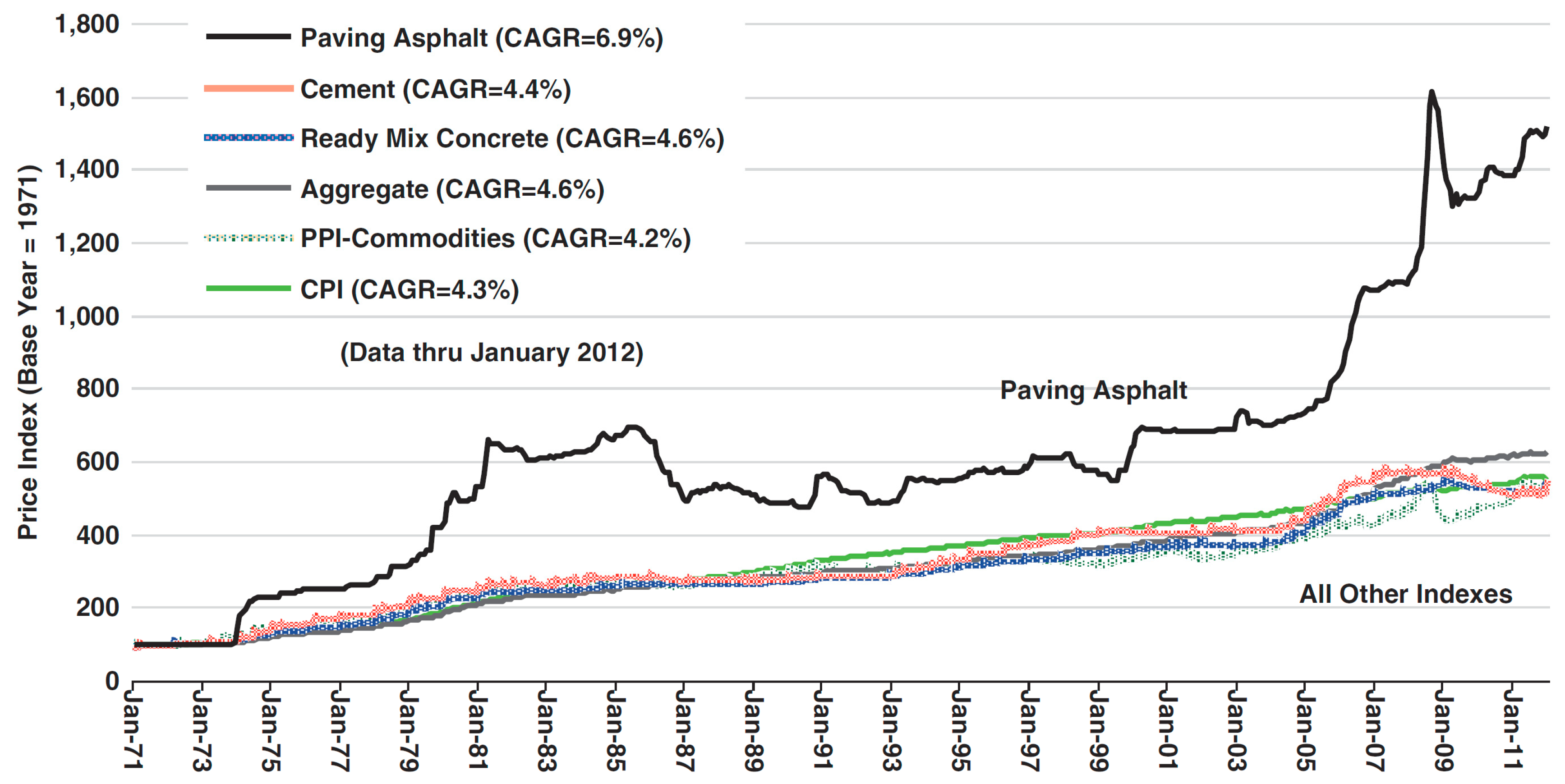
However, the construction industry grapples with the inherent volatility of material prices, as presented in Figure 1. Fluctuations in prices of essential construction materials such as steel, cement, asphalt, gravel, sand, and concrete are commonplace, driven by factors like raw material prices, energy costs, and market conditions [10,11,12]. These fluctuations pose challenges for project managers and bidders alike, making the task of material cost estimation complex and often prone to errors [13]. At the same time, the traditional econometric methods are generally reported to fail to capture the frequent changes in construction materials prices due to economic events [14,15].
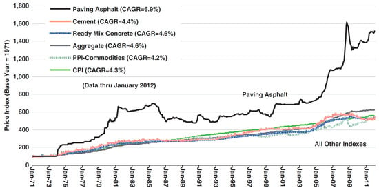
Figure 1.
Historical price trends of different common construction materials [3].
To address these challenges, data-driven techniques have emerged as a crucial tool for construction materials price forecasting [16,17,18]. These techniques leverage past data to model and predict future material prices, offering insights into potential price trends and fluctuations. They often fall under the categories of “machine learning” and “deep learning” and have been actively applied to relevant studies over the last two decades [19,20,21]. Presently, the data-driven forecasting models in the field of construction economics can broadly be classified into two categories: causal modeling and time-series analysis.
Causal models, such as multiple linear regression (MLR) and artificial neural network (ANN) models, analyze historical data alongside independent variables to forecast construction material prices [21]. Despite their widespread application in construction research, these causal models face challenges in accurately predicting future values of explanatory variables, often leading to estimation errors and high requirements on explanatory variables.
In contrast, time-series models rely solely on historical observations of construction material prices to forecast future values [22,23,24]. By identifying meaningful patterns and characteristics in the historical data, time-series models offer a cost-effective approach to price forecasting, requiring minimal data inputs for model calibration.
While numerous models exist for forecasting construction materials prices, a comprehensive synthesis and evaluation of these approaches are still lacking. Most current studies focus on developing or refining individual models, often emphasizing specific data sets or forecasting techniques. However, there is a need for a thorough review that consolidates these diverse methodologies, identifies common strengths and weaknesses, and highlights key trends and gaps in the literature. Such a synthesis would not only provide valuable insights into the most effective data-driven approaches but also guide future research efforts in addressing the persistent challenges in construction materials price forecasting.
In this paper, we delve into the importance and challenges of construction materials price forecasting, emphasizing the necessity of data-driven methodologies. We aim to summarize the characteristics of each data-driven approach, highlighting their adaptability and emphasis on leveraging large datasets to extract valuable insights. Through a comprehensive review of data-driven methodologies, we expect to contribute to the advancement of accurate and reliable construction materials price forecasting, enabling better decision-making and cost management in construction projects.
2. Research Methodology
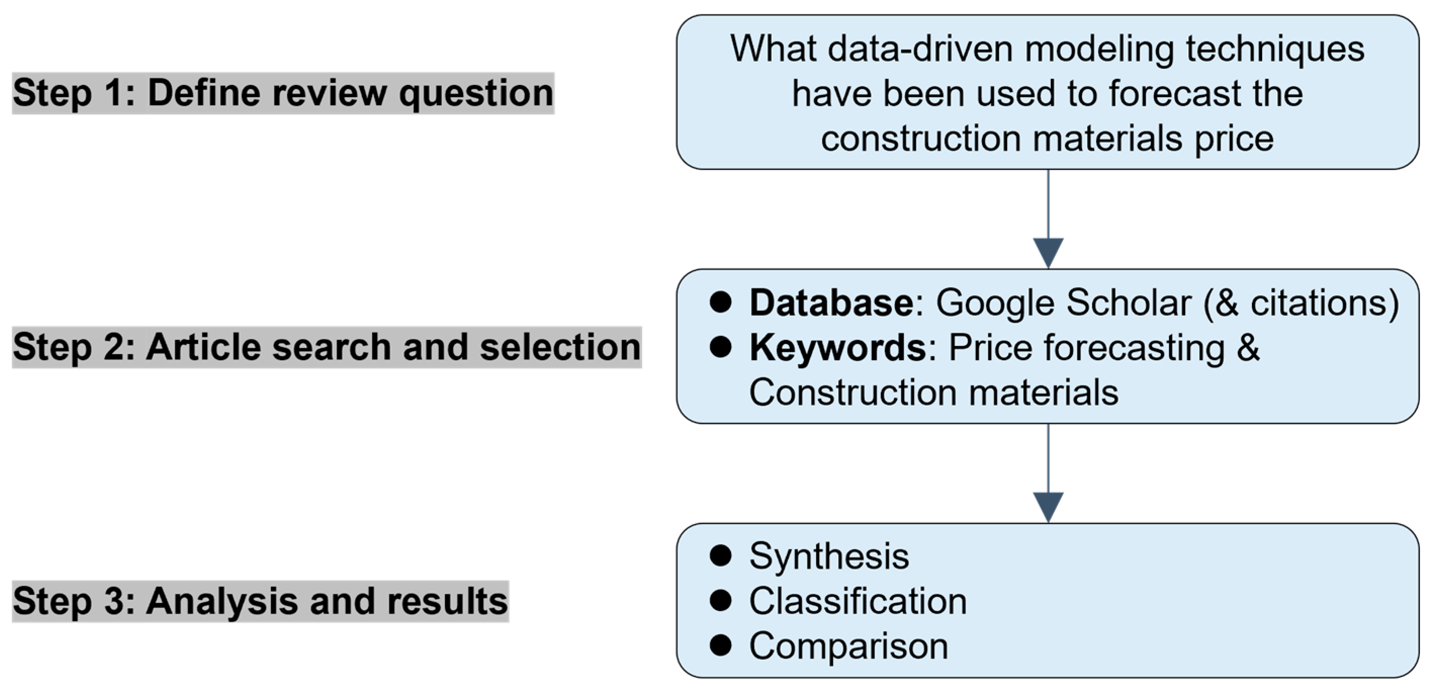
To reach a deep understanding of data-driven construction materials price forecasting, a systematic literature review methodology was applied to ensure clarity of communication, internal validity, and transparency. The methodology consists of the following three steps: (1) definition of the review question, (2) article search and selection with specific inclusion criteria, and (3) analysis and results, which were presented subsequently in Figure 2.
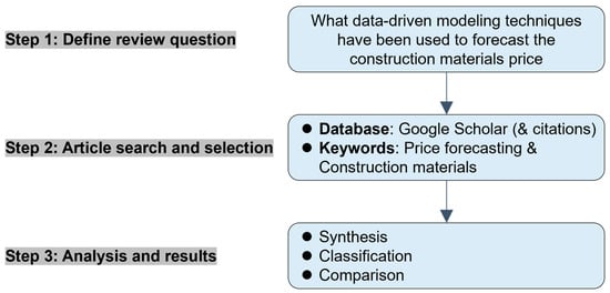
Figure 2.
Overview of research methodology.
In the first step, the review question of this study was defined as follows: What data-driven modeling techniques have been used to forecast the construction materials price?
In the second step, the relevant studies were collected from the Google Scholar database, with “price forecasting” and “construction materials” as the two keywords for the search. The rationale behind selecting these two keywords at the first step was that they were most closely related to the topic. With a comprehensive list of potentially relevant papers, further efforts were made to scan and examine each paper’s title, keywords, and abstract. If the paper was unrelated to data-driven construction materials price forecasting, it would be eliminated. After that, the references of the remaining papers were checked to include other relevant papers that were missing, and a more comprehensive list was made. Note that this step was necessary for the research methodology since it could help find the missing papers with keywords similar to the selected two, such as “price prediction” and “building materials”. Finally, a total of 60 papers on this topic were selected.
After the step of article selection, the papers were further reviewed, especially the methodology and results section, to identify the specific data-driven modeling techniques used in each paper, and the results can be seen in the following section.
3. Results and Analysis
3.1. Causal Modeling
As mentioned above, the causal models generally forecast the construction material price (as the explained variable) based on a series of explanatory variables [25]. In most cases, these explanatory variables are independent from each other. Since construction economics is, in fact, a branch of general economics, these explanatory variables are generally economic indicators, especially macroeconomic indicators [26,27,28,29].
The primary economic indicators used in the causal modeling studies related to construction economics issues, including the prediction of construction material price, construction cost index, and tender price index, are summarized in Table 1. Furthermore, the relevance of representative economic indicators—namely, the most used ones in the literature—to the construction materials price is also described in detail in Table 2.

Table 1.
Primary economic indicators identified in relevant literature to construction economics.

Table 2.
Relevance of representative economic indicators to construction materials price.
It should be noted here that in terms of predictive modeling, one of the main assumptions was that the selected input variables should be independent from each other. However, this issue was often neglected by most research works on this topic. In some studies, the explanatory variables were directly dependent. For these cases, the variables are generally selected as the historical construction material prices. In other words, historical prices, such as the prices in the last 6 months, are used as explanatory variables to predict the price in the next month. In this case, the selection of variables was questionable, and this type of model should be classified into the category of time-series analysis in essence.
The causal models used in existing relevant literature generally fall into the category of supervised machine learning, in which historical observations serve as inputs (features) alongside corresponding outcomes (labels) [43]. By analyzing these data points, the algorithm learns patterns and relationships, allowing it to make predictions on unseen data. In construction materials price forecasting, historical price data alongside relevant explanatory variables, such as economic indicators, serve as outputs and inputs to train the model.
A crucial step in causal modeling is data preparation and feature engineering. This involves preprocessing historical data to remove noise, handle missing values, and normalize features to ensure uniformity. Additionally, feature engineering entails selecting and engineering relevant features that capture underlying patterns and trends in construction materials prices. For example, feature selection is normally carried out by finding the contribution of each explanatory variable to the models’ precision and then eliminating unnecessary and repetitive variables while also maintaining the most beneficial ones. Standardization is also employed as a necessary step before feature selection since the explanatory variables generally have different magnitudes of order, and using them as-is might result in the ones with small magnitudes being overlooked.
In the process of model algorithm selection and training, supervised machine learning offers a diverse range of algorithms suited for construction materials price forecasting tasks. They range from the simplest MLR model to more complex ANN with strong nonlinear mapping ability and fault tolerance capability. The selection of an appropriate algorithm depends on the size of the price dataset and the desired interpretability of the model. Once an algorithm is chosen, the model is trained on historical price data using gradient descent or stochastic optimization to minimize prediction errors.
After training the causal model, it is essential to evaluate its performance and ensure its generalizability to unseen data. This is achieved through techniques such as cross-validation, where the dataset is divided into training and validation sets multiple times to assess the model’s performance across different data splits. Metrics such as mean absolute prediction error (MAPE), mean absolute error (MAE), mean squared error (MSE), root mean square error (RMSE), and coefficient of determination (R-squared) are commonly used to quantify the model’s accuracy and reliability in construction materials price forecasting. Once validated, the causal models can be deployed to forecast future material prices based on new data inputs.
Regarding the causal modeling of construction materials price, most existing studies proposed a single-point estimate for the price. Deterministic point predictions for the material price, however, are probably unreliable due to the various sources of uncertainty affecting the prediction results. To quantify the uncertainties, some researchers proposed to generate forecasting intervals (including the upper and lower bound of price) in a probabilistic form for construction materials price instead of a single point [44]. Therefore, in the next section, we will separately introduce both the deterministic point prediction and probabilistic interval prediction methods.
3.1.1. Point Prediction
In the algorithm list of causal models for point prediction, MLR is a linear statistical strategy for investigating the relationships between construction materials price and multiple independent explanatory variables [45].
For example, Hosny et al. employed MLR models to improve the forecasting of construction materials prices in Egypt by comparing their performance with the autoregressive integrated moving average (ARIMA) [37]. The authors collected historical price data for steel, cement, brick, ceramic, and gravel and identified 19 economic indicators that potentially influence these prices, such as GDP and unemployment rate. The research methodology involved four main processes: determining the long-term price trend and relevant indicators, validating model performance through out-of-sample projections, comparing results, and recommending the best-fitting model for each material type. The results indicated that ARIMA models were more accurate in predicting construction material prices, with a MAPE ranging from 1.4% to 2.8%. As a comparison, the range of MAPE for the MLR models was from 3% to 21%. This suggested that ARIMA was better suited for capturing the time-series nature of the price data, which was essential for accurate forecasting. The authors also acknowledged the limitations of their research, noting that the chosen indicators in MLR might not be exhaustive and that further research could explore additional indicators to improve forecasting accuracy. Similarly, Afolabi and Abimbola developed a web-based platform that used MLR algorithms to predict future prices of cement products in the Nigerian construction industry [46]. The model was trained on historical data of cement prices, petrol prices, diesel prices, interest rates, and exchange rates, achieving an 80% fit in linear regression. The rationale behind the prediction shown by the scatter plot diagram revealed that the cement increases by 250 naira biannually. Besides, when petrol prices increase by 20 naira, the interest rate increases by 1%, diesel prices increase by 50 naira, the exchange rate increases by 25 naira, and cement prices increase by 250 naira.
Owing to its capability of nonlinear fitting, the ANN algorithm has become a preferred choice of researchers for causal modeling of construction materials price [47,48,49]. The structure of a typical ANN algorithm can be seen in Figure 3.

Figure 3.
Structure of typical ANN algorithm.
Shiha et al. provided predictive tools for construction material (including steel reinforcement bars and Portland cement) prices 6 months ahead in Egypt by leveraging the ANN based on macroeconomic indicators [36,50]. The research identified leading economic indicators that influenced steel and cement prices first, including the lending rate, foreign reserves, foreign exchange rate, CPI, unemployment rate, GDP, and PPI. The models are then trained and tested using historical data from 2008 to 2018, a period marked by economic and political instabilities in Egypt. The developed ANN models showed promising results in predicting month-to-month variations in material prices while having MAPE that ranges from 4.0% to 11% for the different models. The paper also discussed the limitations of traditional econometric methods and time-series analysis in capturing sudden price changes due to economic shocks. The authors argued for the superiority of ANN models in such scenarios, highlighting their ability to learn from complex, nonlinear relationships and historical trends.
Ahmadu et al. also developed ANN models for construction material prices in Nigeria, focusing on materials susceptible to price fluctuations [30]. Utilizing a dataset from the Nigerian Bureau of Statistics (NBS), Central Bank of Nigeria (CBN), and vendors, the researchers employed a combination of ANN and Auto-encoder to create models for steel trusses, reinforcement, and Portland cement prices. The models were trained and tested using a 10-year monthly dataset, capturing significant economic changes. A total of 12 construction material price-influencing factors were considered for this study: Interest Rate, Inflation Rate, Exchange Rate, Money Supply, GDP, CPI, Lending Rate, PPI, Stock Market Indices, Monetary Policy, and Crude Oil Prices. Also, three construction materials were considered for the study, including steel trusses, reinforcement, and Portland cement. The results indicated that the Autoencoder-ANN model achieved an accuracy range of 82.04% to 96.92% and was most effective for reinforcement price prediction. Conversely, the ANN-only model, with an accuracy range of 92.87% to 98.69%, was more accurate for steel and cement prices. The study suggested that these models could support more precise estimates of construction material prices, aiding in the efficient financial management of construction projects in Nigeria. It also opened avenues for further research into the development of hybrid models that might offer improved accuracy.
Marzouk and Amin proposed the use of fuzzy logic to identify construction materials that are most sensitive to price changes at first and ANN to predict future price changes subsequently [51]. This dual approach was innovative as it combined the subjective assessment capabilities of fuzzy logic with the predictive power of neural networks. The research was based on material price changes in the Egyptian market from 2000 to 2010, which were sourced from the Central Agency for Public Mobilization and Statistics in Egypt. To be specific, this methodology involves several steps, including identifying common cost items, determining the percentage of each component in the cost item, and applying fuzzy logic to assess the importance of materials with respect to price changes. ANNs are then used to predict future prices based on historical data. To estimate the price index for a given month, two inputs are considered: (1) the price index of the last month and (2) the average general number of the last year. These inputs enable the correct representation of the characteristics of the problem, which affects the final cost of construction. The output from the NN model is the price index for the next month. The results indicated that the following materials possessed the highest impact on cost item prices: reinforced concrete (reinforcement bars), block works (blocks), insulation works (insulation materials), ceramic works (ceramic), wood works (wood), aluminum works (aluminum), tiles work (tiles), steel works (steel), and marble works (marble). Meanwhile, the training errors obtained from the neural network model ranged from 0.37 to 37.07 for the different elements, whereas the testing errors ranged from 0.04 to 36.12. The performance of ANN was compared with the MLR analysis. It was revealed that the ANN technique outperformed regression analysis with respect to the estimated error in the expected increase of the project’s elements cost. Finally, the authors demonstrated the model’s effectiveness through a numerical example of a housing project, showing how the model can predict future prices and adjust project costs accordingly.
Except for the ANN algorithm with the independent explanatory variables as inputs, several studies proposed a feed-forward time-delay neural network (TDNN) algorithm with different selection ideas of inputs. For this special type of ANN, the historical price data are used as inputs to the neural network to achieve the rolling forecasting of construction materials price. For example, use the market price of January, February, March, and April to forecast the fifth month’s market price, and use the market price of February, March, April, and May to forecast the sixth month’s market price, and so on. Finally, use the market price of June, July, August, and September to forecast the 10th month’s market price.
Ouyang et al. explored the use of TDNN for predicting steel prices, and they used the rolling forecast method to forecast the steel price, which was to use the first four months’ market price to forecast the fifth month’s price [52]. The proposed model was designed to learn from historical price data and adjust its weight values to minimize output error. The results of the study showed that the TDNN model had a strong nonlinear mapping ability and fault tolerance, making it a reliable tool for predicting material price trends.
Jha and Sinha also presented a comparative study between the TDNN and ARIMA models for forecasting agricultural commodity prices, specifically oilseeds in India [53]. The authors argued that while ARIMA models are widely used, their linearity assumption limits their ability to capture nonlinear patterns in product prices. The paper emphasized the data-driven characteristic of the TDNN model, which did not require a priori assumptions about the data’s functional relationship. Results indicated that the TDNN model outperforms the ARIMA model in terms of RMSE for nonlinear price series, suggesting its superiority for short-term price forecasting. The study also finds that the TDNN model is more effective at predicting the direction of price changes, which is valuable for understanding economic trends and making informed decisions in the market.
Kamaruddin et al. aimed to identify the most effective forecasting model for estimating the cement price index in Malaysia [54,55]. They adopted three common forecasting methods: trendlines (e.g., linear, logarithmic, polynomial), economic models (e.g., Exponential Smoothing, Holt-Winter’s Additive, and Single Moving Average), and ARIMA. At the same time, they compared those methods with TDNN using historical data. The research utilized monthly cement index data from 2005 to 2011 for Peninsular Malaysia and from 2003 to 2011 for Sabah and Sarawak. The TDNN model, with its linear transfer function, was found to produce the most accurate results based on RMSE. The paper also recommended further research into hybrid models and other neural network architectures to potentially enhance forecasting accuracy.
Except for ANN, Tang et al. introduced an advanced forecasting method for construction material prices using a combination of the least squares support vector machine (LSSVM) with an improved particle swarm optimization (IPSO) algorithm [56]. Among them, the LSSVM model was chosen for its ability to handle nonlinear regression problems, and its parameters were optimized using the IPSO algorithm to improve its performance and generalization ability [57]. The authors addressed the limitations of standard PSO, such as the tendency to fall into local optimum and premature convergence, by introducing average particle distance and fitness variance to enhance the algorithm. LSSVM was used to train the historical data of steel prices and predict the price in the next six months. The proposed IPSO-LSSVM model was tested using historical data on steel prices in Guilin, China, and the results were compared with other forecasting methods, as presented in Figure 4. The findings indicate that the IPSO-LSSVM model had superior predictive accuracy, with a MAPE of 2.11% and an MSE of 2.44%. Compared with other traditional forecasting methods such as ANN, time-series prediction, and MLR, the proposed method has the advantages of high prediction precision, fast convergence rate, and good generalization ability.
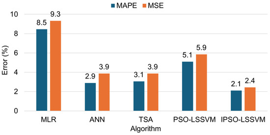
Figure 4.
Forecasting performance comparison between different algorithms [55].
3.1.2. Interval Prediction
In terms of construction materials price forecasting, the uncertainty is inescapable, but a better estimation of uncertainty results in better management and greater profitability. Therefore, some studies were motivated to predict the price interval to account for uncertainties instead of the single price point.
Mir et al. recognized that traditional machine-learning techniques often fall short due to the high uncertainties associated with material prices [44]. To overcome this, they proposed an ANN-based method to quantify uncertainties and generate forecasting intervals for construction material prices, specifically for asphalt and steel in the US market. The methodology employed the optimal lower upper bound estimation (optimal LUBE) method to train ANN for direct interval generation, as presented in Figure 5. The paper also discussed using the PPI as a proxy for material price, which was a pragmatic approach given the variability in material prices based on location.

Figure 5.
Structure of ANN algorithm for interval estimation [44].
The research methodology involves a thorough literature review to identify influential factors on material prices, data collection from reliable sources, and the application of the proposed ANN-based interval forecasting method to predict the PPI for asphalt and steel. The prediction results are compared with traditional ANN-based single-point estimates and regression analysis to validate the proposed method’s effectiveness. The findings revealed that the proposed method outperformed traditional forecasting techniques, offering more accurate prediction intervals for material prices with the narrowest prediction intervals and highest reliability. The interval forecasts provided a range within which the actual material cost is expected to fall, with a specified confidence level, as presented in Figure 6.
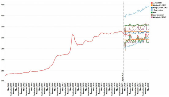
Figure 6.
Interval prediction results of optimal LUBE [44].
Overall, the ANN-based interval forecasting method demonstrated a new direction for construction materials price forecasting studies and offered a robust tool for managing price uncertainties. This approach was particularly beneficial for project managers who can make better-informed decisions about cost management and risk mitigation.
3.2. Time-Series Analysis
As another approach for construction materials price forecasting, time-series analysis focuses on studying the behavior of a variable (e.g., material prices) over discrete time intervals. It considers how a variable evolves over time, capturing trends, seasonal patterns, and irregular fluctuations. This temporal perspective allows stakeholders to uncover underlying patterns and dynamics that may influence future price movements. Time-series analysis can be classified into univariate and multivariate time-series analyses. Among them, univariate time-series analysis focuses on analyzing the behavior of a single variable, such as material prices, over time. In contrast, multivariate time-series analysis extends beyond the confines of a single variable, considering the interrelationships and dependencies among multiple variables over time. In general, the univariate time-series methods are more suitable for short-term predictions, and the multivariate time-series methods are more costly in terms of their analysis and prediction process.
3.2.1. Univariate Time-Series Analysis
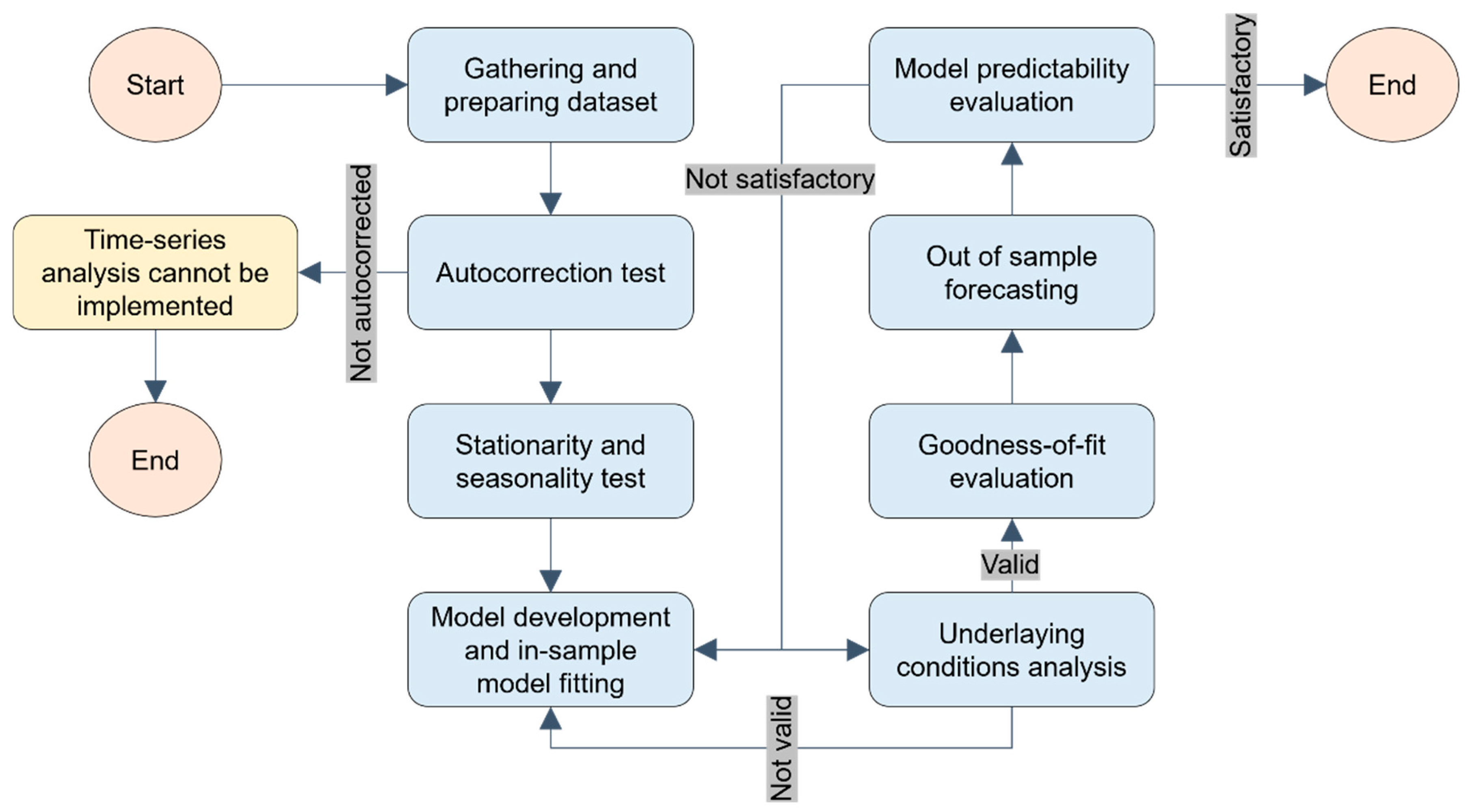
The univariate time-series analysis approach seeks to uncover patterns, trends, and seasonal fluctuations inherent in the data without considering the influence of other variables. Techniques commonly employed in univariate time-series analysis include autoregressive moving average (ARMA), ARIMA, and seasonal ARIMA. The overall workflow of univariate time-series analysis is described in Figure 7.
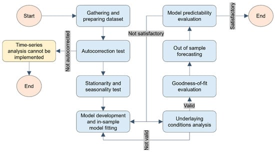
Figure 7.
Schematic diagram of univariate time-series analysis framework.
It should be noted that in conducting any econometric analysis, it is important to understand whether the data at hand exhibits stationary or nonstationary characteristics. A stationary time-series analysis is a stochastic process whose statistical properties, such as mean or variance, remain constant over time. If a time-series analysis is nonstationary (economic series are often nonstationary), however, it can frequently be transformed into a stationary process by differencing the data set (referred to as a differenced stationary process); the number of times it takes to difference the process until it becomes stationary is referred to as the order of integration. Two of the more common tests that can be used for quantifying the order of integration of a process are the augmented Dickey–Fuller (ADF) and Phillips–Perron (PP) tests.
Similar to the point prediction and interval prediction in causal modeling, the univariate time-series analysis can also be performed with or without the consideration of uncertainty. For the case without considering uncertainty, the conventional ARMA, ARIMA, and seasonal ARIMA are employed to forecast construction materials prices with some underlying assumptions (e.g., the residuals of the model follow a white-noise process and are not statistically significant). In contrast, the univariate time-series analysis considering uncertainty aims to not only forecast the price but also measure the uncertainty associated with the price fluctuations. Meanwhile, the autoregressive conditional heteroscedasticity (ARCH) and generalized autoregressive conditional heteroscedasticity (GARCH) models are employed, which are well-suited for analyzing financial time-series data that exhibit volatility clustering.
In terms of univariate time-series analysis without uncertainty consideration, for instance, Ilbeigi et al. characterized the variations in asphalt prices and developed multiple time-series forecasting models that predict future prices [58]. The authors analyzed the monthly asphalt cement price index data from Georgia over an 18-year period and identified the time-series data as autocorrelated and nonstationary, without a strong seasonal pattern. In four univariate time-series models, including Holt Exponential Smoothing (ES), Holt–Winters ES, ARIMA, and seasonal ARIMA, the ARIMA and Holt ES models prove to be the most accurate, with errors of less than 2%. Out-of-sample forecasting validates the models’ applicability, with all models demonstrating less than 4% error rates in predicting future asphalt prices.
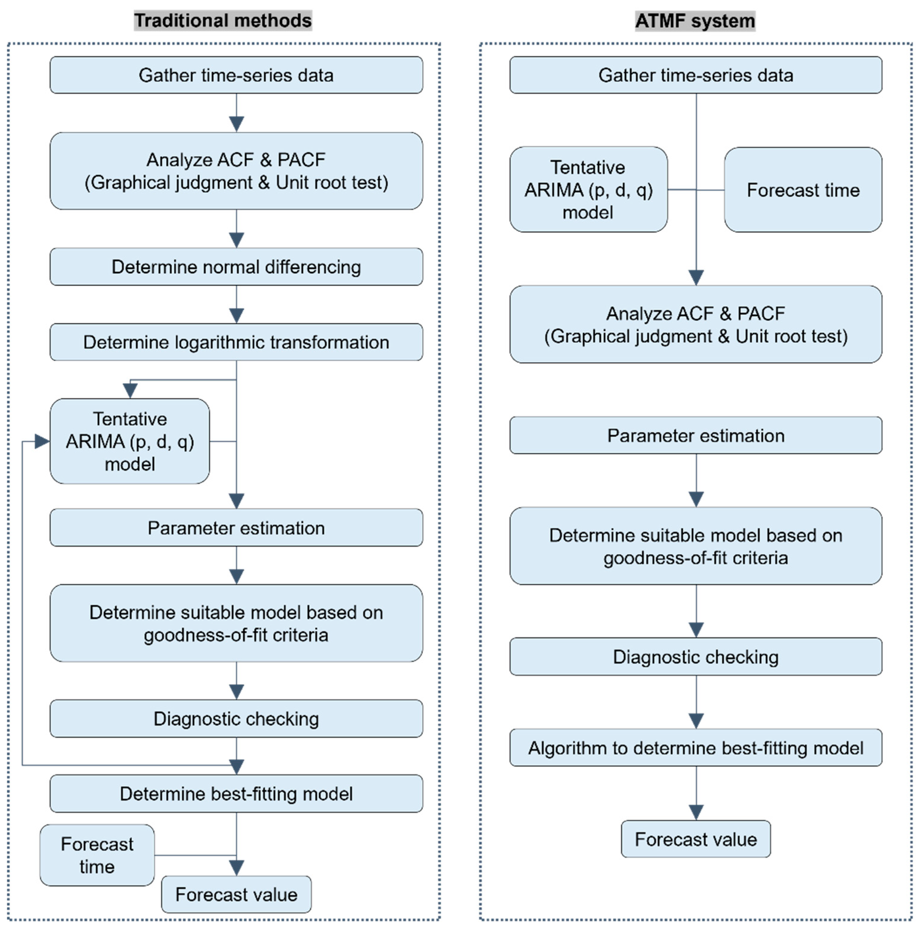
Hwang et al. also introduced an Automated Time-Series Material Cost Forecasting (ATMF) system [59]. This system is designed to address the need for a simplified and automated process for forecasting the cost escalations of numerous construction materials. The system is built on the ARIMA model and is automated to select the best-fitting forecasting model and extract forecast values, as presented in Figure 8. The research was commendable for its innovative approach to integrating auto-selected procedures and an auto-extracting module within the ATMF system. This system was evaluated using out-of-sample forecasts for three types of construction materials: high-tensile rebar, H-type steel beam, and ready-mixed concrete. The results demonstrated the system’s effectiveness, with MAPE values indicating a robust forecasting capability.
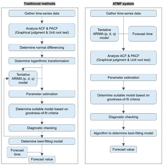
Figure 8.
Comparison between traditional time-series analysis framework and ATMF system [59].
Similarly, Yao et al., adopted an Ensemble Empirical Mode Decomposition (EEMD) method combined with the ARIMA model and Radial Basis Function (RBF) neural network to forecast cement prices [60]. This integration of EEMD was particularly noteworthy as it addressed the complexity of price fluctuations by decomposing the time-series data into intrinsic mode functions and residuals, which were then analyzed and predicted using different models. The results indicated that the EEMD-ARIMA method outperformed the EEMD-RBF method in terms of prediction accuracy, as evaluated by the RMSE, MAE, and coefficient of determination. The superior performance of the EEMD-ARIMA method could be attributed to its ability to handle the complexities of price fluctuations, including non-normality and non-linearity in the time-series data.
For the univariate time-series analysis considering uncertainty, Ilbeigi et al. further addressed the significant issue regarding the volatility and uncertainty in the asphalt price [61]. They filled a knowledge gap not only by quantifying and forecasting asphalt prices but also by measuring the uncertainty associated with price fluctuations. To be specific, the authors employed ARCH and GARCH time-series models, which are well-suited for analyzing financial time-series data that exhibit volatility clustering. The study was based on monthly asphalt price index data from the State of Georgia over an 18-year period. The research methodology involved creating a conditional mean function using an ARMA model, testing for heteroscedasticity in the residuals, and developing a GARCH model to capture the volatility of the price index. The GARCH (2,1) model, combined with an ARMA (2,2) model, is identified as the most effective for modeling the conditional volatilities in the asphalt price. The study finds that the uncertainty in the price index was significant between March 1996 and January 2002 and between July 2007 and August 2012. The model’s out-of-sample forecasting results indicated that it could predict uncertainty with less than 3% error, demonstrating its potential utility for transportation agencies in timing the implementation of risk management strategies.
In summary, to effectively measure, model, and forecast the volatility of construction material prices using univariate time-series analysis while considering uncertainty, the authors propose the following steps:
- Develop a conditional mean function.
- Conduct heteroscedasticity testing on the residuals of the mean function to assess the statistical significance of volatility.
- Employ ARCH/GARCH models if heteroscedasticity is present.
- Validate the ARCH/GARCH model by conducting heteroscedasticity testing on its residuals.
- Measure conditional volatility using the established ARCH/GARCH model.
- Evaluate the model’s performance by comparing estimated volatilities with realized volatilities.
- Perform out-of-sample forecasting for conditional volatility.
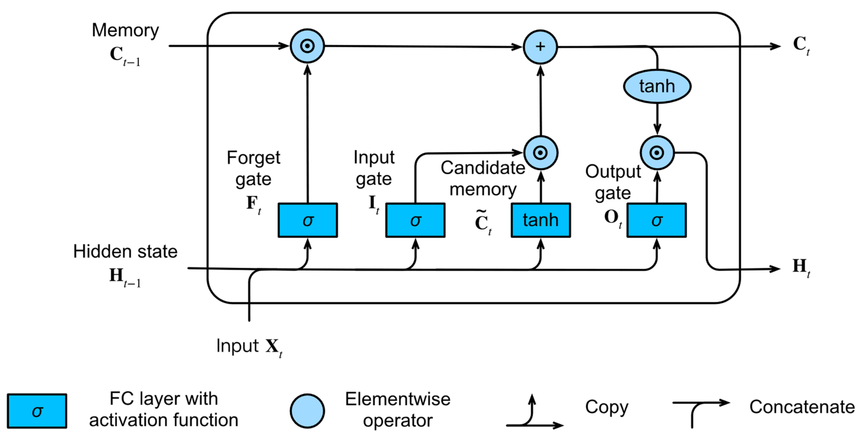
In addition to these traditional time-series models, advanced deep-learning models offer promising alternatives for construction material price forecasting [62,63,64,65]. Notably, recurrent neural networks (RNNs), specialized ANNs designed for sequential data processing, including time-series, speech, and natural language, stand out. RNNs operate as information conveyors processing data sequentially, leveraging information from previous elements to predict subsequent ones. Their recurrent layer facilitates comprehensive sequence processing, making them ideal for tasks like time-series prediction.
Moreover, within the realm of time-series networks, RNNs excel in transferring timely information through weight sharing across time steps. Specifically, the Long Short-Term Memory (LSTM) neural network overcomes RNN limitations, such as gradient vanishing and handling long-term dependencies while retaining the advantages. This advancement has been underscored in recent studies [66,67,68]. The structure of a typical LSTM neural network is presented in Figure 9.
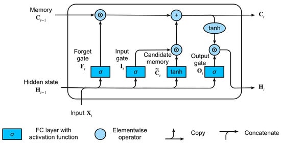
Figure 9.
Structure of typical LSTM neural network [69].
Mbah et al. applied both traditional and deep learning methods to predict limestone price variations, including the ARIMA and LSTM models [70]. The study used historical limestone price data from January 2014 to April 2020, preprocessing the data to address issues such as missing values and outliers. In particular, the LSTM model, a type of RNN capable of capturing long-term dependencies, is implemented with dropout regularization and the Adam optimizer. The performance of both models was evaluated, with the ARIMA model demonstrating higher accuracy (95.7%) compared to the LSTM model (91.8%). Additionally, the ARIMA model required less training time than the RNN model. The study suggested that the superior performance of the ARIMA model might be attributed to its auto ARIMA function, which optimized the model parameters. The issue of the advanced deep learning algorithms not achieving superior performance as expected can probably be attributed to insufficient data for modeling training or the lack of efforts in data preprocessing and feature engineering. The study also highlighted the potential for further integrating deep learning algorithms into construction materials price forecasting and suggested exploring the development of hybrid models to improve predictability.
3.2.2. Multivariate Time-Series Analysis
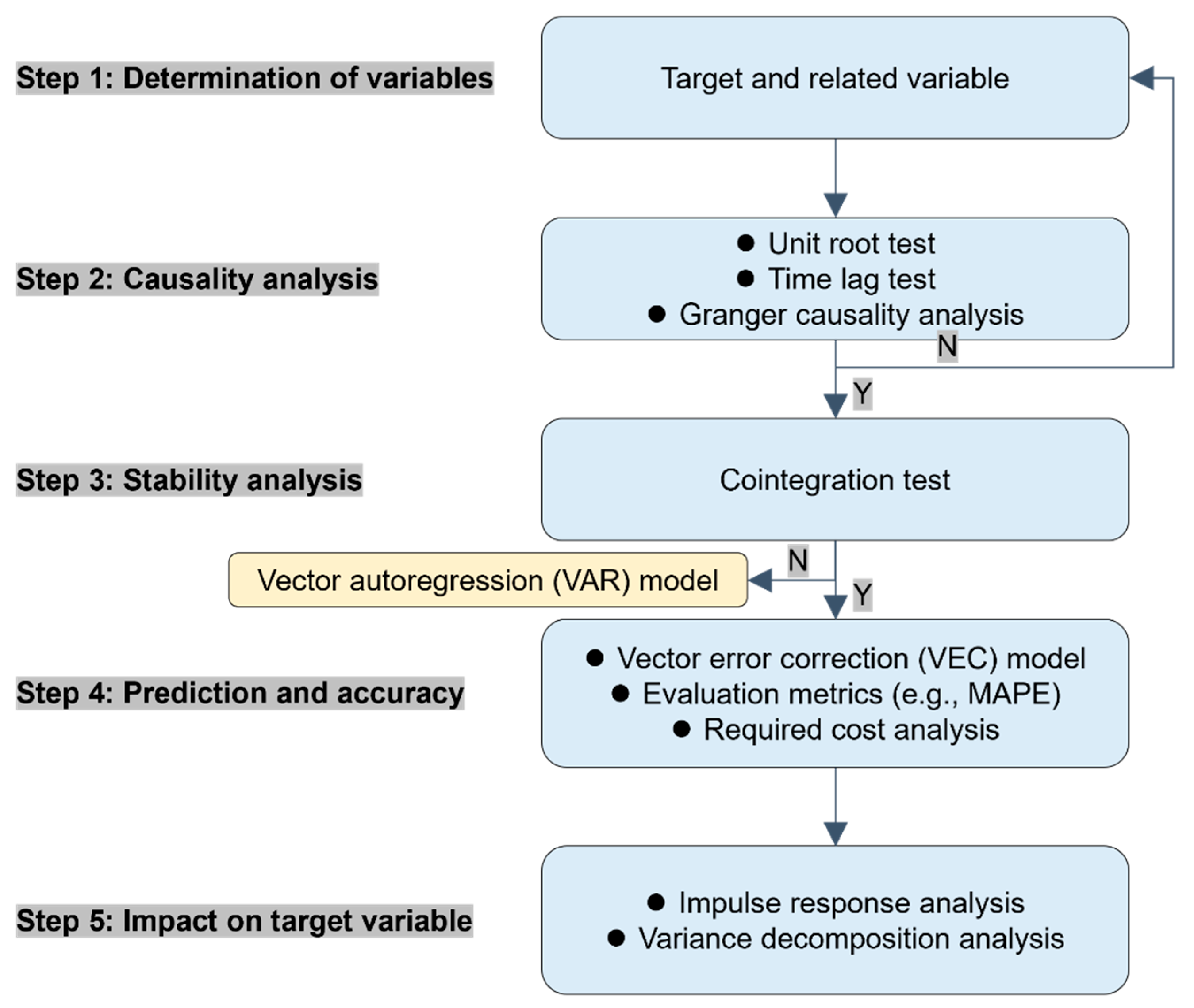
Unlike univariate, multivariate time-series analysis extends beyond the confines of a single variable, considering the interrelationships and dependencies among multiple variables over time [35]. This approach acknowledges that construction material prices may be influenced by various factors, such as market conditions, economic indicators, and industry trends. Multivariate time-series models incorporate these additional variables into the analysis, allowing stakeholders to capture more nuanced and comprehensive insights into price movements. Common techniques in multivariate analysis include vector autoregression (VAR) models, vector error correction (VEC) models, dynamic regression models, and structural time-series models [34,38,71,72]. By accounting for the interactions between different variables, multivariate time-series analysis enables stakeholders to develop more accurate and robust forecasts that are better suited to the complexities of real-world price dynamics. The typical workflow is presented in Figure 10.
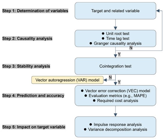
Figure 10.
Schematic diagram of multivariate time-series analysis framework [35].
Faghih and Kashani developed a VEC model for forecasting the prices of construction materials, specifically asphalt, steel, and cement, in the US [32]. A VEC model typically integrates with a VAR model, which comprehensively captures interdependencies among multiple time series with cointegration restrictions. The VAR model can be represented by the following equation:
where is vector of variables (i.e., intercept terms) at period ; is vector of constants; is coefficients matrix that describes the correlation between the considered variables; is vector of unobservable error terms; is the number of lag terms; and is the number of variables.
The preceding VAR model can then be restricted and transformed into a VEC model:
where is the identity matrix, and are the price (time series) in the period and , is the coefficient matrices of endogenous variables, and is the coefficient matrix.
When the coefficient matrix , diminishes in rank order to , it signifies the existence of cointegration relationships among the variables of interest. These relationships entail a stationary linear combination, establishing the long-run price equilibrium.
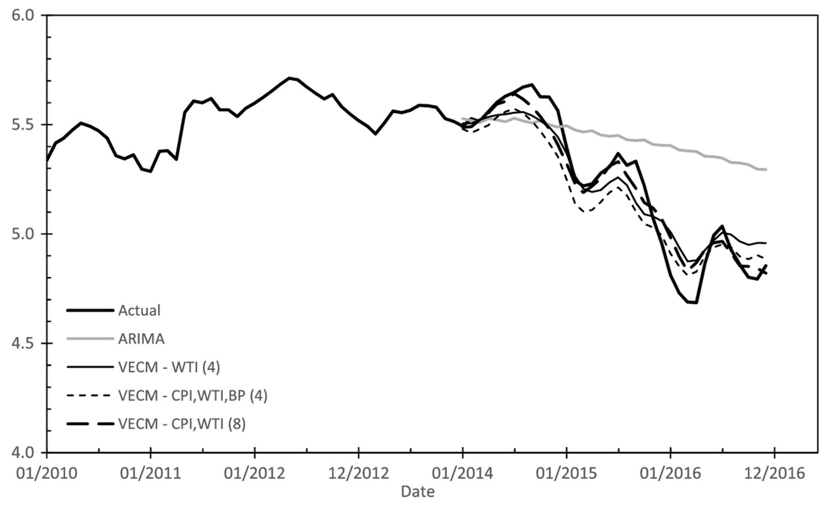
The research methodology involved the identification of candidate explanatory variables, data collection, stationarity testing, causality testing, cointegration testing, and the construction of VEC models. The explanatory variables included in this study were CPI, West Texas Intermediate (WTI), building permits (BP), crude oil price, and so on. One of the strengths of this study is its use of the Johansen cointegration test to establish long-term relationships between variables, which is a crucial step in the development of VEC models. The VEC model’s performance was further compared with that of univariate time-series models, such as ARIMA, demonstrating the superior predictive capabilities of the VEC model, as presented in Table 3 and Figure 11. Overall, the authors addressed a critical gap by addressing the need for models that could predict both short- and long-term price movements of individual construction materials, which was essential for accurate cost estimation and project planning.

Table 3.
Forecasting performance comparison of different time-series models.
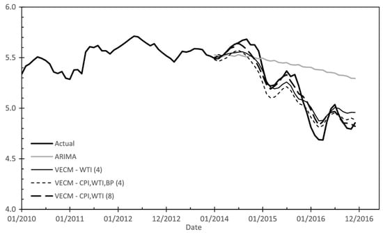
Figure 11.
Comparison of actual asphalt prices with those forecasts using ARIMA and VEC models [32].
Swei et al. also introduced a probabilistic hybrid forecasting model for long-term price projections of construction materials, specifically concrete and asphalt [73,74]. The model was designed to provide expected price projections and quantify the uncertainty associated with future price movements. The authors implement a four-step methodology that includes establishing a long-run price trend between paving materials and their constituents with VEC models, projecting future prices of relevant constituents and paving materials using Monte Carlo simulations, and validating the model’s performance through out-of-sample forecasts. Specifically, the probabilistic price forecasting equations of asphalt and concrete were derived by the integration of constituent models within the long-term price equilibrium. Finally, they found that the proposed model performed similarly to current practice regarding expected price projections but offered a significant advantage in providing theoretical uncertainty bounds that closely matched future volatility. This was crucial for decision-makers who must account for risk in their investment choices.
3.3. Monte Carlo Simulation
Besides the commonly utilized causal modeling and time-series analysis, the Monte Carlo simulation is another noteworthy statistical method for forecasting construction materials prices. Widely employed in predicting construction project costs, this approach stands out for its ability to model short-term variations in construction materials prices [75]. While methods like applying a fixed percentage of the total cost as a risk premium or inflating estimated material costs to the expected midpoint of the construction date exist, only the Monte Carlo approach can effectively capture these short-term fluctuations. However, its predictability hinges greatly on the accuracy of input distributions and lacks consideration for autocorrelation in historical price trends and causal inference with other indicators. Essentially, it generates random values for material price escalation rates based on histograms, making it more suitable for assessing price ranges.
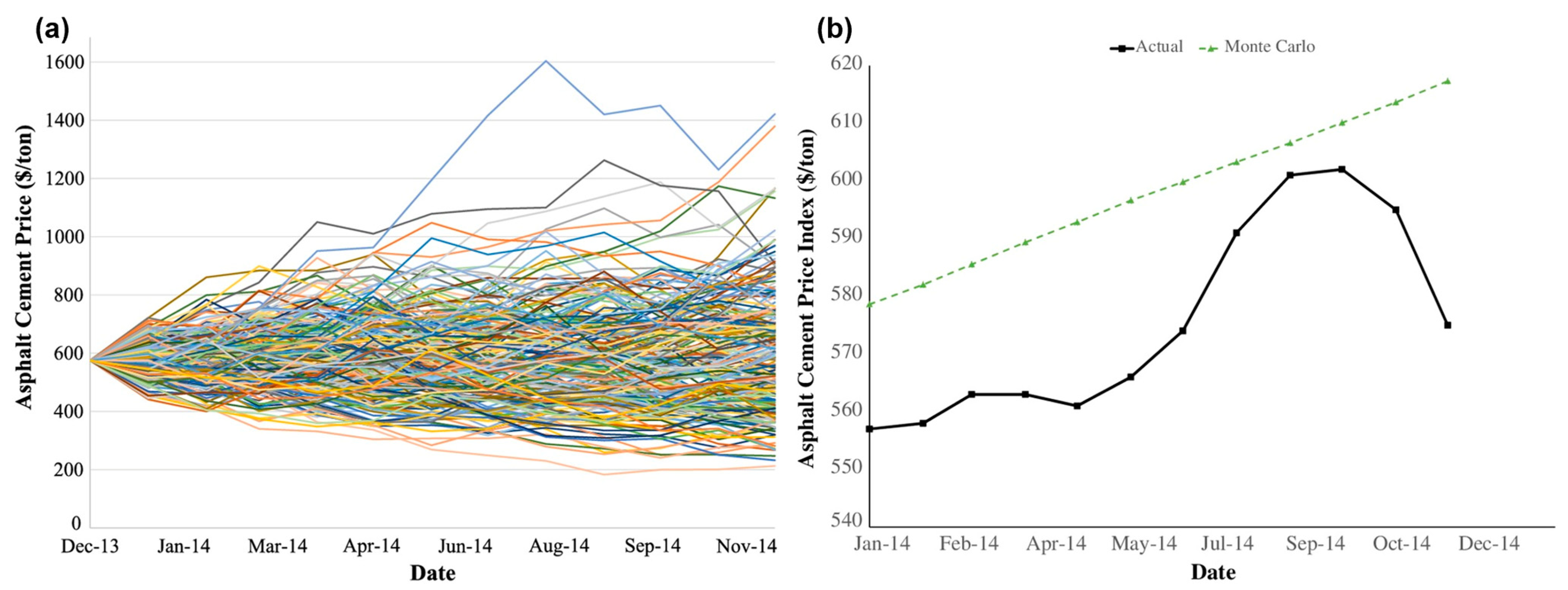
In a study by Ilbeigi et al., a Monte Carlo simulation model was developed to forecast future asphalt prices and compared against other time-series forecasting models like ARIMA [58]. Initially, the histogram of historical asphalt price escalation rates was fitted with a triangular distribution [76]. Subsequently, over 100,000 random paths were generated during the simulation process. At each time point in the out-of-sample period, the average value of simulated future asphalt cement prices was calculated. Figure 12 illustrates the expected values of future asphalt cement prices calculated by the Monte Carlo simulation and compares them to actual values. Notably, the Monte Carlo simulation’s three error measures, including MAPE, MSE, and MAE, were higher than those of other time-series models. The authors reasoned that this discrepancy stemmed from Monte Carlo simulations inadequately addressing the autocorrelation present in historical price data.

Figure 12.
Monte Carlo simulation, (a) Random simulation results of future asphalt price; (b) Average value of simulated future asphalt price [58].
4. Summary and Discussion
In summary, the advantages and disadvantages of each data-driven modeling technique mentioned in the above section and the corresponding references are discussed, as presented in Table 4.

Table 4.
Summary of data-driven construction materials price forecasting methods.
5. Conclusions
In conclusion, the accurate forecasting of construction material prices is paramount for the financial management and overall success of construction projects. This review has comprehensively examined the various data-driven methodologies for predicting price trends and fluctuations in the construction industry. Furthermore, accurate price predictions enable construction firms to manage costs better, reduce financial risks, and improve project planning and budgeting. This, in turn, contributes to more stable construction markets, which is beneficial for economic growth and infrastructure development.
Causal modeling, particularly through MLR and ANN, has been widely applied but faces challenges in capturing the nonlinear and complex relationships inherent in price volatility. Time-series analysis, both univariate and multivariate, offers a more focused approach by analyzing historical price data for pattern recognition, which is crucial for short-term predictions. Integrating advanced algorithms, such as LSSVM and LSTM, has demonstrated improved predictive accuracy and generalization capabilities. Furthermore, the use of Monte Carlo simulation also provides a probabilistic approach to account for uncertainties in price forecasting, although it is limited by its reliance on accurate input distributions. Overall, the causal modeling methodology is a preferred choice of practitioners if sufficient information and data (e.g., macroeconomic indicators) related to the material price are available for the modeling, in particular with the assistance of machine learning techniques. On the other hand, if only historical materials price data can be accessed, it is more recommended to adopt the time-series analysis methodology, mining the inherent trends in historical data for future price forecasting.
For future studies, the review highlights that hybrid models, which combine the strengths of different forecasting techniques, may present the most effective solution for construction material price prediction. These models leverage the predictive power of machine learning while incorporating the temporal analysis strengths of time-series methods. Meanwhile, developing deep learning-advanced time-series analysis models, supported by rigorous data preparation and feature engineering, also offers a promising direction for future relevant research. As the construction industry continues to evolve, the adoption of these advanced forecasting methods will be instrumental in navigating market uncertainties and optimizing project cost estimation and management.
Author Contributions
Conceptualization: J.M. and T.W.; Methodology: Q.L.; Investigation: P.H. and S.P.; Resources: J.M. and T.W.; Data curation: Q.L.; Writing—original draft: Q.L. and J.M.; Writing—review and editing: J.M. and T.W.; Visualization: Q.L.; Supervision: J.M.; Project administration: T.W.; Funding acquisition: J.M. and T.W. All authors have read and agreed to the published version of the manuscript.
Funding
This study is supported by Fundamental Research Funds for the Central Universities (Nos. 2023JBMC049) and the National Natural Science Foundation of China (Grant Nos. 52108392).
Conflicts of Interest
Author Peikai He and Si Peng are employed by the Taihang Urban and Rural Construction Group Co., Ltd. The remaining authors declare that the research was conducted in the absence of any commercial or financial relationships that could be construed as a potential conflict of interest.
References
- Mirzadeh, I.; Birgisson, B. Accommodating Energy Price Volatility in Life Cycle Cost Analysis of Asphalt Pavements. J. Civ. Eng. Manag. 2015, 22, 1001–1008. [Google Scholar] [CrossRef][Green Version]
- Abdul Nabi, M.; Chammout, B.; El-adaway, I.H.; Assaad, R.H.; Assaf, G. Investigating Price Fluctuation Transmission among Construction Materials. In Proceedings of the Construction Research Congress, Des Moines, IA, USA, 20–23 March 2024; American Society of Civil Engineers: Des Moines, IA, USA, 2024; pp. 339–349. [Google Scholar]
- Mack, J.W. Accounting for Material-Specific Inflation Rates in Life-Cycle Cost Analysis for Pavement Type Selection. Transp. Res. Rec. 2012, 2304, 86–96. [Google Scholar] [CrossRef]
- Musarat, M.A.; Alaloul, W.S.; Liew, M.S.; Maqsoom, A.; Qureshi, A.H. Investigating the Impact of Inflation on Building Materials Prices in Construction Industry. J. Build. Eng. 2020, 32, 101485. [Google Scholar] [CrossRef]
- Bilec, M.M.; Marriott, J.; Padilla, M.F.; Snyder, M. Market Analysis of Construction Materials with Recommendations for the Future of the Industry; University of Pittsburgh: Pittsburgh, PA, USA, 2010. [Google Scholar]
- Lee, C.; Lee, E.-B. Prediction Method of Real Discount Rate to Improve Accuracy of Life-Cycle Cost Analysis. Energy Build. 2017, 135, 225–232. [Google Scholar] [CrossRef]
- Cardinal, K.M.; Khalafalla, M.; Rueda-Benavides, J.A. Development of a Stochastic Risk Assessment Protocol for Analyzing the Impact of Fluctuations in Crude Oil and Fuel Prices on Asphalt Prices in the State of Alabama. In Proceedings of the Construction Research Congress, Des Moines, IA, USA, 20–23 March 2024; American Society of Civil Engineers: Des Moines, IA, USA, 2024; pp. 196–206. [Google Scholar]
- Cardinal, K.M.; Khalafalla, M.; Rueda-Benavides, J. Protocol to Assess the Impact of Crude Oil Price Fluctuations on Future Asphalt Prices. Transp. Res. Rec. 2021, 2675, 294–305. [Google Scholar] [CrossRef]
- Akanni, P.O.; Oke, A.E.; Omotilewa, O.J. Implications of Rising Cost of Building Materials in Lagos State Nigeria. SAGE Open 2014, 4, 215824401456121. [Google Scholar] [CrossRef]
- Elfahham, Y. Estimation and Prediction of Construction Cost Index Using Neural Networks, Time Series, and Regression. Alex. Eng. J. 2019, 58, 499–506. [Google Scholar] [CrossRef]
- Ng, S.T.; Cheung, S.O.; Martin Skitmore, R.; Lam, K.C.; Wong, L.Y. Prediction of Tender Price Index Directional Changes. Constr. Manag. Econ. 2000, 18, 843–852. [Google Scholar] [CrossRef]
- Olatunji, O.A. The Impact of Oil Price Regimes on Construction Cost in Nigeria. Constr. Manag. Econ. 2010, 28, 747–759. [Google Scholar] [CrossRef]
- Meglin, R.; Kytzia, S.; Habert, G. Uncertainty, Variability, Price Changes and Their Implications on a Regional Building Materials Industry: The Case of Swiss Canton Argovia. J. Clean. Prod. 2022, 330, 129944. [Google Scholar] [CrossRef]
- Chaitongrat, T.; Janthachai, K.; Kusonkhum, W.; Boonchai, P.; Ikhwali, M.F.; Khotdee, M. Comparing Data Mining Methods for Predicting Cost Construction Projects: A Case Study of Cost Management Datasets from Thailand. J. Infras. Policy Dev. 2024, 8, 2801. [Google Scholar] [CrossRef]
- Mahdavian, A.; Shojaei, A.; Salem, M.; Yuan, J.S.; Oloufa, A.A. Data-Driven Predictive Modeling of Highway Construction Cost Items. J. Constr. Eng. Manag. 2021, 147, 04020180. [Google Scholar] [CrossRef]
- Kim, C.; Khan, G.; Nguyen, B.; Hoang, E.L. Development of a Statistical Model to Predict Materials’ Unit Prices for Future Maintenance and Rehabilitation in Highway Life Cycle Cost Analysis; Mineta Transportation Institute: San Jose, CA, USA, 2020. [Google Scholar]
- Lee, C.-Y.; Chou, B.-J.; Huang, C.-F. Data Science and Reinforcement Learning for Price Forecasting and Raw Material Procurement in Petrochemical Industry. Adv. Eng. Inform. 2022, 51, 101443. [Google Scholar] [CrossRef]
- Wang, Q.K.; Mei, T.T.; Guo, Z.; Kong, L.W. Building Material Price Forecasting Based on Multi-Method in China. In Proceedings of the 2018 IEEE International Conference on Industrial Engineering and Engineering Management (IEEM), Bangkok, Thailand, 16–19 December 2018; IEEE: Bangkok, Thailand, 2018; pp. 1826–1830. [Google Scholar]
- Bassioni, H.A.; Elmasry, M.I.; Ragheb, A.M. Time Series Analysis for the Prediction of RC Material Components Prices in Egypt. In Proceedings of the 28th Annual ARCOM Conference, Edinburgh, UK, 3–5 September 2012; Association of Researchers in Construction Management: Edinburgh, UK, 2012; pp. 381–390. [Google Scholar]
- Deb, C.; Zhang, F.; Yang, J.; Lee, S.E.; Shah, K.W. A Review on Time Series Forecasting Techniques for Building Energy Consumption. Renew. Sustain. Energy Rev. 2017, 74, 902–924. [Google Scholar] [CrossRef]
- Hwang, S. Dynamic Regression Models for Prediction of Construction Costs. J. Constr. Eng. Manag. 2009, 135, 360–367. [Google Scholar] [CrossRef]
- Ashuri, B.; Lu, J. Time Series Analysis of ENR Construction Cost Index. J. Constr. Eng. Manag. 2010, 136, 1227–1237. [Google Scholar] [CrossRef]
- Hwang, S. Time Series Models for Forecasting Construction Costs Using Time Series Indexes. J. Constr. Eng. Manag. 2011, 137, 656–662. [Google Scholar] [CrossRef]
- Joukar, A.; Nahmens, I. Volatility Forecast of Construction Cost Index Using General Autoregressive Conditional Heteroskedastic Method. J. Constr. Eng. Manag. 2016, 142, 04015051. [Google Scholar] [CrossRef]
- Cao, Y.; Ashuri, B.; Baek, M. Prediction of Unit Price Bids of Resurfacing Highway Projects through Ensemble Machine Learning. J. Comput. Civ. Eng. 2018, 32, 04018043. [Google Scholar] [CrossRef]
- Akintoye, A.; Bowen, P.; Hardcastle, C. Macro-Economic Leading Indicators of Construction Contract Prices. Constr. Manag. Econ. 1998, 16, 159–175. [Google Scholar] [CrossRef]
- Ashuri, B.; Shahandashti, S.M.; Lu, J. Empirical Tests for Identifying Leading Indicators of ENR Construction Cost Index. Constr. Manag. Econ. 2012, 30, 917–927. [Google Scholar] [CrossRef]
- Chen, H.L. Using Financial and Macroeconomic Indicators to Forecast Sales of Large Development and Construction Firms. J. Real Estate Finan. Econ. 2010, 40, 310–331. [Google Scholar] [CrossRef]
- Ernest, K.; Theophilus, A.-K.; Amoah, P.; Emmanuel, B.B. Identifying Key Economic Indicators Influencing Tender Price Index Prediction in the Building Industry: A Case Study of Ghana. Int. J. Constr. Manag. 2019, 19, 106–112. [Google Scholar] [CrossRef]
- Ahmadu, H.A.; Ibrahim, Y.M.; Abdulrahman, R.S.; Jibril, U.S.; Yamusa, M.A. Developing Machine Learning Prediction Models for Construction Material Prices in Nigeria. ATBU J. Environ. Technol. 2023, 16, 22–42. [Google Scholar]
- Cao, M.-T.; Cheng, M.-Y.; Wu, Y.-W. Hybrid Computational Model for Forecasting Taiwan Construction Cost Index. J. Constr. Eng. Manag. 2015, 141, 04014089. [Google Scholar] [CrossRef]
- Faghih, S.A.M.; Kashani, H. Forecasting Construction Material Prices Using Vector Error Correction Model. J. Constr. Eng. Manag. 2018, 144, 04018075. [Google Scholar] [CrossRef]
- Ng, S.T.; Cheung, S.O.; Skitmore, M.; Wong, T.C.Y. An Integrated Regression Analysis and Time Series Model for Construction Tender Price Index Forecasting. Constr. Manag. Econ. 2004, 22, 483–493. [Google Scholar] [CrossRef]
- Shahandashti, S.M.; Ashuri, B. Highway Construction Cost Forecasting Using Vector Error Correction Models. J. Manag. Eng. 2016, 32, 04015040. [Google Scholar] [CrossRef]
- Shahandashti, S.M.; Ashuri, B. Forecasting Engineering News-Record Construction Cost Index Using Multivariate Time Series Models. J. Constr. Eng. Manag. 2013, 139, 1237–1243. [Google Scholar] [CrossRef]
- Shiha, A.; Dorra, E.M.; Nassar, K. Neural Networks Model for Prediction of Construction Material Prices in Egypt Using Macroeconomic Indicators. J. Constr. Eng. Manag. 2020, 146, 04020010. [Google Scholar] [CrossRef]
- Hosny, S.; Elsaid, E.; Hosny, H. Prediction of Construction Material Prices Using ARIMA and Multiple Regression Models. Asian J. Civ. Eng. 2023, 24, 1697–1710. [Google Scholar] [CrossRef]
- Jiang, H.; Xu, Y.; Liu, C. Construction Price Prediction Using Vector Error Correction Models. J. Constr. Eng. Manag. 2013, 139, 04013022. [Google Scholar] [CrossRef]
- Zhou, H.; Zhao, J.H. Analysis on Factors to Cause the Price Change of Building Materials. Adv. Mater. Res. 2013, 683, 668–671. [Google Scholar] [CrossRef]
- Ramadan, M. Development and Prediction of a Construction Price Index in Egypt. Master’s Thesis, American University in Cairo, New Cairo, Egypt, 2023. [Google Scholar]
- Wong, J.M.W.; Ng, S.T. Forecasting Construction Tender Price Index in Hong Kong Using Vector Error Correction Model. Constr. Manag. Econ. 2010, 28, 1255–1268. [Google Scholar] [CrossRef]
- Oladipo, F.; Oni, O. Review of Selected Macroeconomic Factors Impacting Building Material Prices in Developing Countries—A Case of Nigeria. Ethiop. J. Environ. Stud. Manag. 2012, 5, 131–137. [Google Scholar] [CrossRef]
- Chakraborty, D.; Elhegazy, H.; Elzarka, H.; Gutierrez, L. A Novel Construction Cost Prediction Model Using Hybrid Natural and Light Gradient Boosting. Adv. Eng. Inform. 2020, 46, 101201. [Google Scholar] [CrossRef]
- Mir, M.; Kabir, H.M.D.; Nasirzadeh, F.; Khosravi, A. Neural Network-Based Interval Forecasting of Construction Material Prices. J. Build. Eng. 2021, 39, 102288. [Google Scholar] [CrossRef]
- Lowe, D.J.; Emsley, M.W.; Harding, A. Predicting Construction Cost Using Multiple Regression Techniques. J. Constr. Eng. Manag. 2006, 132, 750–758. [Google Scholar] [CrossRef]
- Afolabi, A.O.; Abimbola, O. Application of Machine Learning in Cement Price Prediction through a Web-Based System. IJECE 2022, 12, 5214. [Google Scholar] [CrossRef]
- Issa, R.R.A. Application of Artificial Neural Networks to Predicting Construction Material Prices. In Proceedings of the Computing in Civil and Building Engineering (2000), Stanford, CA, USA, 4 August 2000; American Society of Civil Engineers: Stanford, CA, USA, 2000; pp. 1129–1132. [Google Scholar]
- Williams, T.P. Predicting Changes in Construction Cost Indexes Using Neural Networks. J. Constr. Eng. Manag. 1994, 120, 306–320. [Google Scholar] [CrossRef]
- Wilmot, C.G.; Mei, B. Neural Network Modeling of Highway Construction Costs. J. Constr. Eng. Manag. 2005, 131, 765–771. [Google Scholar] [CrossRef]
- Shiha, A. Prediction of Construction Material Prices Using Macroeconomic Indicators: A Neural Networks Model; American University in Cairo: New Cairo, Egypt, 2019. [Google Scholar]
- Marzouk, M.; Amin, A. Predicting Construction Materials Prices Using Fuzzy Logic and Neural Networks. J. Constr. Eng. Manag. 2013, 139, 1190–1198. [Google Scholar] [CrossRef]
- Ouyang, H.; Zhang, X.; Hu, C. Application Research on the Artificial Neural Network in the Building Materials Price Prediction. In the 19th International Conference on Industrial Engineering and Engineering Management; Qi, E., Shen, J., Dou, R., Eds.; Springer: Berlin/Heidelberg, Germany, 2013; pp. 167–175. ISBN 978-3-642-38432-5. [Google Scholar]
- Jha, G.K.; Sinha, K. Time-Delay Neural Networks for Time Series Prediction: An Application to the Monthly Wholesale Price of Oilseeds in India. Neural Comput. Applic. 2014, 24, 563–571. [Google Scholar] [CrossRef]
- Kamaruddin, S.B.A.; Ghani, N.A.M.; Ramli, N.M. Determining the Best Forecasting Model of Cement Price Index in Malaysia. In Proceedings of the 2012 IEEE Colloquium on Humanities, Science and Engineering (CHUSER), Kota Kinabalu, Malaysia, 3–4 December 2012; IEEE: Kota Kinabalu, Malaysia, 2012; pp. 524–528. [Google Scholar]
- Kamaruddin, S.B.A.; Ghani, N.A.M.; Ramli, N.M. Estimating Cement Price Index by Regions in Peninsular Malaysia. In Proceedings of the 2012 International Conference on Statistics in Science, Business and Engineering (ICSSBE), Langkawi, Malaysia, 10–12 September 2012; IEEE: Langkawi, Malaysia, 2012; pp. 1–4. [Google Scholar]
- Tang, B.; Han, J.; Guo, G.; Chen, Y.; Zhang, S. Building Material Prices Forecasting Based on Least Square Support Vector Machine and Improved Particle Swarm Optimization. Archit. Eng. Des. Manag. 2019, 15, 196–212. [Google Scholar] [CrossRef]
- Zhang, J.-L.; Zhang, Y.-J.; Zhang, L. A Novel Hybrid Method for Crude Oil Price Forecasting. Energy Econ. 2015, 49, 649–659. [Google Scholar] [CrossRef]
- Ilbeigi, M.; Ashuri, B.; Joukar, A. Time-Series Analysis for Forecasting Asphalt-Cement Price. J. Manag. Eng. 2017, 33, 04016030. [Google Scholar] [CrossRef]
- Hwang, S.; Park, M.; Lee, H.-S.; Kim, H. Automated Time-Series Cost Forecasting System for Construction Materials. J. Constr. Eng. Manag. 2012, 138, 1259–1269. [Google Scholar] [CrossRef]
- Yao, F.; Zeng, H.; Liu, T.; Wu, Y. Research on Cement Price Fluctuation Prediction Based on EEMD-ARIMA. In Proceedings of the 27th International Symposium on Advancement of Construction Management and Real Estate; Li, J., Lu, W., Peng, Y., Yuan, H., Wang, D., Eds.; Lecture Notes in Operations Research; Springer Nature Singapore: Singapore, 2023; pp. 324–339. ISBN 978-981-9936-25-0. [Google Scholar]
- Ilbeigi, M.; Castro-Lacouture, D.; Joukar, A. Generalized Autoregressive Conditional Heteroscedasticity Model to Quantify and Forecast Uncertainty in the Price of Asphalt Cement. J. Manag. Eng. 2017, 33, 04017026. [Google Scholar] [CrossRef]
- Li, B.; Xin, Q.; Zhang, L. Engineering Cost Prediction Model Based on DNN. Sci. Program. 2022, 2022, 3257856. [Google Scholar] [CrossRef]
- Mao, S.; Tseng, C.-H.; Shang, J.; Wu, Y.; Zeng, X.-J. Construction Cost Index Prediction: A Visibility Graph Network Method. In Proceedings of the 2021 International Joint Conference on Neural Networks (IJCNN), Shenzhen, China, 18 July 2021; IEEE: Shenzhen, China, 2021; pp. 1–6. [Google Scholar]
- Nelson, M.; Hill, T.; Remus, W.; O’Connor, M. Time Series Forecasting Using Neural Networks: Should the Data Be Deseasonalized First? J. Forecast. 1999, 18, 359–367. [Google Scholar] [CrossRef]
- Sezer, O.B.; Gudelek, M.U.; Ozbayoglu, A.M. Financial Time Series Forecasting with Deep Learning: A Systematic Literature Review: 2005–2019. Appl. Soft Comput. 2020, 90, 106181. [Google Scholar] [CrossRef]
- Dong, J.; Chen, Y.; Guan, G. Cost Index Predictions for Construction Engineering Based on LSTM Neural Networks. Adv. Civ. Eng. 2020, 2020, 6518147. [Google Scholar] [CrossRef]
- Kumar Dubey, A.; Kumar, A.; García-Díaz, V.; Kumar Sharma, A.; Kanhaiya, K. Study and Analysis of SARIMA and LSTM in Forecasting Time Series Data. Sustain. Energy Technol. Assess. 2021, 47, 101474. [Google Scholar] [CrossRef]
- Wang, C.; Qiao, J. Construction Project Cost Prediction Method Based on Improved BiLSTM. Appl. Sci. 2024, 14, 978. [Google Scholar] [CrossRef]
- Cao, Y.; Ashuri, B. Predicting the Volatility of Highway Construction Cost Index Using Long Short-Term Memory. J. Manag. Eng. 2020, 36, 04020020. [Google Scholar] [CrossRef]
- Mbah, T.J.; Ye, H.; Zhang, J.; Long, M. Using LSTM and ARIMA to Simulate and Predict Limestone Price Variations. Min. Metall. Explor. 2021, 38, 913–926. [Google Scholar] [CrossRef]
- Lee, C.; Won, J.; Lee, E.-B. Method for Predicting Raw Material Prices for Product Production over Long Periods. J. Constr. Eng. Manag. 2019, 145, 05018017. [Google Scholar] [CrossRef]
- Xu, J.; Moon, S. Stochastic Forecast of Construction Cost Index Using a Cointegrated Vector Autoregression Model. J. Manag. Eng. 2013, 29, 10–18. [Google Scholar] [CrossRef]
- Swei, O.; Gregory, J.; Kirchain, R. Probabilistic Approach for Long-Run Price Projections: Case Study of Concrete and Asphalt. J. Constr. Eng. Manag. 2017, 143, 05016018. [Google Scholar] [CrossRef]
- Swei, O.A. Incorporating Uncertainty in the Life Cycle Cost Analysis of Pavements; Massachusetts Institute of Technology: Cambridge, MA, USA, 2012. [Google Scholar]
- Wang, Y.; Liu, M. Prices of Highway Resurfacing Projects in Economic Downturn: Lessons Learned and Strategies Forward. J. Manag. Eng. 2012, 28, 391–397. [Google Scholar] [CrossRef]
- Back, W.E.; Boles, W.W.; Fry, G.T. Defining Triangular Probability Distributions from Historical Cost Data. J. Constr. Eng. Manag. 2000, 126, 29–37. [Google Scholar] [CrossRef]
- Oshodi, O.; Ejohwomu, O.A.; Famakin, I.O.; Cortez, P. Comparing Univariate Techniques for Tender Price Index Forecasting: Box-Jenkins and Neural Network Model. CEB 2017, 17, 109–123. [Google Scholar] [CrossRef]
Disclaimer/Publisher’s Note: The statements, opinions and data contained in all publications are solely those of the individual author(s) and contributor(s) and not of MDPI and/or the editor(s). MDPI and/or the editor(s) disclaim responsibility for any injury to people or property resulting from any ideas, methods, instructions or products referred to in the content. |
© 2024 by the authors. Licensee MDPI, Basel, Switzerland. This article is an open access article distributed under the terms and conditions of the Creative Commons Attribution (CC BY) license (https://creativecommons.org/licenses/by/4.0/).

