Finite Element Analysis of Perforated Prestressed Concrete Frame Enhanced by Artificial Neural Networks

Abstract

With the rapid development of machine learning and data science, computer performance continues to improve. It has become possible to integrate finite element analyses and machine learning technology. In this study, a surrogate-based finite element method enhanced by a deep learning technique is proposed to predict the displacement and stress fields of prestressed concrete beams with openings. Physics-informed neural networks (PINNs) were used to conduct a finite element analysis for the prestressed concrete structures. The displacement and stress of all nodal points were extracted to train the surrogate-based model. Then, the surrogate-based model was used to replace the original finite element model to estimate the displacement and stress fields. The results from the trained neural networks are in good agreement with experimental data obtained in a laboratory. It is demonstrated that the accuracy and efficiency of the proposed PINNs are superior to conventional approaches.

1. Introduction

In recent years, with the rapid development of machine learning, data science, and other fields in the field of artificial intelligence, as well as the continuous improvement of computer performance, machine learning technology has developed rapidly. Experts and scholars in various fields have sparked a research boom on machine learning technology. An agent analysis based on machine learning technology has been successfully applied in multiple fields. Machine learning technology has been widely applied in the field of structural engineering. For example, a general mathematical formula and calculation model was proposed for crack predictions of a beam model using a hybrid butterfly optimization algorithm [1,2]. Artificial neural networks have been combined with the Monte Carlo method to analyze the stress distribution, compressive strength, and cutting slope images of concrete structures [3,4,5,6]. Two powerful metaheuristic algorithms, the genetic algorithm and particle swarm optimization algorithm, have been used to optimize shear connector and barrel vaults [7,8].

The finite element method (FEM), as a numerical method for solving partial differential equations, is widely used in structural analyses, solid mechanics, and fluid dynamics to solve partial differential equations. In recent years, the rapid development of neural networks has provided researchers with new directions to solve these problems. For example, a numerical method was proposed for directly solving partial differential equations using neural networks, which transformed the numerical problem of solving partial differential equations into an unconstrained minimization problem [9]. Physics-informed neural networks (PINNs) were proposed to solve ordinary differential equations and partial differential equations based on physical information. PINNs add physical constraints to the neural network. This novel method combines partial differential equations with the loss function of the neural network, randomly selecting scattered points in the domain, and trains them using a cost function. Compared with traditional finite element methods, this novel method does not require grid partitioning, so it has higher learning efficiency and a stronger learning ability [10,11]. The trained neural network can directly extract the velocity and pressure fields of fluids from images. PINNs have been applied in various fields, such as the field of materials science to solve parametrized nonlocal universal problems [12]. This method can handle not only continuous parameters but also piecewise constants to solve the forward and inverse problems in photon metamaterials and nano-optic technology [13]. It has been shown to surpass the limitations of the traditional effective medium theory by considering radiation and finite-sized effects. In addition, PINNs have been used to solve multiscale problems by encoding Navier Stokes equations into a neural network [14,15,16].

In addition, a variety of the surrogate-based finite element method that is enhanced by machine learning has been widely explored and investigated. For example, Chandrasegaran et al. studied the evolution, challenges, and future of knowledge representation in product design systems [17]. Fang et al. conducted design optimization for structural crashworthiness [18]. Bhosekar and Ierapetritou discussed advances in surrogate-based modeling, feasibility analyses, and optimization [19]. Schmidt et al. researched advances and applications of machine learning in solid-state materials science [20]. Abueidda et al. focused on the prediction and optimization of the mechanical properties of composites using convolutional neural networks [21]. Niekamp et al. proposed a surrogate model for the prediction of permeabilities and flows through porous media based on a stochastic Brownian motion [22]. Gholizadeh and Seyedpoor studied the shape optimization of arch dams by metaheuristics and neural networks for frequency constraints [23]. Gholizadeh made a performance-based optimum seismic design of steel structures by a modified firefly algorithm and a new neural network [24]. Ranković et al. predicted the piezometric water level in dams via artificial neural networks [25]. Liang et al. proposed a deep learning approach to estimate stress distributions [26]. Oishi and Yagawa studied computational mechanics enhanced by deep learning [27].

For a study of prestressed concrete perforated beams, scholars have conducted several experimental research studies on prestressed concrete beams with multiple rectangular holes and openings on the belly [28,29,30]. Experiments have shown that after opening holes in the beam, it does not have a bending failure but a shear failure. When sufficient reinforcement bars are installed around the hole opening, the opening of the web plate does not affect the strength and stiffness of the beam. It has been indicated that installing stirrups between the lower chord and the hole could redistribute the stress in the hole section, thereby improving the shear bearing capacity of the beam. In addition, it has been demonstrated that opening parallelogram holes and configuring diagonal stirrups could delay the occurrence of corner cracks and could suppress the propagation of cracks. Placing prestressed tendons above the opening could effectively counteract the local tensile stress. When the hole is located within the transmission length of the prestressing tendon to the concrete, the prestressing tendon slips, greatly reducing the bearing capacity of the beam. Offsetting the opening position towards the bottom of the beam could increase the load-bearing capacity of the beam. It has also been indicated that the perforated section does not conform to the flat section assumption after deformation. However, research studies focused on the stress and displacement state of prestressed concrete perforated beams under randomly loading using a surrogate-based finite element method are limited.

In this paper, a novel surrogate-based method, enhanced by an artificial neural network technique, is generated to analyze the displacement and stress fields of prestressed concrete beams with openings. PINNs were used to carry out a finite element analysis for the perforated concrete structures. The displacement and stress of all positions were extracted to train the novel model. Then, a deep learning model was used to aid the original finite element model to evaluate the displacement and stress. Solutions from the trained neural networks were compared with experimental data obtained in a laboratory. They were in great agreement. The proposed novel method demonstrated to be more accurate and efficient than traditional techniques.

2. Finite Element Methods Enhanced by Artificial Neural Networks

2.1. Surrogate-Based Finite Element Methods

At present, when using neural networks for a finite element proxy analysis, they can be divided into data-driven neural networks and neural networks driven by physical information based on whether physical constraints are added to the neural network. This article explores the use of data-driven neural networks for a finite element surrogate analysis of prestressed concrete simply supported by beams and frame beams with openings. First, a finite element model is established in ABAQUS for a parametric analysis to generate a large number of cases. Then, the data are extracted from the result file and are processed. Finally, the data are input into a neural network for training, resulting in a deep learning model that can predict the distribution of structural displacement and stress.

In linear elastic statics, the Galerkin form of the boundary value problem is expressed as Equation (1).

$$(G)\left\{\begin{array}{c}\begin{array}{l}\mathrm{When}\mathcal{f},\mathcal{g},\mathrm{and}\mathcal{h}\mathrm{are}\mathrm{given},{\mathcal{f}}_i:\Omega \to ℝ,{\mathcal{g}}_i:{\Gamma }_{{\mathcal{g}}_i}\to ℝ,{\mathcal{h}}_i:{\Gamma }_{{\mathcal{h}}_i}\to ℝ\\ {\mathit{u}}^h={\mathit{v}}^h+{\mathcal{g}}^h\in {\mathit{\delta }}^h \mathrm{is}\mathrm{solved}\mathrm{while}\mathrm{all}{\mathit{w}}^h\in {\mathit{V}}^h\mathrm{satisfy}\end{array}\\ a({\mathit{w}}^h,{\mathit{v}}^h)=({\mathit{w}}^h,\mathcal{f})+{({\mathit{w}}^h,\mathcal{h})}_{\Gamma }-a({\mathit{w}}^h,{\mathcal{g}}^h)\\ \mathrm{where}{\mathit{\delta }}^h,{\mathit{V}}^h \mathrm{are}\mathrm{approximations}\mathrm{of}\mathit{\delta }\mathrm{and}\mathit{V}.\\ a({\mathit{w}}^h,{\mathit{v}}^h)={\displaystyle {\int }_{\Omega }{w^h}_{(i,j)}{c}_{ijkl}{v^h}_{(k.l)}d\Omega }\\ (\mathit{w},\mathcal{f})={\displaystyle {\int }_{\Omega }{w}_i{\mathcal{f}}_{i}d\Omega }\\ {({\mathit{w}}^h,\mathcal{h})}_{\Gamma }={\displaystyle \sum _{i=1}^{n_{sd}}\left({\displaystyle {\int }_{{\Gamma }_{{\mathcal{h}}_i}}{w^h}_i{\mathcal{h}}_{i}d\Gamma }\right)}\\ a({\mathit{w}}^h,{\mathcal{g}}^h)={\displaystyle {\int }_{\Omega }{w^h}_{(i,j)}{c}_{ijkl}{{\mathcal{g}}^h}_{(k.l)}d\Omega }\end{array}\right.$$

(1)

where δ^h denotes a set of finite dimensional solutions, V^h is a set of weighted finite dimensional solutions, u_i^h and u^h are dimensional analytical solutions, w_i^h and w^h are dimensional weighted functions, and g_i^h and g^h are boundary displacement vectors.

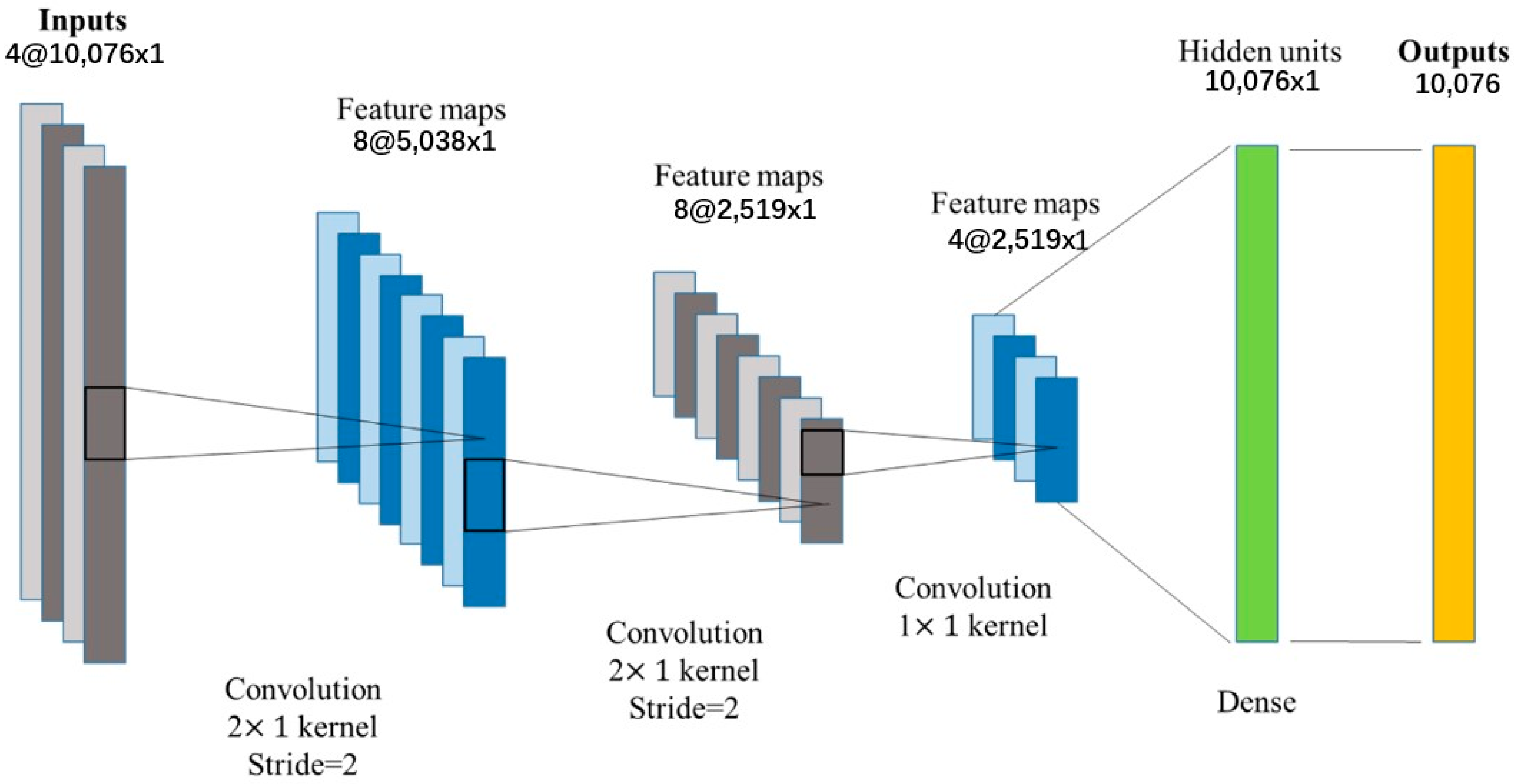
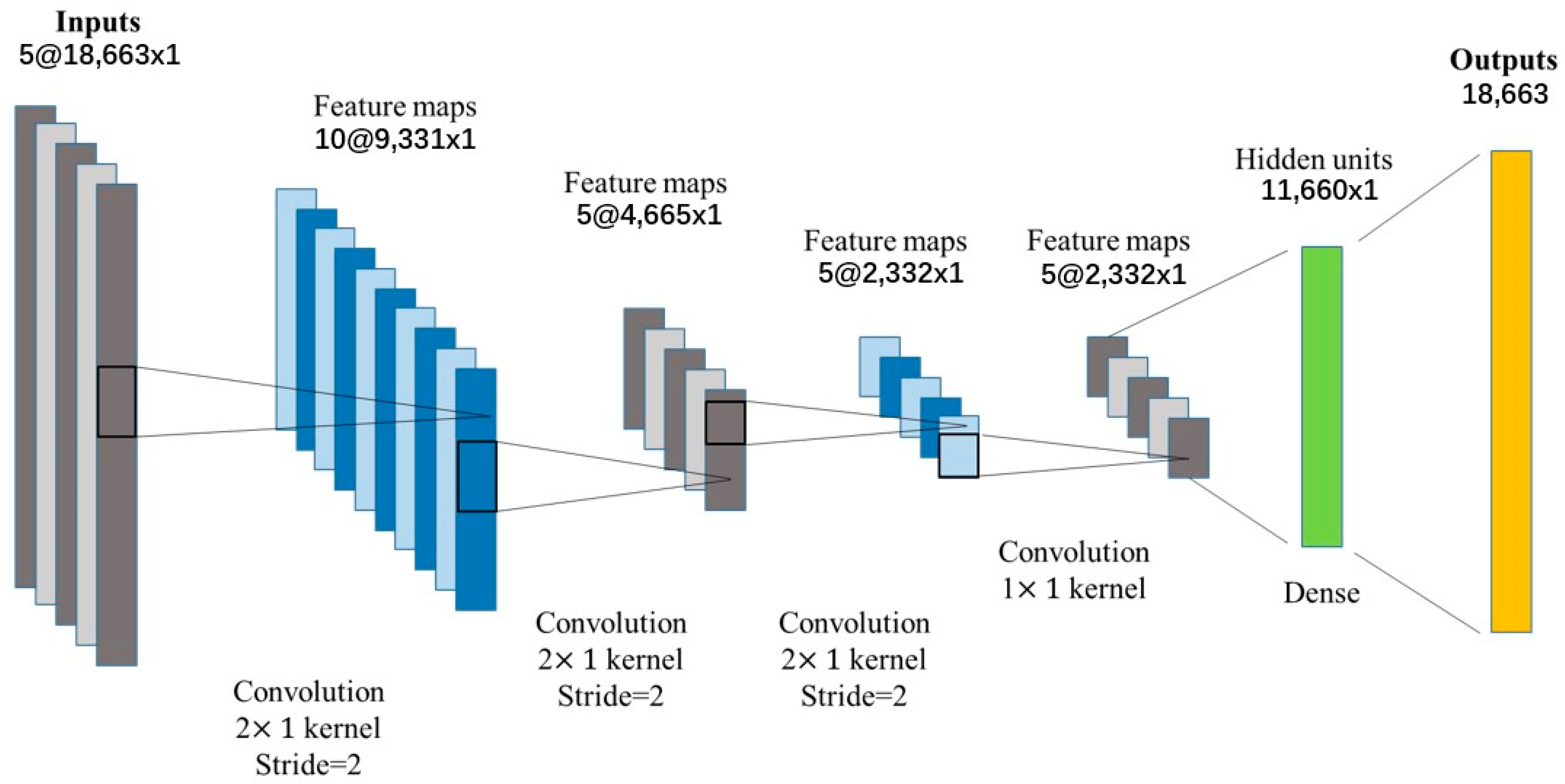
2.2. Artificial Neural Networks

The learning process of artificial neural networks is defined as $N_{l=1}^L$ (α; W, b). This process is established in the analysis of Gaussian processes, where the output of a linear system with a Gaussian distribution as an input is also a Gaussian distribution. By placing Gaussian processes in the displacement function u(x), we obtained Equation (2).

$$\mathit{u}(\mathit{x})\approx GP(0,k(\mathit{x},{\mathit{x}}^{\mathbf{\prime }};\theta )),$$

(2)

where θ is the hyperparameter of the covariance function (k), and GP is the Gaussian process. We assume that all Gaussian process priors used in this process have a squared exponential covariance function without the loss of generality. The Gaussian process provides flexible function priors and is easy to analyze and can be regarded as single-layer feedforward neural network priors with an infinite number of hidden units. Gaussian processes are a type of a method called kernel machines, which are similar to regularization methods. $N_{l=1}^L$ (α; W, b) is a network of L layers. After inputting into the neural network, the weights of the first hidden layer are multiplied, and biases are added, and the obtained data are input into the activation function for processing to obtain the input values of the next layer, as shown in Equation (3).

$$h^l={\mathit{W}}^l\cdot {\mathit{z}}^{l-1}+{\mathit{b}}^l,$$

(3)

where $z^l=o^l(h^l)$. z⁰ and z^L represent the input and output, respectively. W^l and b^l are layer parameters. And $o^l$ denotes an active function.

The mean squared error (MSE) and mean absolute error (MAE) represent the mean sum of squared differences between the predicted values and finite element calculations and the mean absolute difference between the predicted values and finite element calculations, respectively. The mathematical expressions for the MSE and MAE are stated as Equations (4) and (5), respectively.

$$\mathrm{MSE}={\displaystyle \frac{1}{n}}{\displaystyle {\sum }_{j=1}^n{\left(y_j-{\widehat{y}}_j\right)}^2},$$

(4)

$$\mathrm{MAE}={\displaystyle \frac{1}{n}}{\displaystyle {\sum }_{j=1}^n\left|y_j-{\widehat{y}}_j\right|},$$

(5)

where y_j and $\widehat{y_j}$ denote the predicted value and the finite element analytical values, while SMAPE denotes the percentage error rate. The mathematical expression is given as Equation (6).

$$\mathrm{SMAPE}={\displaystyle \frac{1}{n}}{\displaystyle {\sum }_{j=1}^n\left(\frac{\left|y_j-{\widehat{y}}_j\right|}{\left|y_j\right|+\left|{\widehat{y}}_j\right|}\right)\times 100\%}$$

(6)

3. Verifications

As shown in Figure 1, the perforated prestressed simply-supported concrete beam was used to verify the proposed surrogate-based finite element method enhanced by a deep learning technique. This concrete was 5000 mm in length and had a cross-section area of 200 mm × 400 mm, the distance between the two supports was 4600 mm. There were two symmetric open holes that were 400 mm × 160 mm in size along the mid-span of the beam at the belly of the beam, with equal heights of the upper and lower chord members at the opening positions. The size of the openings in the prestressed concrete frame was established with reference to examples in the literature [31,32]. Figure 1a presents the sectional dimensions of the beams and steel bars, and Figure 1b shows the left and right cross-sections of the beams.

In order to balance the accuracy and efficiency of the calculation and to avoid a severe distortion of the mesh around the prestressed steel bars at the beam’s end, the relevant finite element model adopts eight-node hexahedral reduced integral elements (C3D8R) to simulate the concrete part. Ordinary steel bars and prestressed steel bars mainly bear tensile and compressive forces in concrete components, so truss elements (T3D2) are used for simulations. The grid size of the concrete unit was about 40 mm, with 10 grids along the direction of the beam’s height and 5 grids along the direction of the beam’s width. The grid size of the ordinary steel bars and prestressed steel bars was about 80 mm. The finite element model after mesh generation is shown in Figure 2, and the mesh information of every component is shown in

Table 1. The mesh information of every component of the beam.

	Element Style	Number of Elements	Number of Nodes
Concrete	C3D8R	5850	7992
Longitudinal bar	T3D2	750	756
Prestressed bar	T3D2	375	378
Beam stirrup	T3D2	806	806
Chord stirrup	T3D2	144	144
Total	-	7925	10,076

.

In this case, the load, stress, and horizontal position of the opening were changed, which would alter the overall stiffness matrix of the beam. Therefore, the proposed neural network model needs to simultaneously represent multiple global stiffness matrices. A convolutional neural network with four hidden layers was proposed to predict the node displacement, as shown in Figure 3. The first three input channels of a convolutional neural network are the x, y, and z coordinates, while the fourth channel represents the node load of each node. The first hidden layer is a convolutional layer containing 2 convolutional kernels and a ReLU activation function, with a stride of 2. The output feature map size is halved, and the number of output channels is doubled. The second hidden layer is a convolutional layer containing 2 convolutional kernels and a ReLU activation function, with a stride of 2. The output feature map is halved, and the number of input channels is equal to the number of output channels. The third hidden layer is a convolutional layer containing 1 convolution kernel and a ReLU activation function, with a stride of 1. The output feature map has the same size as the input feature map, and the number of output channels is halved. The fourth hidden layer is the flattening layer, which converts a 4-dimensional input into a 2-dimensional output. Finally, the fully connected output layer outputs a total of 10,076 node displacements. The batch-size for neural network training was 256, and the Adam optimizer was used for parameter updates. The loss function was MSE, and the learning rate was set to 0.001. The biases were all 0, and the epochs were 100. Figure 4a,b present MSE and MAE curves represented by arithmetic coordinates.

The stress field prediction results of some samples in the test dataset by the trained neural network are shown in Figure 5, Figure 6, Figure 7, Figure 8 and Figure 9. The stress distributions of von Mises stress values for 10,076 nodes, obtained through neural network predictions and an ABAQUS analysis, are plotted in Gmsh. From this figure, it can be seen that the structural stress distribution predicted by the trained neural network model is almost identical to the finite element analysis results. When training the neural network, it takes approximately 15 min to read the training dataset, test dataset, and all samples for 100 iterations, while using the trained neural network to predict the stress distribution of 2000 samples takes 0.1003 s. Compared to traditional finite element analysis methods, the computational time is greatly reduced. These figures indicate that the error of the proposed neural network model is less than 0.1. Thus, it is demonstrated that the proposed surrogate-based finite element method enhanced by a deep learning technique is efficient and accurate.

In addition, stress concentration refers to the localization of stress in a material, which can exceed the average stress in the material due to geometric discontinuities like holes, notches, or sharp corners. It is essential in designs and analyses to predict the failure, fatigue, and ultimate strength of materials. It has been found that the stress around openings is higher than that of other positions. The stress concentration around openings significantly affects the performance and reliability of engineering components.

4. Numerical Examples

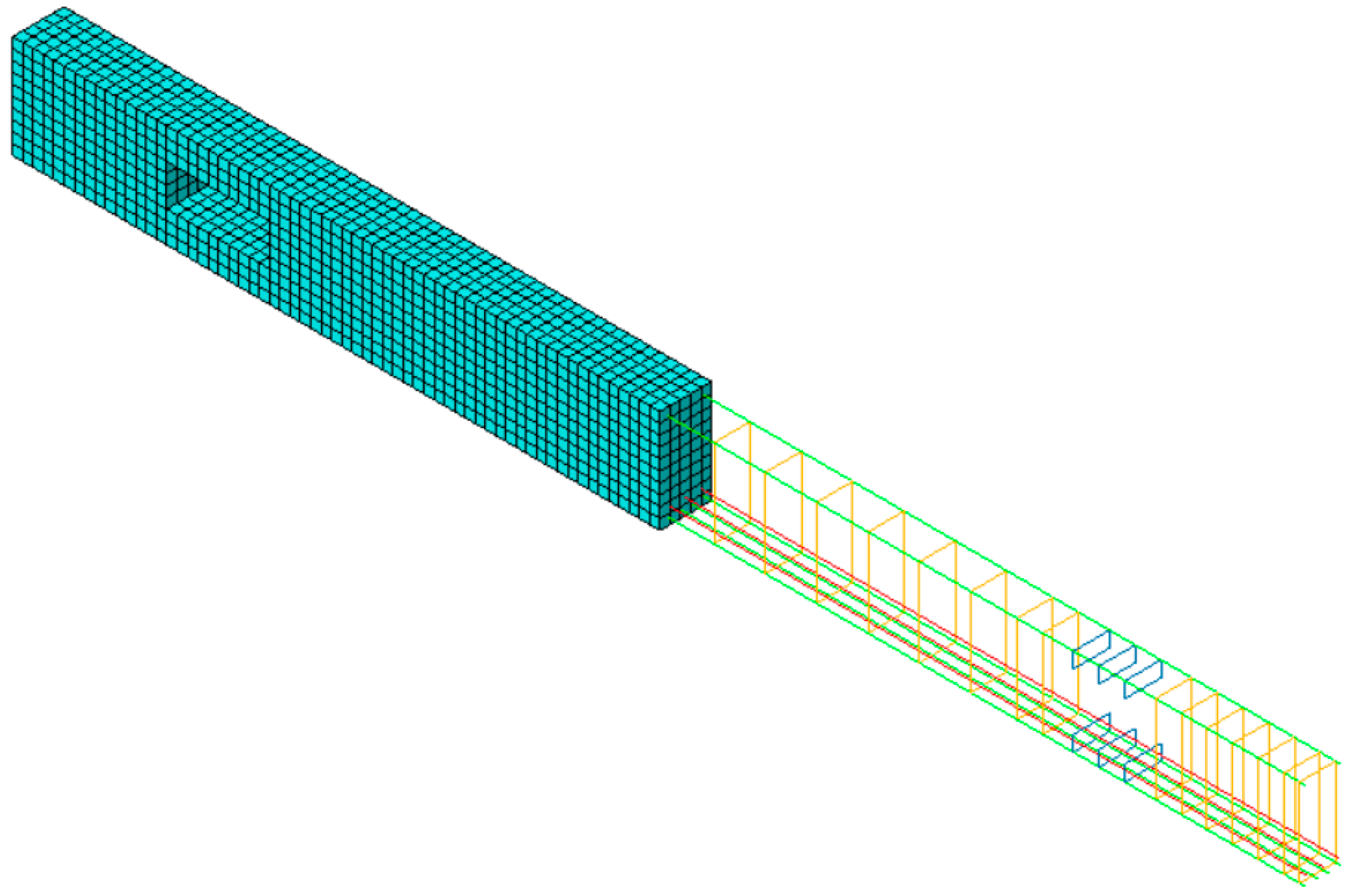
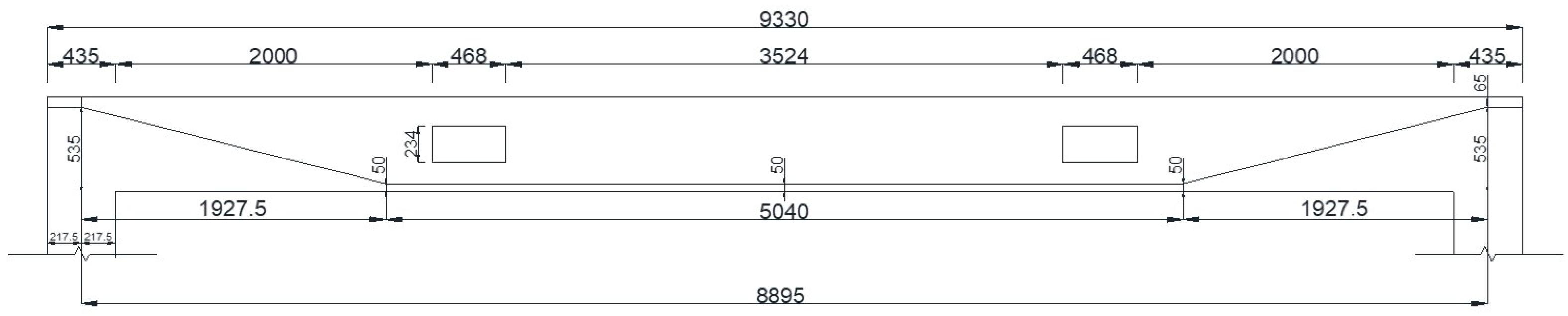
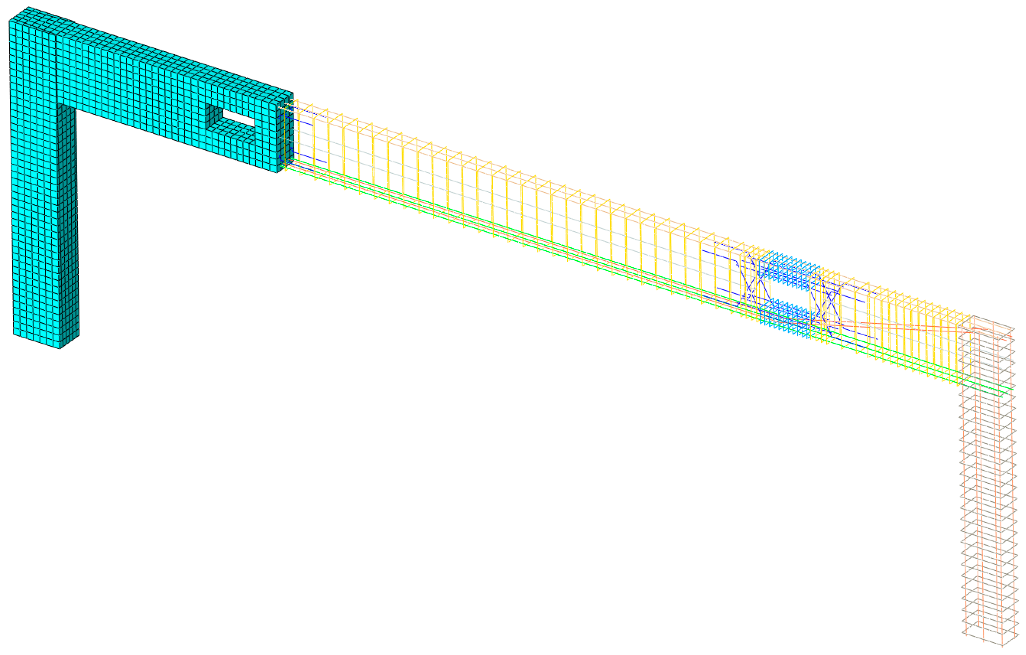
4.1. The Perforated Prestressed Concrete Frame

As shown in Figure 10, Figure 11, Figure 12 and Figure 13, the perforated prestressed concrete frame was analyzed using the proposed surrogate-based finite element method enhanced by a deep learning technique. The prestressed concrete perforated frame had a span width of 8460 mm, was 2770 mm in height, a beam cross-section area of 235 mm × 600 mm, and a column cross-section area of 265 mm × 435 mm. There were two symmetric open holes that were 468 mm × 234 mm in size along the mid-span of the beam at the belly of the beam, with equal heights of the upper and lower chord members at the opening positions. The distance of the openings in the prestressed concrete frame was established with reference to examples in the literature [31,32]. Figure 10 presents the sectional dimensions and steel bars, Figure 11 shows the reinforcement around the opening of the frame, Figure 12 shows the cross-sections of the beam and the column of the frame, and Figure 13 illustrates the layout of the line-shaped prestressed steel bars. The frame dimensions, beam and column sections, position and quantity of column stirrups and longitudinal bars, line type and quantity of prestressing bars, position and quantity of the beam’s longitudinal bars, and position and quantity of the reinforcement around the openings were kept the same. Numerical experiments were made for the frame structures with different opening positions and under different loading conditions.

The relevant finite element model adopts eight-node hexahedral reduced integral elements (C3D8R) to simulate the concrete part. Ordinary steel bars and prestressed steel bars mainly bear tensile and compressive forces in concrete components, so truss elements (T3D2) are used for simulations. The grid size of the concrete unit was about 60 mm, with 10 grids along the direction of the beam’s height, 4 grids along the direction of the beam’s width, 7 grids along the direction of the column’s height, and 6 grids along the direction of the column’s width. The grid size of the ordinary steel bars and prestressed steel bars was about 100 mm. The finite element model after mesh generation is shown in Figure 14, and the mesh information of every component is shown in

Table 2. The mesh information of every component of the frame.

	Element Style	Number of Elements	Number of Nodes
Concrete	C3D8R	9208	12,699
Prestress bar	T3D2	316	318
Beam longitudinal bar	T3D2	465	468
Twisted bar in beam	T3D2	276	282
Beam stirrup	T3D2	1848	1848
Beam chord stirrup	T3D2	440	440
Beam suspension bar	T3D2	264	264
Beam reinforcement bars	T3D2	180	192
Column longitudinal bar	T3D2	552	564
Column stirrup	T3D2	1120	1120
Total	-	15,134	18,663

.

The first three channels of the input of the convolutional neural network were the x, y, and z coordinates of 18,663 nodes, the fourth channel was the node load of each node, and the fifth channel was the reinforcement area of each node. The node area of the concrete unit was set to 0, and the node area of the steel bar unit was inputted according to the actual value. The first hidden layer was a convolutional layer containing 2 convolutional kernels and a ReLU activation function, with a stride of 2. The output feature map size was 9331, and the number of output channels doubled. The second hidden layer was a convolutional layer containing 2 convolutional kernels and a ReLU activation function, with a stride of 2, an output feature map size of 4665, and half of the number of output channels. The third hidden layer was a convolutional layer containing 2 convolutional kernels and a ReLU activation function, with a stride of 2. The output feature map size was 2332, and the number of output channels was equal to the number of input channels. The fourth hidden layer was a convolutional layer containing 1 convolution kernel and a ReLU activation function, with a stride of 1. The output feature map had the same size as the input feature map, and the number of output channels was equal to the number of input channels. The fifth hidden layer was the flattening layer, which converts a 4-dimensional input into a 2-dimensional output. Finally, the fully connected output layer outputted 18,663 node displacements. Figure 15 presents the convolutional neural network with five hidden layers.

The batch size for neural network training was 256, and the Adam optimizer was used for parameter updates. The loss function was the MSE, and the learning rate was set to 0.00005. The biases were all 0, and the epochs were 2000. Figure 16a–c present MSE, MAE, and SMAPE curves in logarithmic coordinates respectively. The results indicate that the proposed neural network can reliably converge. Each sample in this experiment had 18,663 nodes. The time required to read the training dataset, test dataset, and all samples for 2000 iterations when training a neural network was approximately 3 h. The time required to predict the displacement distribution of 5000 samples using the trained neural network was 7.4462 s. The calculation time was significantly reduced compared to traditional finite element analyses.

4.2. Numerical Experiments for Frames with Different Distances between Openings

The concrete stress distributions of the perforated prestressed concrete frames with different distances between the two openings under arbitrarily distributed loading conditions were analyzed using the proposed deep learning technique and the conventional finite element method. Five different opening distances were arbitrarily chosen: 4723 mm, 4124 mm, 3524 mm, 2924 mm, and 2324 mm. Figure 17, Figure 18, Figure 19, Figure 20 and Figure 21 present the stress distribution of the concrete frames with different opening positions using the deep learning technique and the conventional finite element method. These figures indicate that the error of the proposed neural network model is less than 0.1. Thus, it is demonstrated that the proposed surrogate-based finite element method enhanced by a deep learning technique is efficient and accurate.

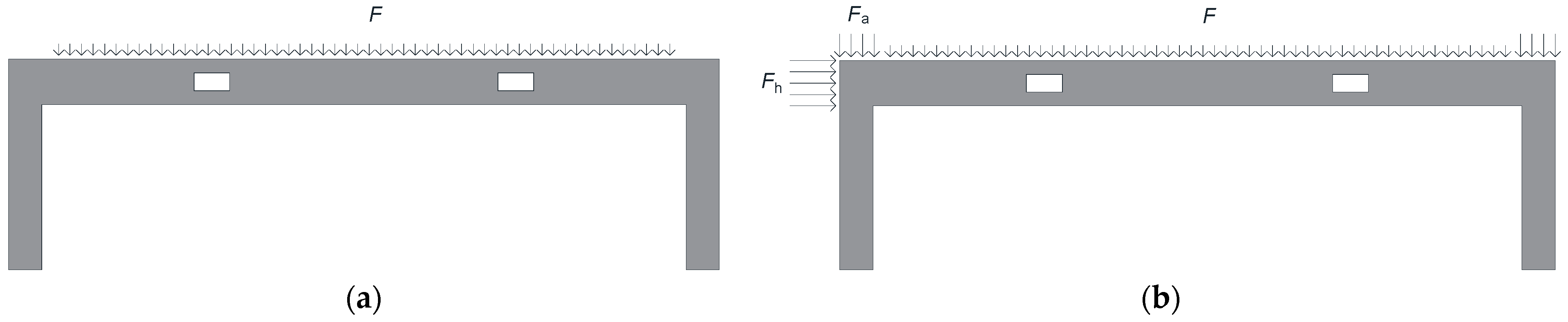
4.3. Numerical Experiments for Perforated Prestressed Concrete under Different Loadings

The vertical and horizontal deflections of the perforated prestressed concrete frames under two different loadings were analyzed using the proposed deep learning technique and the conventional finite element method. Figure 22 presents the two different loadings. Figure 22a shows only a vertical randomly distributed loading on the beam, and Figure 22b expresses both a vertically distributed loading on the beam and a horizontal loading on the top-end area of the left column. Figure 23a presents the vertical deflection of the beam under a vertical randomly distributed loading, and Figure 23b shows the horizontal deflection of the left column under both a vertical arbitrarily distributed loading on the beam and a horizontal loading on the top-end area of the left column. These figures indicate that the error of the proposed neural network model is less than 0.1. Thus, it is demonstrated that the proposed surrogate-based finite element method enhanced by a deep learning technique is efficient and accurate.

This study analyzed prestressed concrete perforated frames at different perforation positions and loading states using deep learning and finite element methods. The proposed convolutional neural network model converges stably during training. When using a training neural network model to predict the displacement and stress fields of a prestressed concrete perforated frame with different opening positions, the errors of stress are less than 5%. When using a training neural network model to predict the displacement and stress fields of a prestressed concrete perforated frame under both horizontal and vertical loadings, the horizontal displacement error is less than 5%, and the stress error is less than 10%. It was shown that the neural network model has high accuracy and can meet engineering requirements. And the computation time is significantly reduced by nearly 50% compared to traditional finite element analyses. It was demonstrated that the efficiency of neural network models is also very high.

5. Conclusions

This study combines machine learning technology with a finite element analysis to study the stress displacement state of prestressed concrete simply supported by beams and frames under a load. The main conclusions are given as follows:

(1)

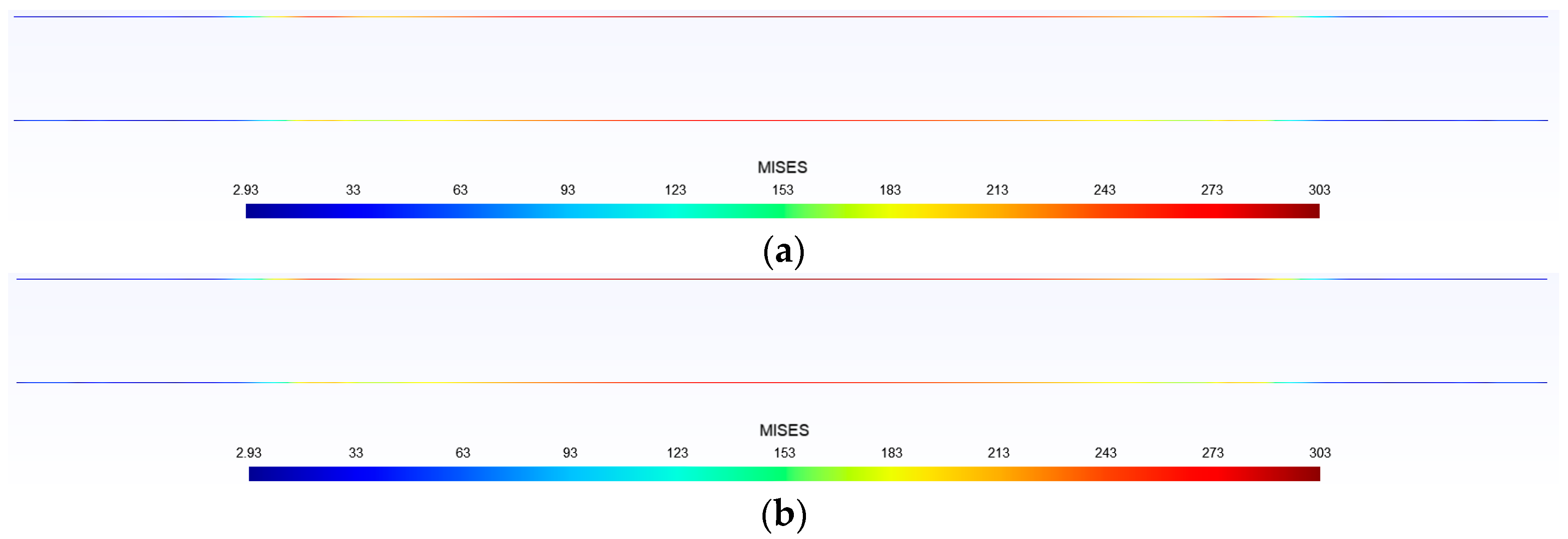
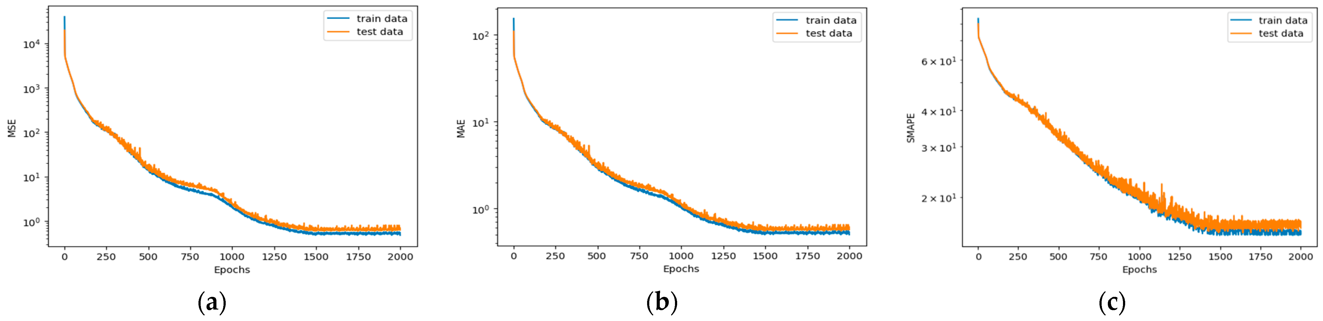
When using a linear regression model to predict the displacement and stress fields of prestressed concrete simply supported by beams with an open hole and a constant total stiffness matrix, the final SMAPE is less than 1%, and the differences in various indicators between the training and testing datasets are small.

(2)

When only changing the opening position, for each type of opening position of the beam, 2000 samples were generated for training by changing the stress levels of each node on the top surface and the tension control stress of the prestressed reinforcement. The SMAPE of the final predicted displacement field and stress field are both less than 5%. When both the opening position and the reinforcement area are changed simultaneously, there is only one sample for each total stiffness matrix. The SMAPE of the final predicted displacement field and stress field is also less than 5%.

(3)

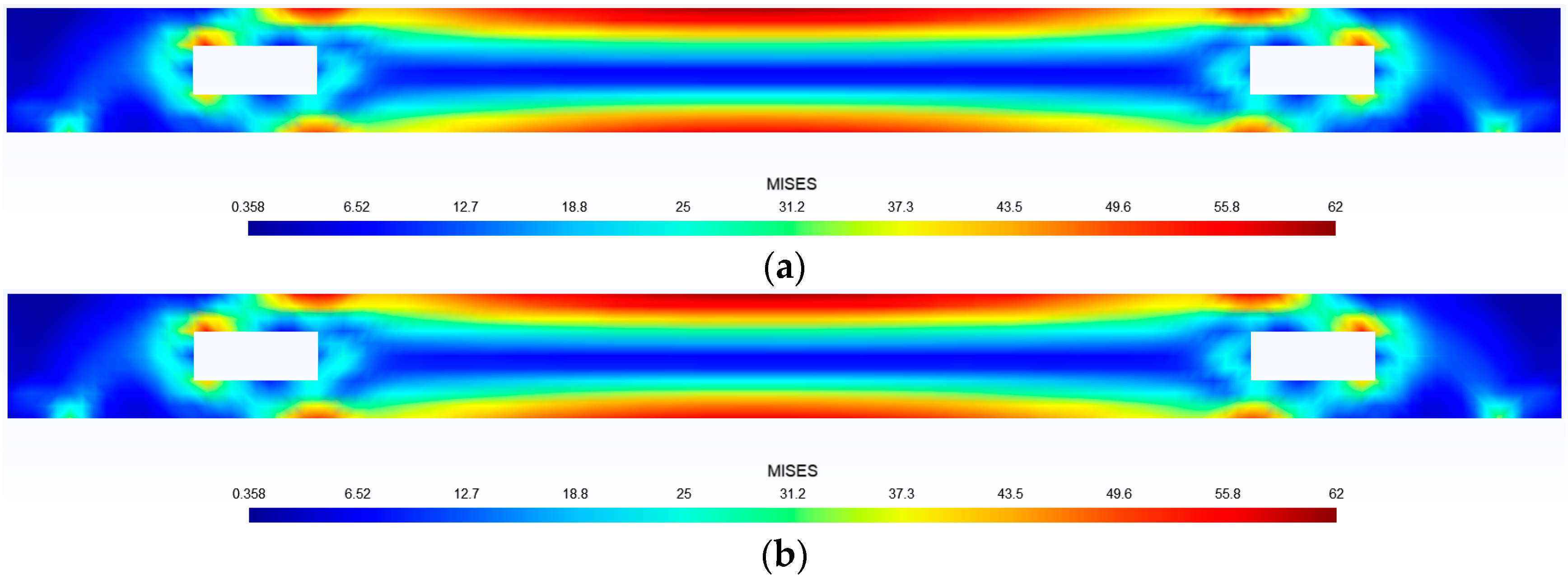
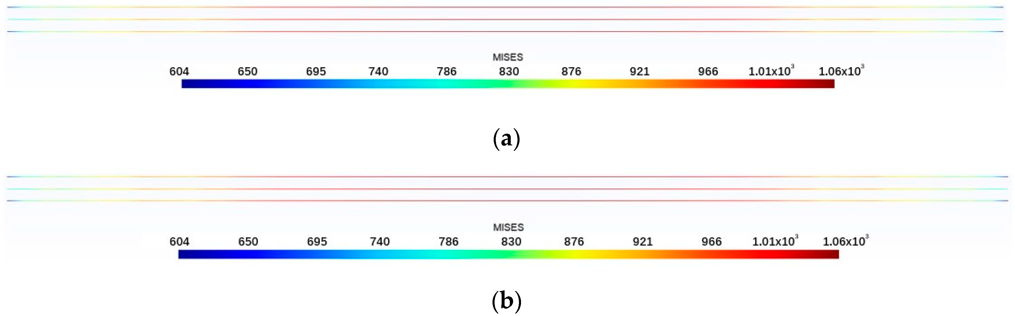
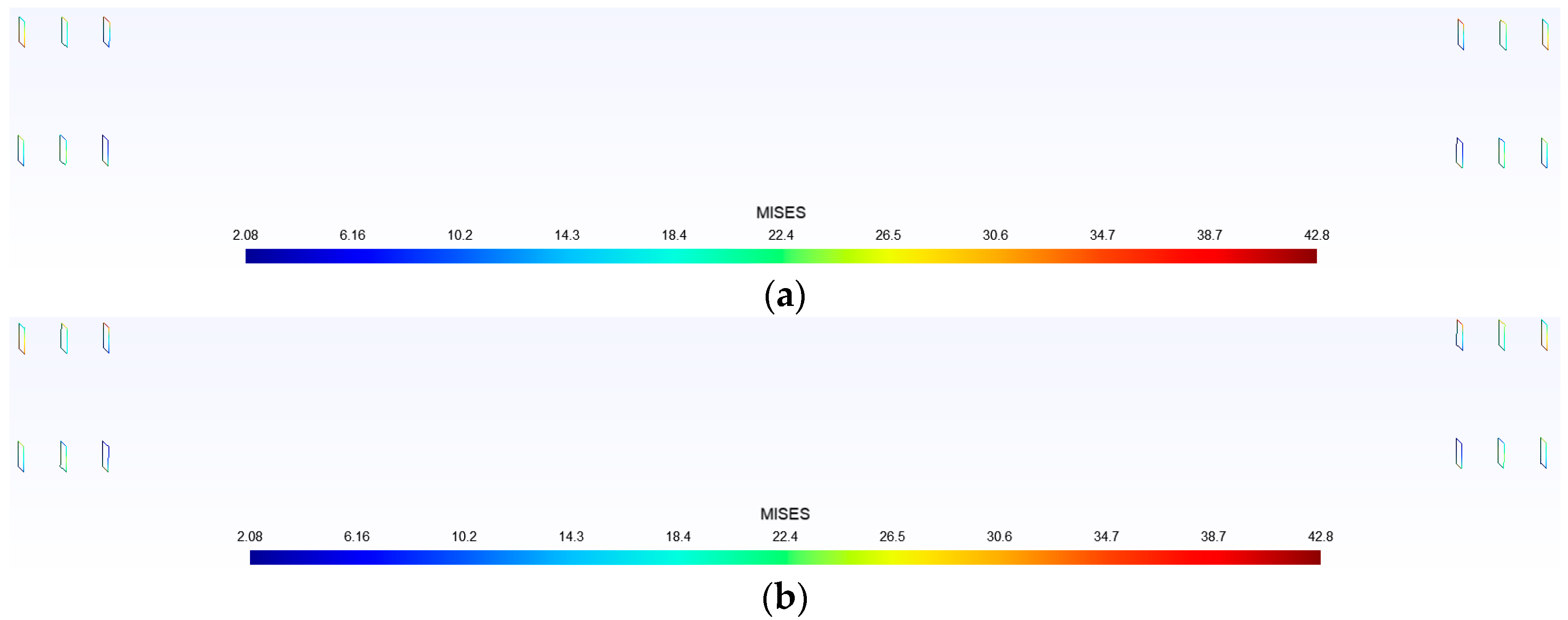
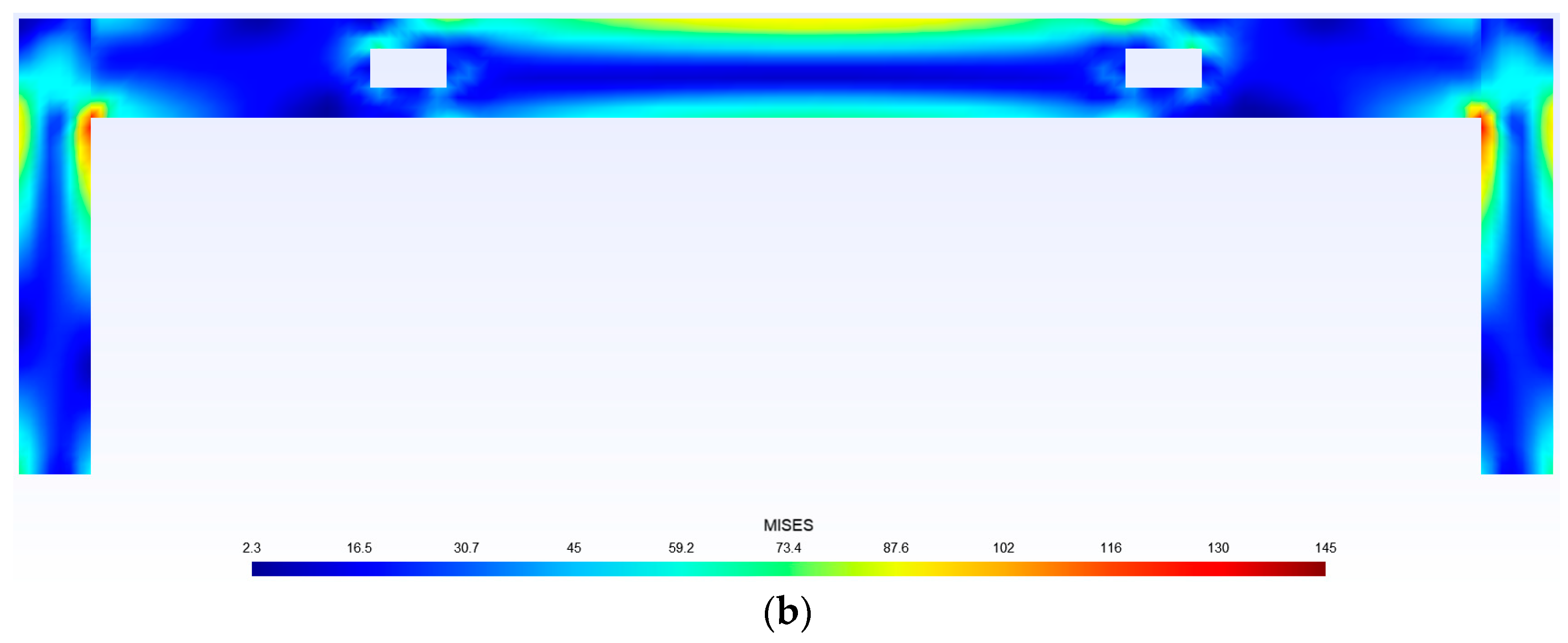
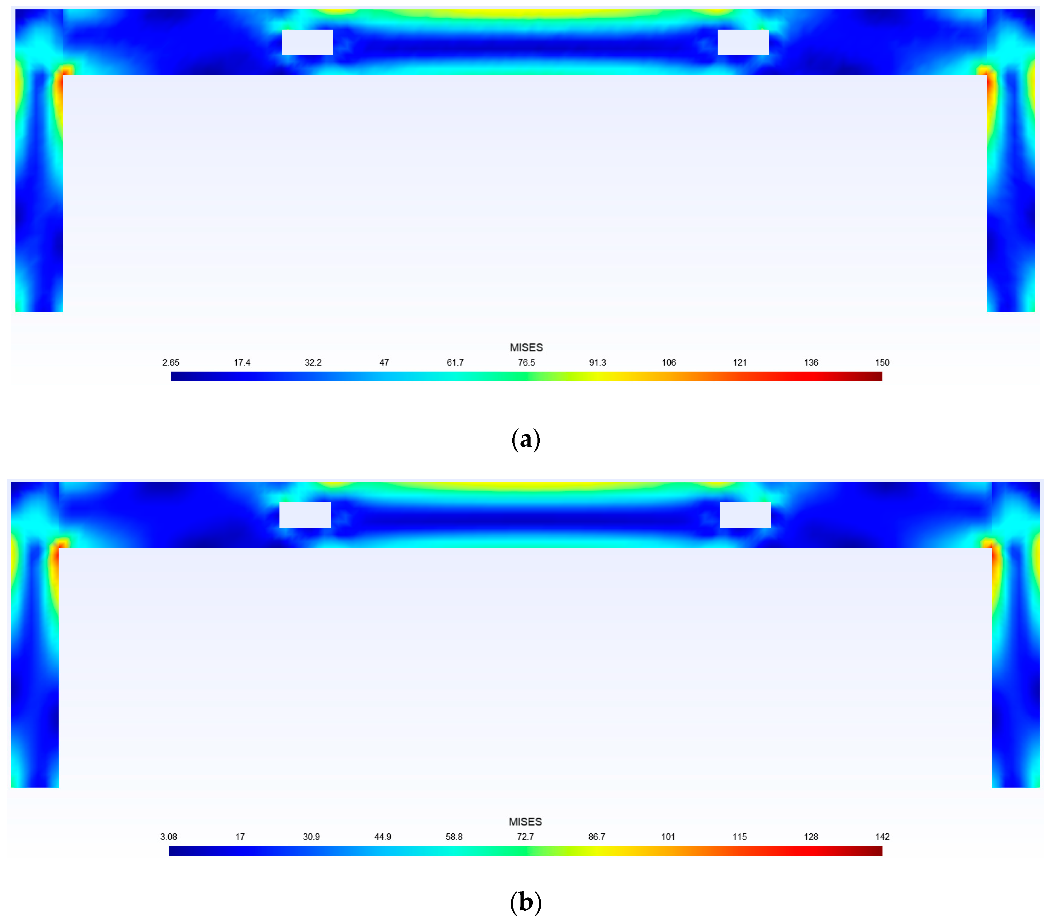
Due to the vertical displacement of each node of the frame column under a vertical load being close to zero, the SMAPE value is relatively high. However, for the vertical displacement field and stress field of the frame beam, the SMAPE is less than 5%, indicating high prediction accuracy.

(4)

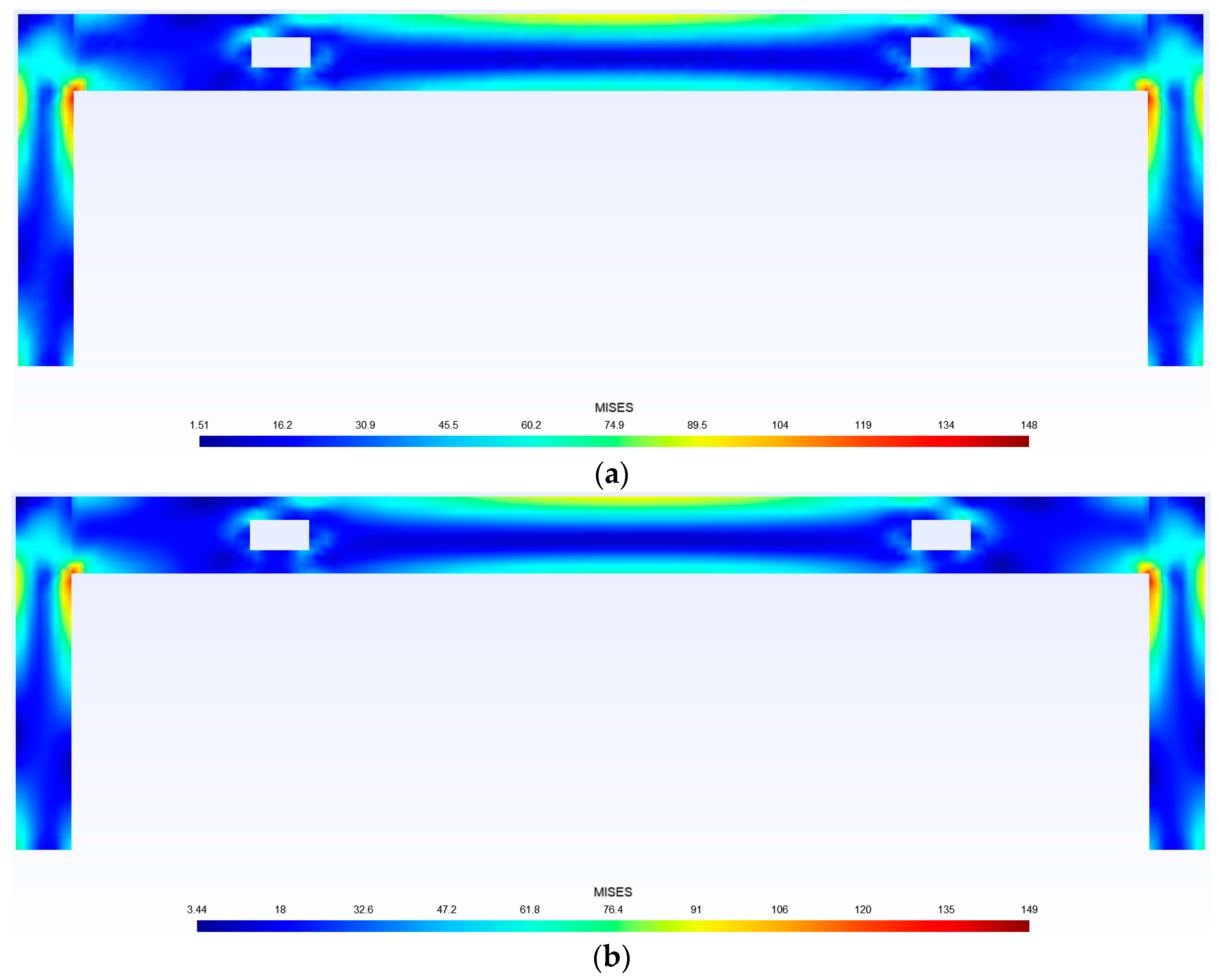
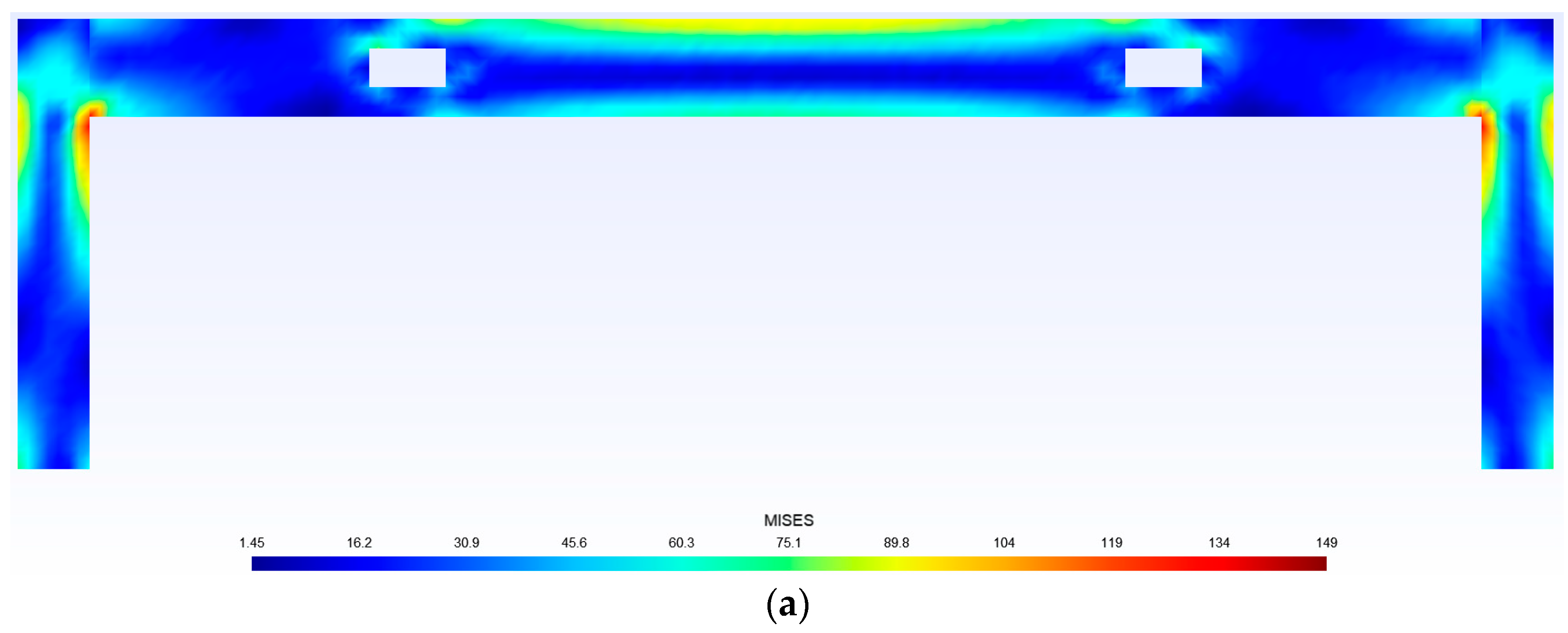
Compared with the results of a finite element analysis, the relative error is larger at areas with lower stress values. However, most cases have a relative error of less than 5% in areas with high stress values. Therefore, it is feasible to use trained deep learning models for predictions.

However, the finite element surrogate analysis method proposed in this article still has room for further refinement in the following areas, which serve as directions for future research. First, to maintain consistency in the number of input and output data for each sample, the number of grids, element types, steel-bar spacing, and quantity for all samples remained unchanged, which is not possible in practical engineering. This is also a difficulty of combining deep learning with finite element simulations. Future work should develop more universal neural network methods that use structures with different numbers of grids for predictions. In addition, all the concrete, steel bars, and prestressed bars in this article were made of linear elastic materials, while in actual engineering, most of them are made of elastic–plastic materials. In the future, researchers should explore how to use deep learning models to analyze the displacement and stress fields of elastic–plastic structures.

References

1. Khatir, A.; Capozucca, R.; Khatir, S.; Magagnini, E. Vibration-based crack prediction on a beam model using hybrid butterfly optimization algorithm with artificial neural network. Front. Struct. Civ. Eng. 2022, 16, 976–989. [Google Scholar] [CrossRef]
2. Teng, S.; Chen, G.; Wang, S.; Zhang, J.; Sun, X. Digital image correlation-based structural state detection through deep learning. Front. Struct. Civ. Eng. 2022, 16, 45–56. [Google Scholar] [CrossRef]
3. Bolandi, H.; Li, X.; Salem, T.; Boddeti, V.N.; Lajnef, N. Bridging finite element and deep learning: High-resolution stress distribution prediction in structural components. Front. Struct. Civ. Eng. 2022, 16, 1365–1377. [Google Scholar] [CrossRef]
4. Lin, M.; Teng, S.; Chen, G.; Lv, J.; Hao, Z. Optimal CNN-based semantic segmentation model of cutting slope images. Front. Struct. Civ. Eng. 2022, 16, 414–433. [Google Scholar] [CrossRef]
5. Mai, H.-V.T.; Nguyen, M.H.; Trinh, S.H.; Ly, H.-B. Optimization of machine learning models for predicting the compressive strength of fiber-reinforced self-compacting concrete. Front. Struct. Civ. Eng. 2023, 17, 284–305. [Google Scholar] [CrossRef]
6. Hai-Bang, L.; Thuy-Anh, N.; Binh, T.P.; May, H.N. A hybrid machine learning model to estimate self-compacting concrete compressive strength. Front. Struct. Civ. Eng. 2022, 16, 990–1002. [Google Scholar]
7. Sun, G.; Shi, J.; Deng, Y. Predicting the capacity of perfobond rib shear connector using an ANN model and GSA method. Front. Struct. Civ. Eng. 2022, 16, 1233–1248. [Google Scholar] [CrossRef]
8. Javanmardi, R.; Ahmadi-Nedushan, B. Optimal design of double-layer barrel vaults using genetic and pattern search algorithms and optimized neural network as surrogate model. Front. Struct. Civ. Eng. 2023, 17, 378–395. [Google Scholar] [CrossRef]
9. Zhi, P.; Wu, Y.C.; Qi, C.; Zhu, T.; Wu, X.; Wu, H.Y. Surrogate-based physics-informed neural networks for elliptic partial differential equations. Mathematics 2023, 11, 2723. [Google Scholar] [CrossRef]
10. Raissi, M.; Perdikaris, P.; Karniadakis, G.E. Physics-informed neural networks: A deep learning framework for solving forward and inverse problems involving nonlinear partial differential equations. J. Comput. Phys. 2018, 378, 686–707. [Google Scholar] [CrossRef]
11. Raissi, M.; Yazdani, A.; Karniadakis, G.E. Hidden fluid mechanics: Learning velocity and pressure fields from flow visual-izations. Science 2020, 367, 1026–1030. [Google Scholar] [CrossRef] [PubMed]
12. Pang, G.; D’elia, M.; Parks, M. nPINNs: Nonlocal physics-informed neural networks for a parametrized nonlocal universal Laplacian operator. Algorithms and applications. J. Comput. Phys. 2020, 422, 109760. [Google Scholar] [CrossRef]
13. Yang, L.; Meng, X.; Karniadakis, G.E. B-PINNs: Bayesian physics-informed neural networks for forward and inverse PDE problems with noisy data. J. Comput. Phys. 2021, 425, 109913. [Google Scholar] [CrossRef]
14. Cui, T.; Fox, C.; O’Sullivan, M.J. Bayesian calibration of a large-scale geothermal reservoir model by a new adaptive delayed acceptance Metropolis Hastings algorithm. Water Resour. Res. 2011, 47, W10521. [Google Scholar] [CrossRef]
15. Jagtap, A.D.; Karniadakis, G.E. Extended physics-informed neural networks (XPINNs): A generalized space-time domain decomposition based deep learning framework for nonlinear partial differential equations. Commun. Comput. Phys. 2021, 28, 2002–2041. [Google Scholar] [CrossRef]
16. Leung, W.T.; Lin, G.; Zhang, Z. NH-PINN: Neural homogenization-based physics-informed neural network for multiscale problems. J. Comput. Phys. 2022, 470, 111539. [Google Scholar] [CrossRef]
17. Chandrasegaran, S.K.; Ramani, K.; Sriram, R.D. The evolution, challenges, and future of knowledge representation in product design systems. Comput.-Aided Des. 2013, 45, 204–228. [Google Scholar] [CrossRef]
18. Fang, J.; Sun, G.; Qiu, N. On design optimization for structural crashworthiness and its state of the art. Struct. Multidiscip. Optim. 2017, 55, 1091–1119. [Google Scholar] [CrossRef]
19. Bhosekar, A.; Ierapetritou, M. Advances in surrogate based modeling, feasibility analysis, and optimization: A review. Comput. Chem. Eng. 2018, 108, 250–267. [Google Scholar] [CrossRef]
20. Schmidt, J.; Marques, M.R.G.; Botti, S. Recent advances and applications of machine learning in solid-state materials science. Comput. Mater. 2019, 5, 83. [Google Scholar] [CrossRef]
21. Abueidda, D.W.; Almasri, M.; Ammourah, R. Prediction and optimization of mechanical properties of composites using convolutional neural networks. Compos. Struct. 2019, 227, 111264. [Google Scholar] [CrossRef]
22. Niekamp, R.; Niemann, J.; Schröder, J. A surrogate model for the prediction of permeabilities and flow through porous media: A machine learning approach based on stochastic Brownian motion. Comput. Mech. 2023, 71, 563–581. [Google Scholar] [CrossRef]
23. Gholizadeh, S.; Seyedpoor, S.M. Shape optimization of arch dams by metaheuristics and neural networks for frequency constraints. Sci. Iran. 2011, 18, 1020–1027. [Google Scholar] [CrossRef]
24. Gholizadeh, S. Performance-based optimum seismic design of steel structures by a modified firefly algorithm and a new neural network. Adv. Eng. Softw. 2015, 81, 50–65. [Google Scholar] [CrossRef]
25. Ranković, V.; Novaković, A.; Grujović, N. Predicting piezometric water level in dams via artificial neural networks. Neural Comput. Appl. 2014, 24, 1115–1121. [Google Scholar] [CrossRef]
26. Liang, L.; Liu, M.; Martin, C. A deep learning approach to estimate stress distribution: A fast and accurate surrogate of finite-element analysis. J. R. Soc. Interface 2018, 15, 20170844. [Google Scholar] [CrossRef]
27. Oishi, A.; Yagawa, G. Computational mechanics enhanced by deep learning. Comput. Methods Appl. Mech. Eng. 2017, 327, 327–351. [Google Scholar] [CrossRef]
28. Kennedy, J.; Abdalla, H. Static response of prestressed girders with openings. J. Struct. Div. Amesican Sociaty Civ. Eng. 1992, 118, 488–504. [Google Scholar] [CrossRef]
29. Abdalla, H.; Kennedy, J. Design against cracking at openings in prestressed concrete beams. J. Prestress. Concr. 1995, 40, 60–75. [Google Scholar] [CrossRef]
30. Abdalla, H.; Kennedy, J.; Fellow, A. Design of prestressed concrete beams with openings. J. Struct. Eng. 1995, 121, 890–898. [Google Scholar] [CrossRef]
31. Cai, J.; Wang, Y.; Chen, Q. Calculation of shear capacity of reinforced concrete simply supported beam with abdominal openings. J. Archit. Struct. 2014, 35, 149–155. (In Chinese) [Google Scholar]
32. Huang, D.; Hou, L.; Cai, J. Experimental study on columns of large steel structure factory buildings with abdominal openings. Ind. Archit. 2012, 42, 128–132. (In Chinese) [Google Scholar]
Figure 1. The perforated prestressed concrete simply supported by beams that was used to verify the proposed surrogate-based finite element method enhanced by a deep learning technique. (a) Sectional dimensions and reinforcement; (b) left and right cross-sections (dimensions: mm).
Buildings 14 03215 g001
Figure 2. The finite element model of the beam after mesh generation.
Buildings 14 03215 g002
Figure 3. The convolutional neural network with four hidden layers.
Buildings 14 03215 g003
Figure 4. (a) MSE and (b) MAE curves represented by arithmetic coordinates.
Buildings 14 03215 g004
Figure 5. Stress distribution of concrete predicted by (a) deep learning models and (b) a finite element analysis (unit: MPa).
Buildings 14 03215 g005
Figure 6. Stress distribution of prestressed bars predicted by (a) deep learning models, and (b) finite element analysis (unit: MPa).
Buildings 14 03215 g006
Figure 7. Stress distribution of longitudinal bars predicted by (a) deep learning models and (b) a finite element analysis (unit: MPa).
Buildings 14 03215 g007
Figure 8. Stress distribution of beam stirrups predicted by (a) deep learning models and (b) a finite element analysis (unit: MPa).
Buildings 14 03215 g008
Figure 9. Stress distribution of chord stirrups predicted by (a) deep learning models and (b) a finite element analysis (unit: MPa).
Buildings 14 03215 g009
Figure 10. Sectional dimensions and steel bars of the perforated prestressed concrete frame.
Buildings 14 03215 g010
Figure 11. Reinforcement around the opening of the frame.
Buildings 14 03215 g011
Figure 12. Reinforcement around the opening of the frame at (a) the middle point of the beam; (b) the opening; (c) the end-point of the beam; and (d) the top of the column.
Buildings 14 03215 g012
Figure 13. Layout of line-shaped prestressed steel bars.
Buildings 14 03215 g013
Figure 14. The finite element model of the frame after mesh generation.
Buildings 14 03215 g014
Figure 15. The convolutional neural network with five hidden layers.
Buildings 14 03215 g015
Figure 16. (a) MSE curve, (b) MAE curve, and (c) SMAPE curve in logarithmic coordinates.
Buildings 14 03215 g016
Figure 17. Stress distribution of concrete with an opening distance of 4724 mm using (a) deep learning models and (b) a finite element analysis (unit: MPa).
Buildings 14 03215 g017
Figure 18. Stress distribution of concrete with an opening distance of 4124 mm using (a) deep learning models and (b) a finite element analysis (unit: MPa).
Buildings 14 03215 g018aBuildings 14 03215 g018b
Figure 19. Stress distribution of concrete with an opening distance of 3524 mm using (a) deep learning models and (b) a finite element analysis (unit: MPa).
Buildings 14 03215 g019
Figure 20. Stress distribution of concrete with an opening distance of 2924 mm using (a) deep learning models and (b) a finite element analysis (unit: MPa).
Buildings 14 03215 g020
Figure 21. Stress distribution of concrete with an opening distance of 2324 mm using (a) deep learning models and (b) a finite element analysis (unit: MPa).
Buildings 14 03215 g021
Figure 22. The perforated prestressed concrete frame with an opening distance of 3524 mm under two different loadings: (a) only a vertical randomly distributed loading on the beam and (b) both a vertically distributed loading on the beam and a horizontal loading on the top-end area of the left column.
Buildings 14 03215 g022
Figure 23. (a) Vertical deflection of the beam under a vertical randomly distributed loading and (b) horizontal deflection of the left column under both a vertical arbitrarily distributed loading on the beam and a horizontal loading on the top-end area of the left column.
Buildings 14 03215 g023