
Advancing Efficiency in Mineral Construction Materials Recycling: A Comprehensive Approach Integrating Machine Learning and X-ray Diffraction Analysis


Abstract
1. Introduction
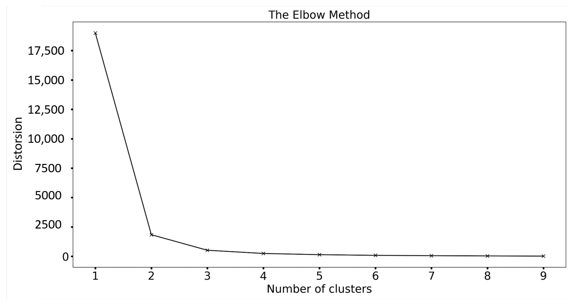
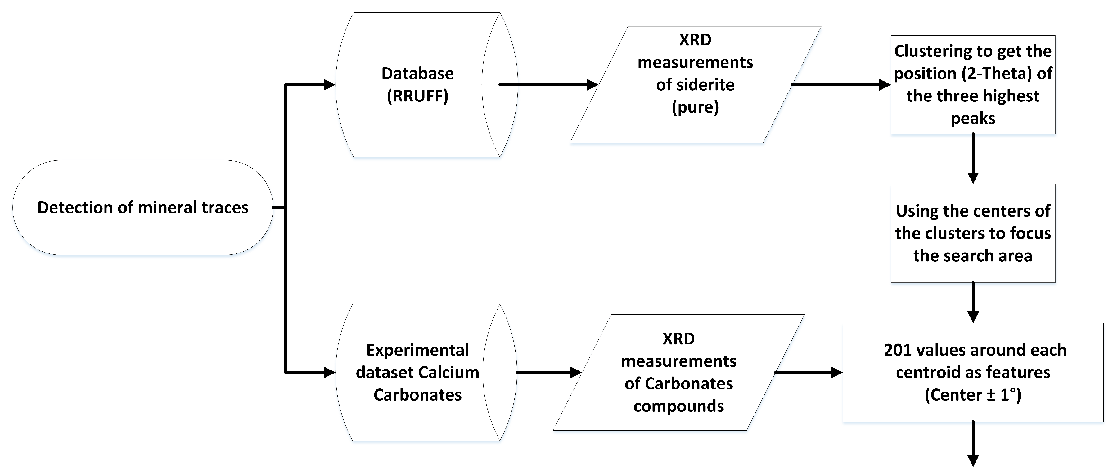
- Obtain pure measurements of the target mineral from the database and cluster the highest peaks.
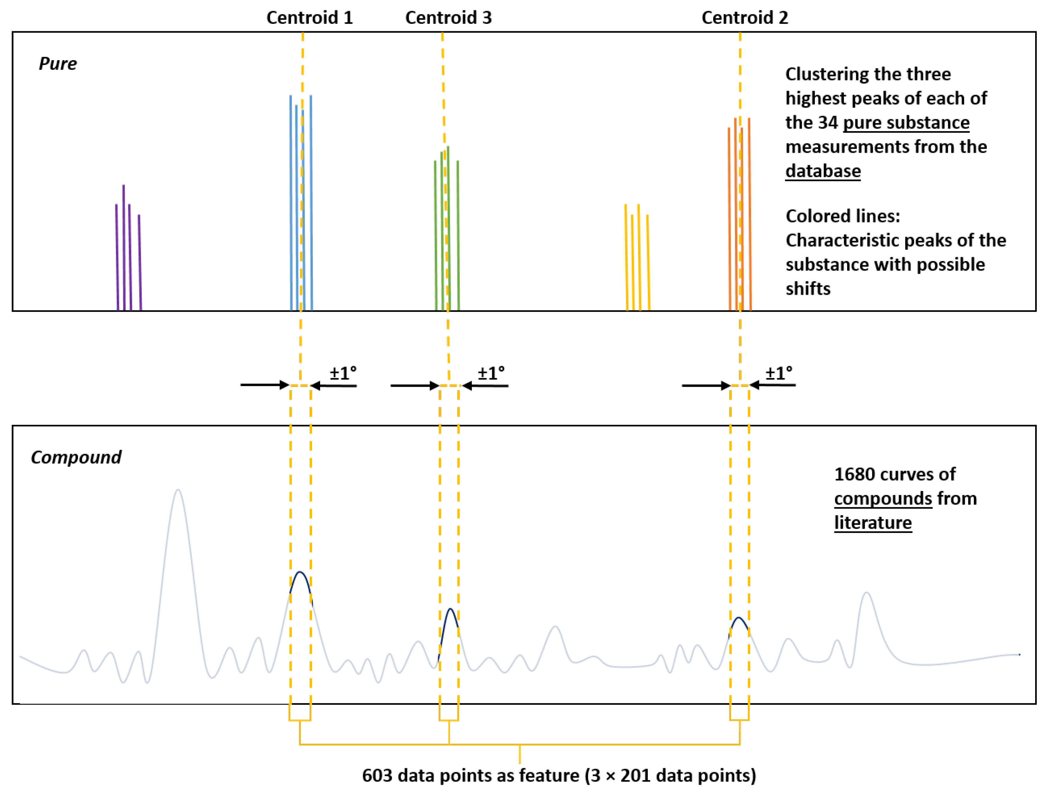
- Utilize these peaks to define a data region from which information can be extracted for training and prediction from compound measurements.
- Train and test a machine learning model to detect traces of the target mineral.
2. Literature Review

| Authors | Year | Algorithm | Target |
|---|---|---|---|
| Bunn et al. [12] | 2015 | ADA boost | Phase identification |
| Bunn et al. [13] | 2016 | k-means, experts | Phase identification |
| Park et al. [2] | 2017 | CNN | Space-group, extinction-group, crystal-system |
| Ryan et al. [3] | 2018 | DNN | Crystal structure |
| Vecsei et al. [5] | 2019 | DNN, CNN | Space-group, crystal-system |
| Oviedo et al. [6] | 2019 | Naive Bayes, kNN, logistic regression, RF, DT, SVM, gradient boosting regression trees, fully connected DNN, a-CNN, DTW + kNN classification. | Space-group, crystal dimensionality |
| Utimula et al. [4] | 2020 | DTW | Concentration of substituents |
| Lee et al. [7] | 2020 | CNN, kNN, RF, SVM | Phase identification |
| Wang et al. [8] | 2020 | CNN | Identification of XRD patterns |
| Dong et al. [9] | 2021 | CNN | Scale factor, lattice parameter, crystallite size maps |
| Szymanski et al. [10] | 2021 | CNN, branching algorithm | Phase identification |
| Szymanski et al. [11] | 2023 | CNN-guided measurement, RF | Phase identification |
| Yanxon et al. [14] | 2023 | kNN, extra tree, gradient boosting, RF | Single-crystal diffraction spots |
3. X-ray Diffraction in Mineralogy
4. Methods and Data
4.1. Data Preparation
4.2. Machine Learning Model
5. Discussion and Further Research
6. Conclusions
- Objective: Develop a machine learning approach for detecting mineral traces in XRD-analyzed mixtures.
- Data source: Use of pure substance measurements for the searched mineral (siderite) from a relevant database and 1680 measurements of carbonate compounds for training and testing.
- Feature Extraction: Extract the highest points from each pure substance measurement and cluster them, resulting in centroids. The intensities extracted from 1680 measurements around the mean 2-theta values serve as characteristics for training and testing.
- Machine learning method: Random forest (RF) was chosen, achieving an 83% accuracy in training. A randomized search was employed for parameter tuning, and five-fold cross-validation was used for validation.
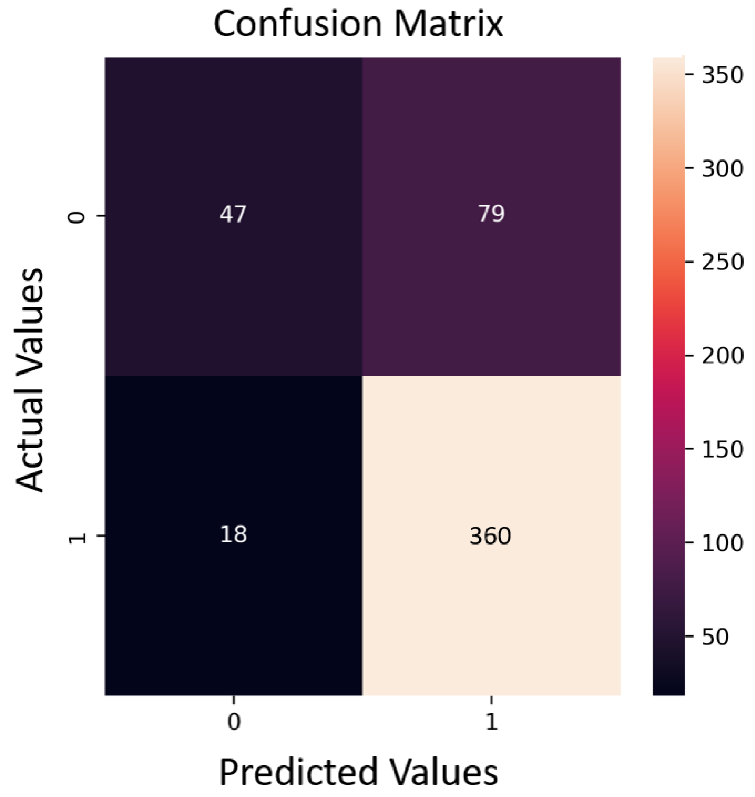
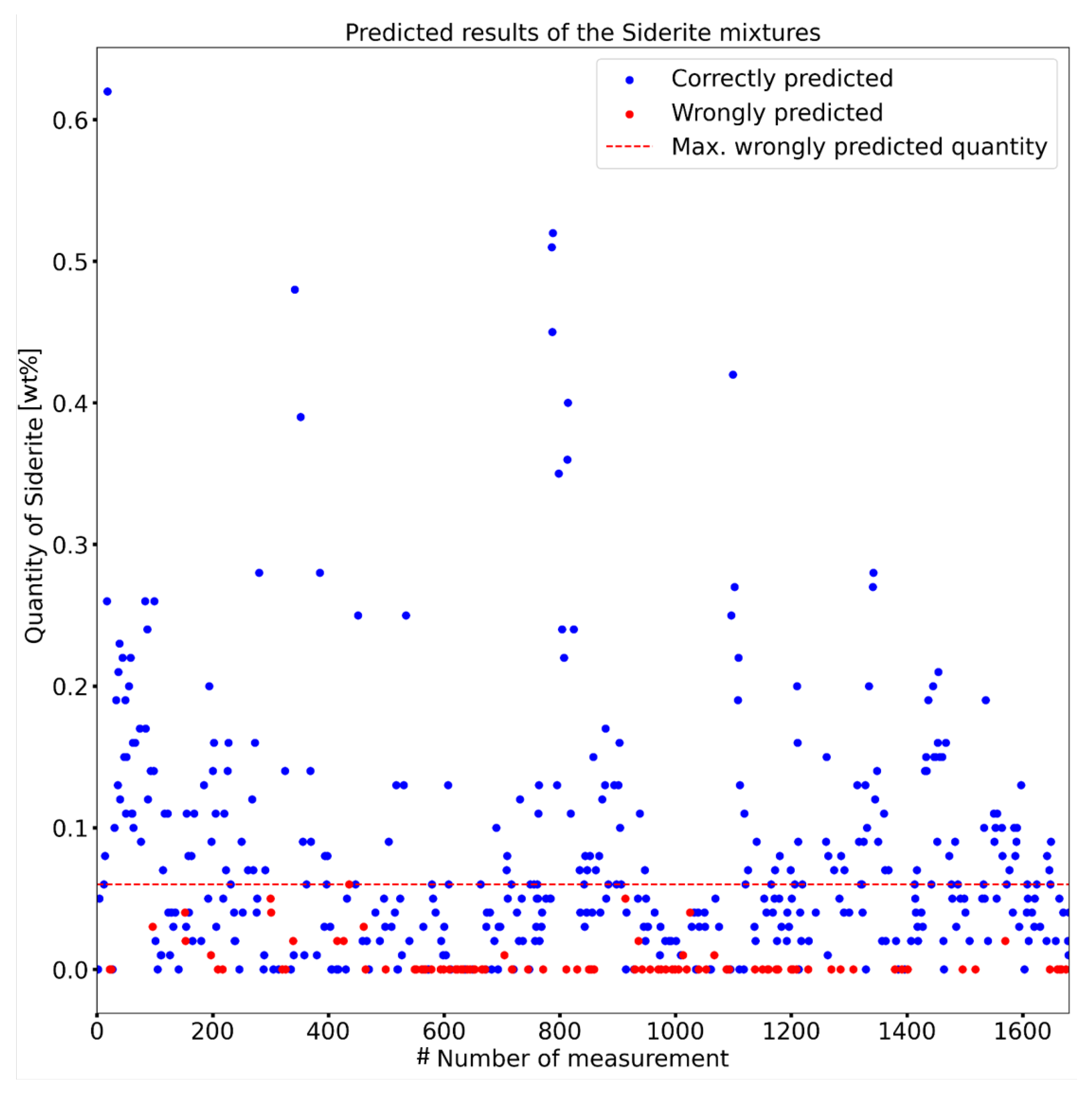
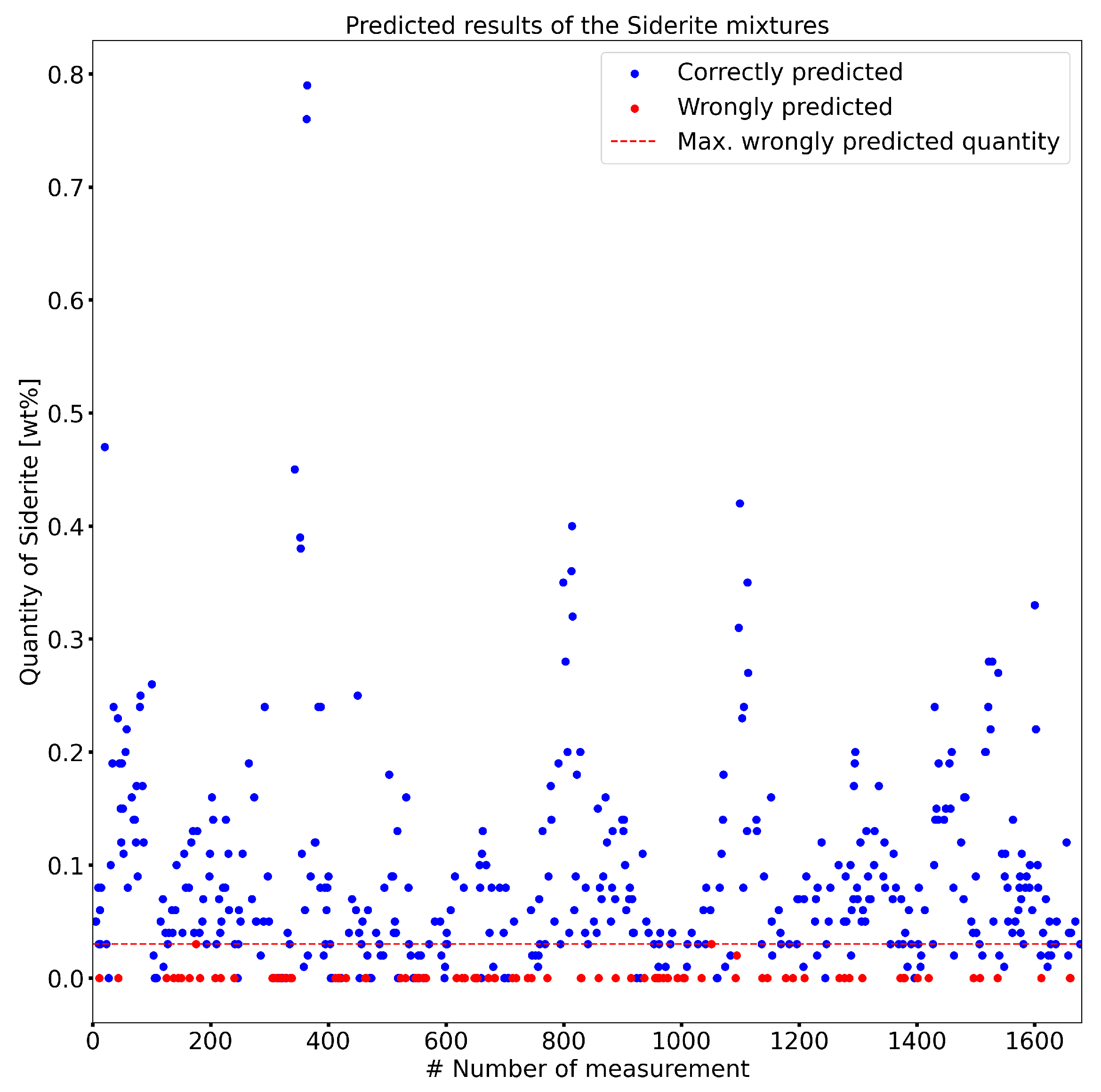
- Results: An 81% accuracy was achieved in predicting test data. No prediction errors were observed above 0.06 wt% of siderite content in the compounds.
Author Contributions
Funding
Data Availability Statement
Acknowledgments
Conflicts of Interest
Abbreviations
| a-CNN | all-Convolutional Neural Network |
| CNN | Convolutional Neural Network |
| DNN | Deep Neural Network |
| DT | Decision Tree |
| DTW | Dynamic Time Warping |
| fn | false negatives |
| fp | false positives |
| kNN | k-Nearest Neighbor |
| NN | Neural Network |
| RF | Random Forest |
| SVM | Support Vector Machine |
| tp | true positives |
| wt% | mass fraction in % |
| XRD | X-ray powder diffraction |
References
- Papamichael, I.; Voukkali, I.; Loizia, P.; Zorpas, A.A. Construction and demolition waste framework of circular economy: A mini review. Waste Manag. Res. 2023, 41, 1728–1740. [Google Scholar] [CrossRef] [PubMed]
- Park, W.B.; Chung, J.; Jung, J.; Sohn, K.; Singh, S.P.; Pyo, M.; Shin, N.; Sohn, K.S. Classification of crystal structure using a convolutional neural network. IUCrJ 2017, 4, 486–494. [Google Scholar] [CrossRef] [PubMed]
- Ryan, K.; Lengyel, J.; Shatruk, M. Crystal structure prediction via deep learning. J. Am. Chem. Soc. 2018, 140, 10158–10168. [Google Scholar] [CrossRef] [PubMed]
- Utimula, K.; Hunkao, R.; Yano, M.; Kimoto, H.; Hongo, K.; Kawaguchi, S.; Suwanna, S.; Maezono, R. Machine-Learning Clustering Technique Applied to Powder X-Ray Diffraction Patterns to Distinguish Compositions of ThMn12-Type Alloys. Adv. Theory Simul. 2020, 3, 2000039. [Google Scholar] [CrossRef]
- Vecsei, P.M.; Choo, K.; Chang, J.; Neupert, T. Neural network based classification of crystal symmetries from x-ray diffraction patterns. Phys. Rev. B 2019, 99, 245120. [Google Scholar] [CrossRef]
- Oviedo, F.; Ren, Z.; Sun, S.; Settens, C.; Liu, Z.; Hartono, N.T.P.; Ramasamy, S.; DeCost, B.L.; Tian, S.I.; Romano, G.; et al. Fast and interpretable classification of small X-ray diffraction datasets using data augmentation and deep neural networks. NPJ Comput. Mater. 2019, 5, 60. [Google Scholar] [CrossRef]
- Lee, J.W.; Park, W.B.; Lee, J.H.; Singh, S.P.; Sohn, K.S. A deep-learning technique for phase identification in multiphase inorganic compounds using synthetic XRD powder patterns. Nat. Commun. 2020, 11, 86. [Google Scholar] [CrossRef] [PubMed]
- Wang, H.; Xie, Y.; Li, D.; Deng, H.; Zhao, Y.; Xin, M.; Lin, J. Rapid identification of X-ray diffraction patterns based on very limited data by interpretable convolutional neural networks. J. Chem. Inf. Model. 2020, 60, 2004–2011. [Google Scholar] [CrossRef]
- Dong, H.; Butler, K.T.; Matras, D.; Price, S.W.; Odarchenko, Y.; Khatry, R.; Thompson, A.; Middelkoop, V.; Jacques, S.D.; Beale, A.M.; et al. A deep convolutional neural network for real-time full profile analysis of big powder diffraction data. NPJ Comput. Mater. 2021, 7, 74. [Google Scholar] [CrossRef]
- Szymanski, N.J.; Bartel, C.J.; Zeng, Y.; Tu, Q.; Ceder, G. Probabilistic deep learning approach to automate the interpretation of multi-phase diffraction spectra. Chem. Mater. 2021, 33, 4204–4215. [Google Scholar] [CrossRef]
- Szymanski, N.J.; Bartel, C.J.; Zeng, Y.; Diallo, M.; Kim, H.; Ceder, G. Adaptively driven X-ray diffraction guided by machine learning for autonomous phase identification. NPJ Comput. Mater. 2023, 9, 31. [Google Scholar] [CrossRef]
- Bunn, J.K.; Han, S.; Zhang, Y.; Tong, Y.; Hu, J.; Hattrick-Simpers, J.R. Generalized machine learning technique for automatic phase attribution in time variant high-throughput experimental studies. J. Mater. Res. 2015, 30, 879–889. [Google Scholar] [CrossRef]
- Bunn, J.K.; Hu, J.; Hattrick-Simpers, J.R. Semi-supervised approach to phase identification from combinatorial sample diffraction patterns. Jom 2016, 68, 2116–2125. [Google Scholar] [CrossRef]
- Yanxon, H.; Weng, J.; Parraga, H.; Xu, W.; Ruett, U.; Schwarz, N. Artifact identification in X-ray diffraction data using machine learning methods. J. Synchrotron Radiat. 2023, 30, 137–146. [Google Scholar] [CrossRef] [PubMed]
- Lafuente, B.; Downs, R.T.; Yang, H.; Stone, N. The power of databases: The RRUFF project. Highlights Mineral. Crystallogr. 2015, 1, 25. [Google Scholar] [CrossRef]
- Thorndike, R.L. Who belongs in the family? Psychometrika 1953, 18, 267–276. [Google Scholar] [CrossRef]
- Yuan, C.; Yang, H. Research on K-value selection method of K-means clustering algorithm. J 2019, 2, 226–235. [Google Scholar] [CrossRef]
- Lavina, B.; Dera, P.; Downs, R.T.; Yang, W.; Sinogeikin, S.; Meng, Y.; Shen, G.; Schiferl, D. Structure of siderite FeCO3 to 56 GPa and hysteresis of its spin-pairing transition. Phys. Rev. B 2010, 82, 064110. [Google Scholar] [CrossRef]
- Amao, A.O.; Al-Otaibi, B.; Al-Ramadan, K. High-resolution X–ray diffraction datasets: Carbonates. Data Brief 2022, 42, 108204. [Google Scholar] [CrossRef] [PubMed]
- Pedregosa, F.; Varoquaux, G.; Gramfort, A.; Michel, V.; Thirion, B.; Grisel, O.; Blondel, M.; Prettenhofer, P.; Weiss, R.; Dubourg, V.; et al. Scikit-learn: Machine Learning in Python. J. Mach. Learn. Res. 2011, 12, 2825–2830. [Google Scholar]


| Mineral | Crystal System | Unit Cell |
|---|---|---|
| Siderite | trigonal | |
| space group Rc | Å; Å | |
| Calcite | trigonal | |
| space group Rc | Å; Å | |
| High-Mg calcite | trigonal | |
| space group Rc | Å; Å | |
| Vaterite | hexagonal | |
| space group P/mmc | Å; Å | |
| Smithonite | trigonal | |
| space group Rc | Å; Å | |
| Rhodochrosite | trigonal | |
| space group Rc | Å; Å | |
| Dolomite | trigonal | |
| space group R | Å; Å | |
| Monohydrocalcite | trigonal | |
| space group P | Å; Å | |
| Otavite | trigonal | |
| space group R | Å; Å |
| Hyper-Parameter | |||
|---|---|---|---|
| n_estimators | start = 10 | end = 2000 | num = 30 |
| max_features | sqrt | ||
| max_depth | start = 10 | end = 200 | num = 20 |
| min_sample_leaf | 1 | 2 | 4 |
| bootstrap | True | False | |
| criterion | gini | entropy |
| Precision | Recall | F1 -Score | Support | |
|---|---|---|---|---|
| Devoid of siderite | 0.72 | 0.37 | 0.49 | 126 |
| Containing siderite | 0.82 | 0.95 | 0.88 | 378 |
| Accuracy | 0.81 | 504 | ||
| Macro average | 0.77 | 0.66 | 0.69 | 504 |
| Weighted average | 0.80 | 0.81 | 0.78 | 504 |
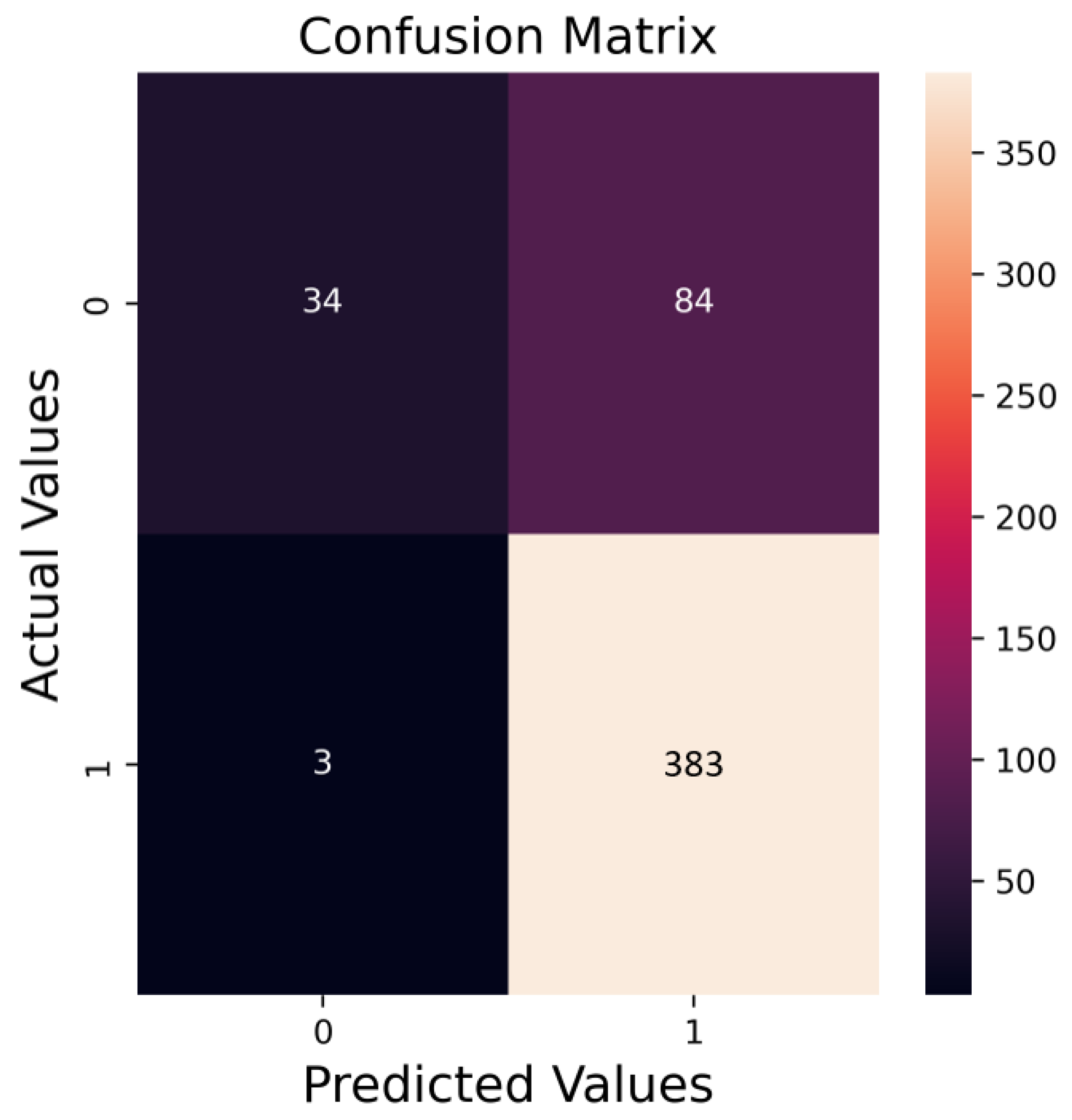
| Precision | Recall | F1 -Score | Support | |
|---|---|---|---|---|
| Devoid of siderite | 0.92 | 0.29 | 0.44 | 118 |
| Containing siderite | 0.82 | 0.99 | 0.90 | 386 |
| Accuracy | 0.83 | 504 | ||
| Macro average | 0.87 | 0.64 | 0.67 | 504 |
| Weighted average | 0.84 | 0.83 | 0.79 | 504 |
Disclaimer/Publisher’s Note: The statements, opinions and data contained in all publications are solely those of the individual author(s) and contributor(s) and not of MDPI and/or the editor(s). MDPI and/or the editor(s) disclaim responsibility for any injury to people or property resulting from any ideas, methods, instructions or products referred to in the content. |
© 2024 by the authors. Licensee MDPI, Basel, Switzerland. This article is an open access article distributed under the terms and conditions of the Creative Commons Attribution (CC BY) license (https://creativecommons.org/licenses/by/4.0/).
Share and Cite
Wilhelm, M.; Lotter, F.; Scherdel, C.; Schmitt, J. Advancing Efficiency in Mineral Construction Materials Recycling: A Comprehensive Approach Integrating Machine Learning and X-ray Diffraction Analysis. Buildings 2024, 14, 340. https://doi.org/10.3390/buildings14020340
Wilhelm M, Lotter F, Scherdel C, Schmitt J. Advancing Efficiency in Mineral Construction Materials Recycling: A Comprehensive Approach Integrating Machine Learning and X-ray Diffraction Analysis. Buildings. 2024; 14(2):340. https://doi.org/10.3390/buildings14020340
Chicago/Turabian StyleWilhelm, Markus, Frank Lotter, Christian Scherdel, and Jan Schmitt. 2024. "Advancing Efficiency in Mineral Construction Materials Recycling: A Comprehensive Approach Integrating Machine Learning and X-ray Diffraction Analysis" Buildings 14, no. 2: 340. https://doi.org/10.3390/buildings14020340
APA StyleWilhelm, M., Lotter, F., Scherdel, C., & Schmitt, J. (2024). Advancing Efficiency in Mineral Construction Materials Recycling: A Comprehensive Approach Integrating Machine Learning and X-ray Diffraction Analysis. Buildings, 14(2), 340. https://doi.org/10.3390/buildings14020340