
Bridge Construction Risk Assessment Based on Variable Weight Theory and Cloud Model

Abstract
:1. Introduction
2. Research Theory
2.1. Variable Weight Theory
- (1)
- Let , if , then is monotonically decreasing. If , then is monotonically increasing.
- (2)
- Let , if , then is monotonically decreasing. If , then is monotonically increasing and satisfies the continuity condition.
- (3)
- For any fixed weight vector , Equation (1) is satisfied.
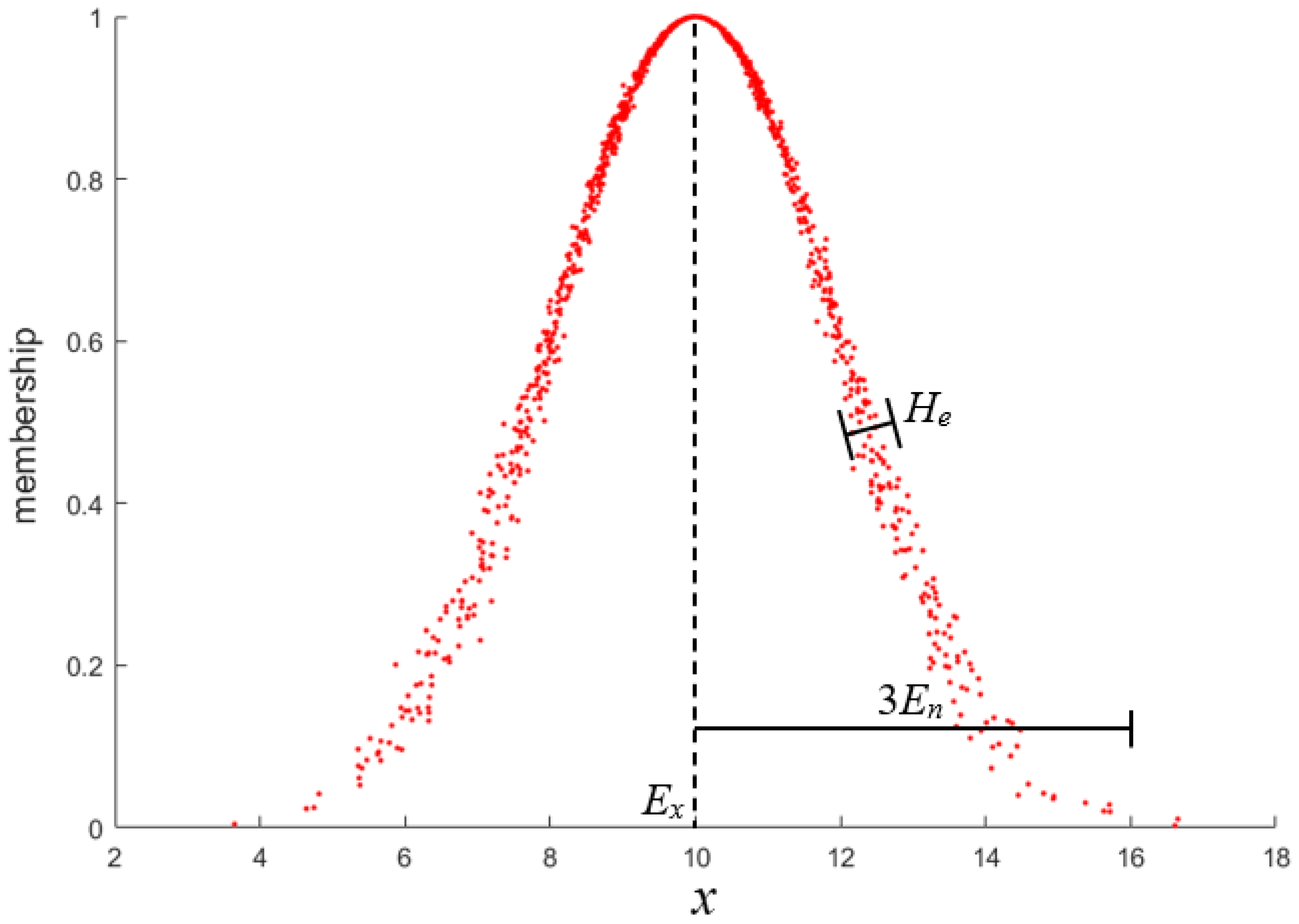
2.2. Cloud Model
2.3. IFAHP
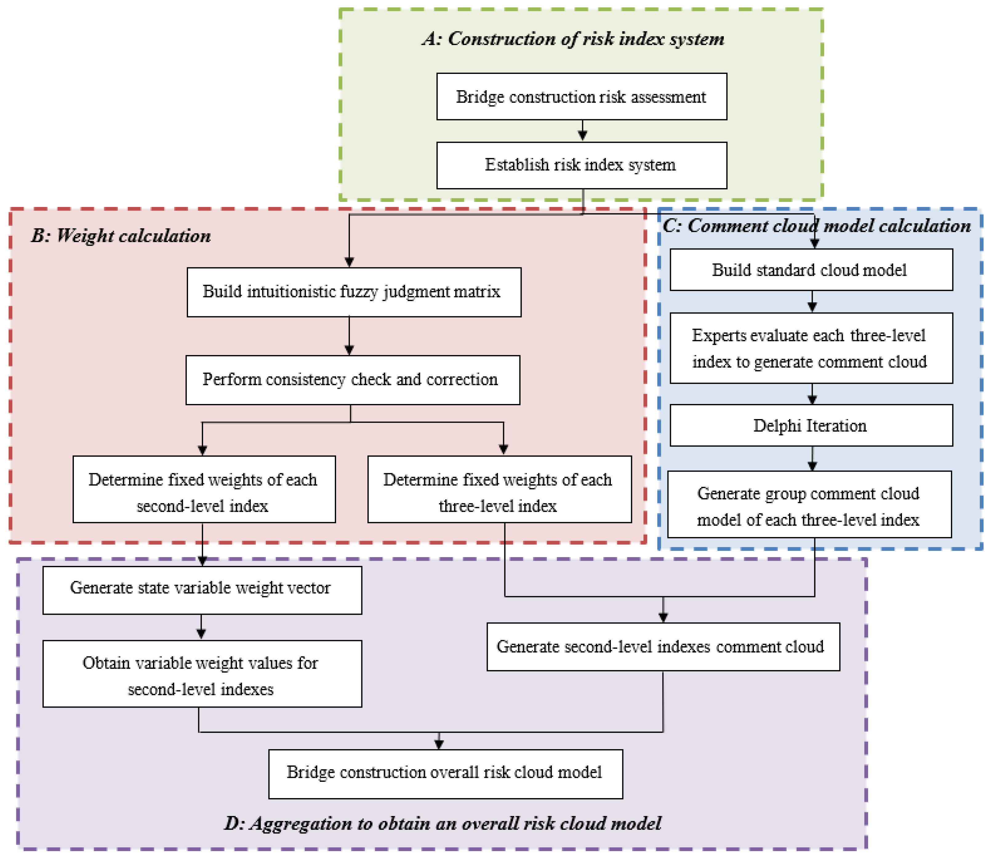
3. Bridge Construction Risk Assessment Model
3.1. Establish Risk Index System
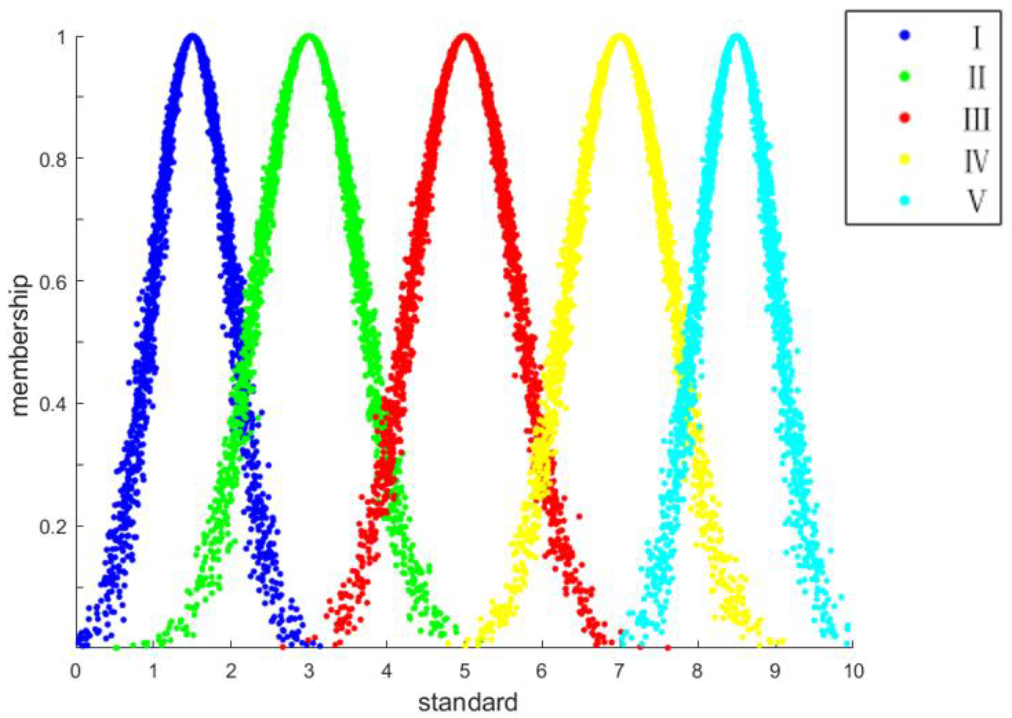
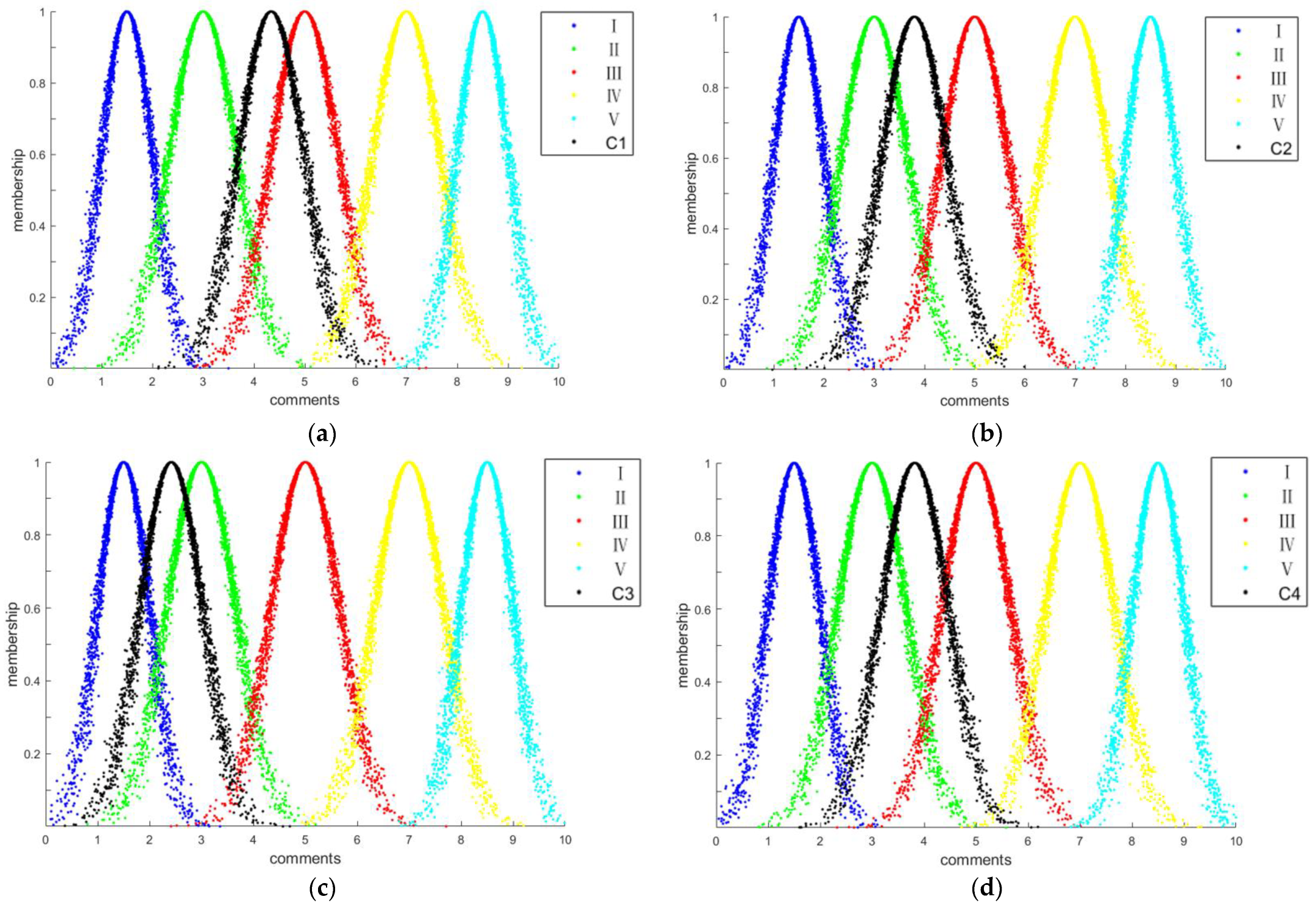
3.2. Build Standard Cloud Model
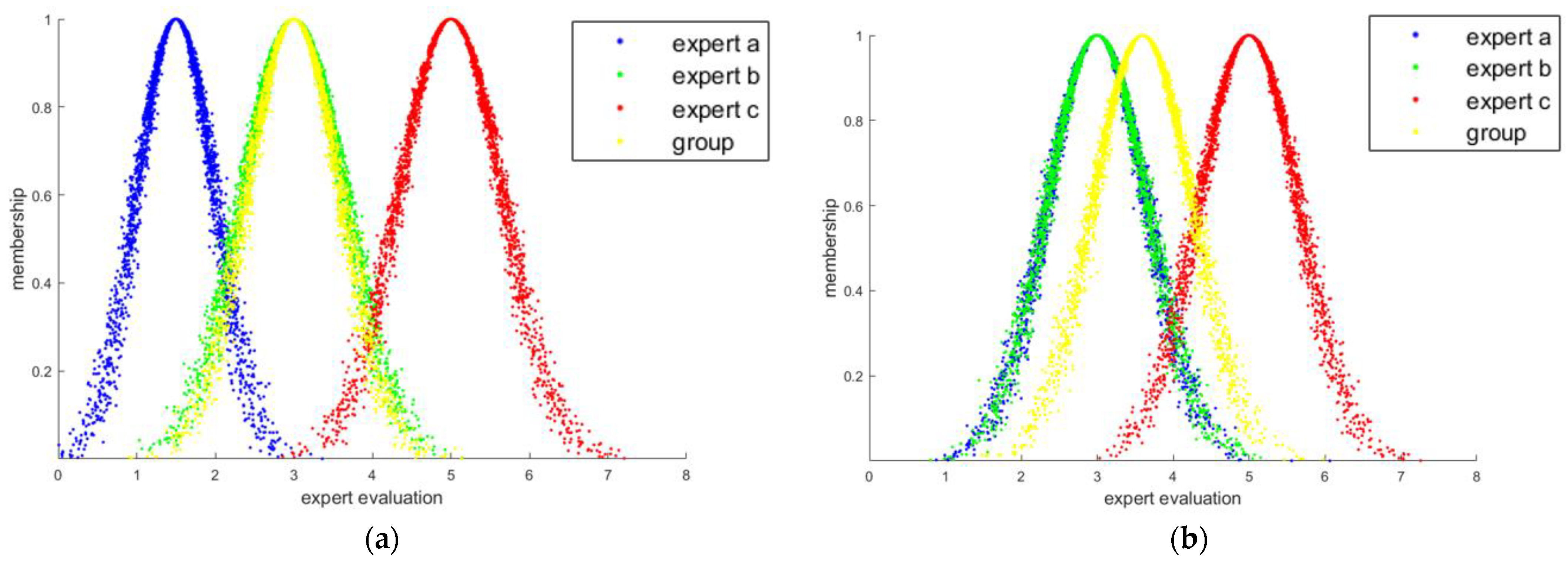
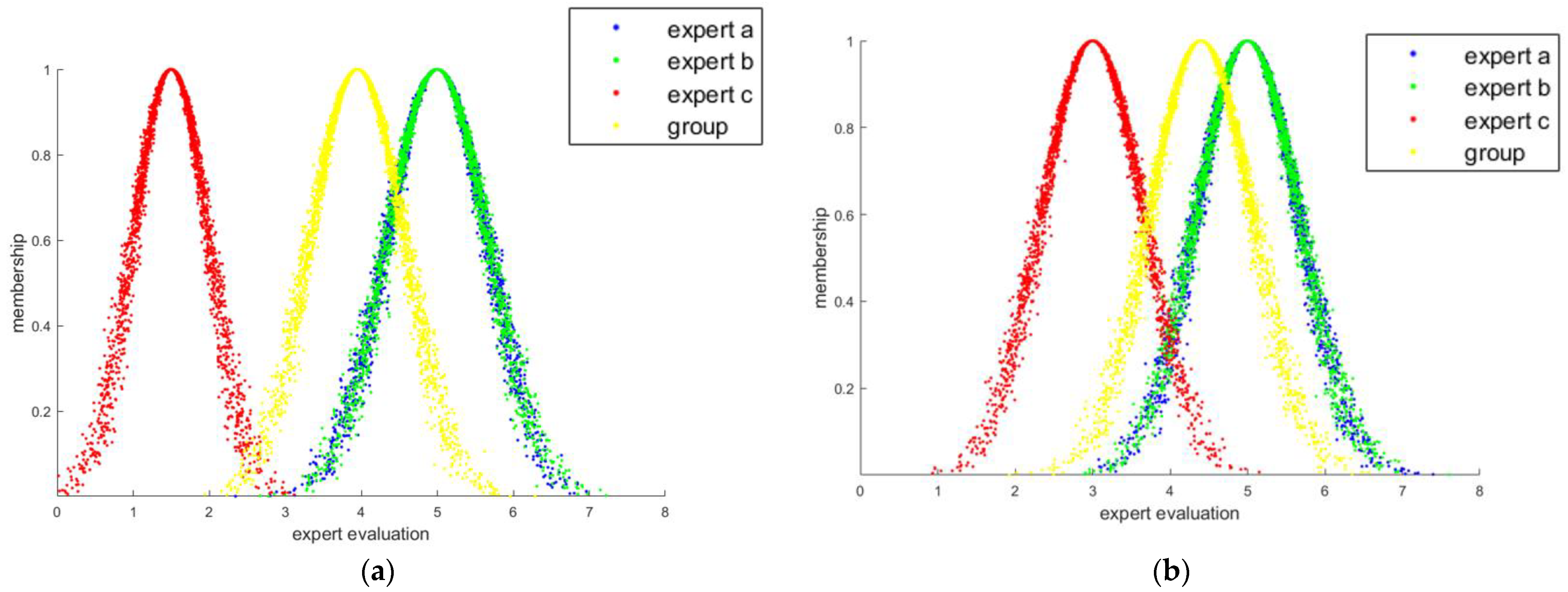
3.3. Build Comment Cloud Model
3.4. Calculate the Fixed Weight of Indexes
- (1)
- If , .
- (2)
- If or , .
- (3)
- If , .
3.5. Calculate the Variable Weight of Indexes
4. Project Case
4.1. Project Overview
4.2. Calculate Three-Level Indexes Comment Cloud Model
4.3. Calculate Indexes Weight
4.3.1. Fixed Weight Calculation of Three-Level Indexes Based on IFAHP
4.3.2. Variable Weight Calculation of Second-Level Indexes Based on Variable Weight Theory
4.4. Aggregate to Obtain the Risk Level
5. Comparison and Discussion
5.1. Accuracy Verification
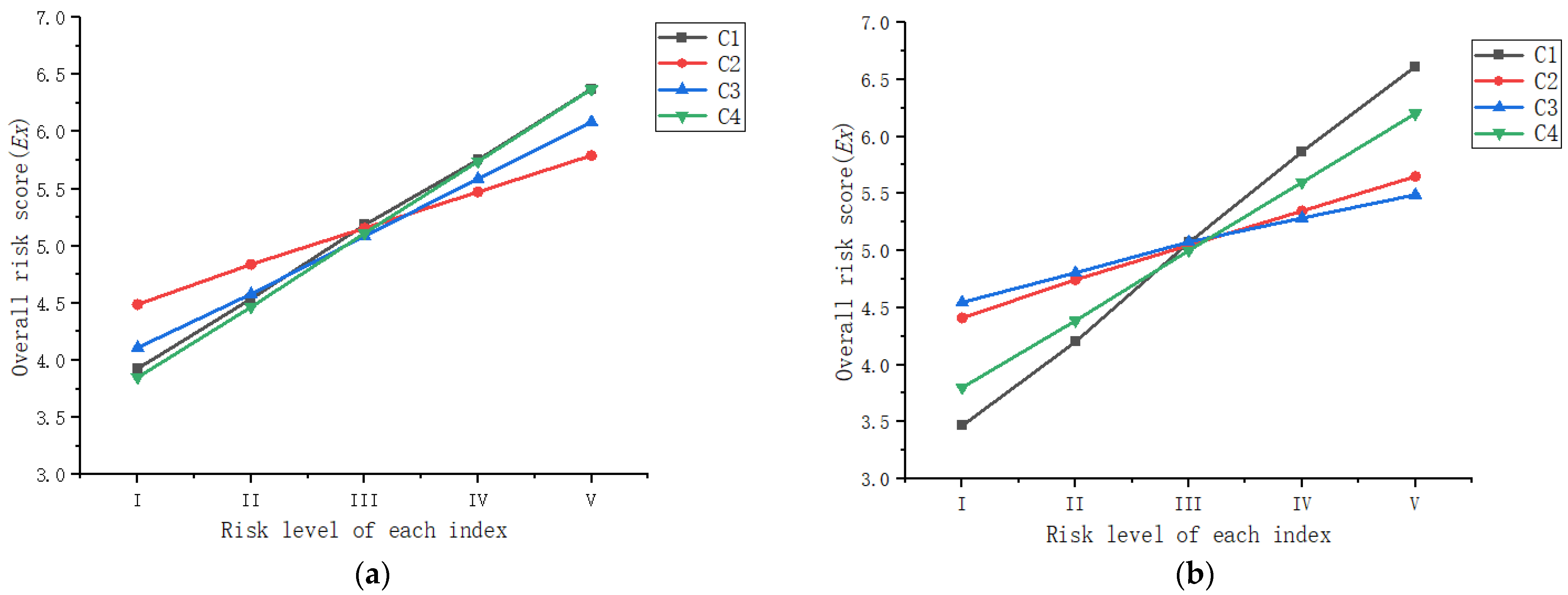
5.2. Sensitivity Analysis
6. Conclusions
- (1)
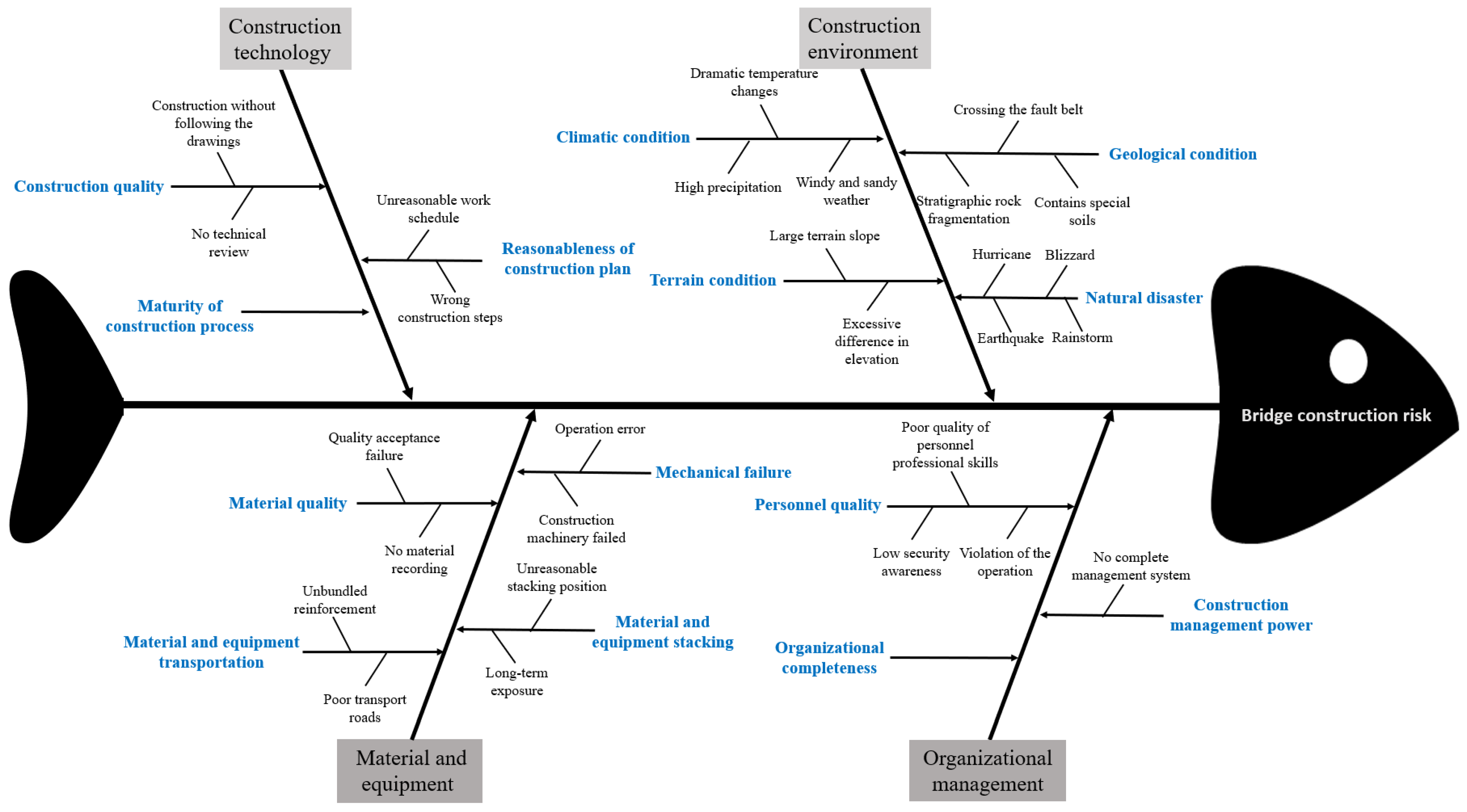
- In this paper, the fishbone diagram analysis method was adopted to analyze the causes of construction risks, and 14 risk factors that affect bridge construction safety were identified. A risk index system with a three-level structure was constructed, and the accuracy of the evaluation results was ensured through step-by-step calculations.
- (2)
- In this paper, the cloud model was used to construct the evaluation model to express the fuzziness and randomness of the expert comments. At the same time, the cloud model was used throughout the evaluation process, expressing the uncertainty of the evaluation process effectively. The Delphi iterative method was used to eliminate the subjective bias of individual experts to a greater extent. IFAHP was used to calculate index weights to solve the hesitancy arising from the experts’ decision-making process, ensuring the integrity of the expert’s opinions in the assessment model. With the variable weight theory applied and the zoning variable weight function constructed, the weight distribution of the second-level index construction risk is optimized by “penalty” and “incentive” to the index weights.
- (3)
- In this paper, a whole bridge construction risk assessment system is constructed and applied to the actual project of a bridge in Changchun. The advancement of the assessment system in this paper is well verified by the results analysis of the intermediate process of the example calculation. Finally, accuracy verification and sensitivity analysis are conducted to verify the validity and feasibility of the assessment system.
Author Contributions
Funding
Data Availability Statement
Conflicts of Interest
References
- Mortazavi, S.; Kheyroddin, A.; Naderpour, H. Risk Evaluation and Prioritization in Bridge Construction Projects Using System Dynamics Approach. Pract. Period. Struct. Des. Constr. 2020, 25, 04020015. [Google Scholar] [CrossRef]
- Nieto-Morote, A.; Ruz-Vila, F. A Fuzzy Approach to Construction Project Risk Assessment. Int. J. Proj. Manag. 2011, 29, 220–231. [Google Scholar] [CrossRef]
- Andric, J.M.; Lu, D.-G. Risk Assessment of Bridges under Multiple Hazards in Operation Period. Saf. Sci. 2016, 83, 80–92. [Google Scholar] [CrossRef]
- Kim, J.-M.; Kim, T.; Ahn, S. Loss Assessment for Sustainable Industrial Infrastructure: Focusing on Bridge Construction and Financial Losses. Sustainability 2020, 12, 5316. [Google Scholar] [CrossRef]
- Wang, M.; Niu, D. Research on Project Post-Evaluation of Wind Power Based on Improved ANP and Fuzzy Comprehensive Evaluation Model of Trapezoid Subordinate Function Improved by Interval Number. Renew. Energy 2019, 132, 255–265. [Google Scholar] [CrossRef]
- Peng, K. Risk Evaluation for Bridge Engineering Based on Cloud-Clustering Group Decision Method. J. Perform. Constr. Facil. 2019, 33, 04018105. [Google Scholar] [CrossRef]
- Liang, X.; Liang, W.; Zhang, L.; Guo, X. Risk Assessment for Long-Distance Gas Pipelines in Coal Mine Gobs Based on Structure Entropy Weight Method and Multi-Step Backward Cloud Transformation Algorithm Based on Sampling with Replacement. J. Clean Prod. 2019, 227, 218–228. [Google Scholar] [CrossRef]
- Li, X.; Chen, G.; Zhu, H. Quantitative Risk Analysis on Leakage Failure of Submarine Oil and Gas Pipelines Using Bayesian Network. Process Saf. Environ. Prot. 2016, 103, 163–173. [Google Scholar] [CrossRef]
- Li, Q.; Zhou, J.; Feng, J. Safety Risk Assessment of Highway Bridge Construction Based on Cloud Entropy Power Method. Appl. Sci. 2022, 12, 8692. [Google Scholar] [CrossRef]
- Ji, T.; Liu, J.-W.; Li, Q.-F. Safety Risk Evaluation of Large and Complex Bridges during Construction Based on the Delphi-Improved FAHP-Factor Analysis Method. Adv. Civ. Eng. 2022, 2022, e5397032. [Google Scholar] [CrossRef]
- He, K.; Zhu, J.; Wang, H.; Huang, Y.; Li, H.; Dai, Z.; Zhang, J. Safety Risk Evaluation of Metro Shield Construction When Undercrossing a Bridge. Buildings 2023, 13, 2540. [Google Scholar] [CrossRef]
- Dawood, T.; Elwakil, E.; Mayol Novoa, H.; Garate Delgado, J.F. Soft Computing for Modeling Pipeline Risk Index under Uncertainty. Eng. Fail. Anal. 2020, 117, 104949. [Google Scholar] [CrossRef]
- Wang, X.; Li, S.; Xu, Z.; Li, X.; Lin, P.; Lin, C. An Interval Risk Assessment Method and Management of Water Inflow and Inrush in Course of Karst Tunnel Excavation. Tunn. Undergr. Space Technol. 2019, 92, 103033. [Google Scholar] [CrossRef]
- Badida, P.; Balasubramaniam, Y.; Jayaprakash, J. Risk Evaluation of Oil and Natural Gas Pipelines Due to Natural Hazards Using Fuzzy Fault Tree Analysis. J. Nat. Gas Sci. Eng. 2019, 66, 284–292. [Google Scholar] [CrossRef]
- Huang, Z.; Zhang, W.; Sun, H.; Pan, Q.; Zhang, J.; Li, Y. Risk Uncertainty Analysis in Shield Tunnel Projects. Tunn. Undergr. Space Technol. 2023, 132, 104899. [Google Scholar] [CrossRef]
- Li, X.; Yang, M.; Chen, G. An Integrated Framework for Subsea Pipelines Safety Analysis Considering Causation Dependencies. Ocean Eng. 2019, 183, 175–186. [Google Scholar] [CrossRef]
- Wang, L.; Jin, R.; Zhou, J.; Li, Q. Construction Risk Assessment of Yellow River Bridges Based on Combined Empowerment Method and Two-Dimensional Cloud Model. Appl. Sci. 2023, 13, 10942. [Google Scholar] [CrossRef]
- Li, H.X.; Li, L.X.; Wang, J.Y.; Mo, Z.; Li, Y.D. Fuzzy Decision Making Based on Variable Weights. Math. Comput. Model. 2004, 39, 163–179. [Google Scholar] [CrossRef]
- Lin, C.; Zhang, M.; Zhou, Z.; Li, L.; Shi, S.; Chen, Y.; Dai, W. A New Quantitative Method for Risk Assessment of Water Inrush in Karst Tunnels Based on Variable Weight Function and Improved Cloud Model. Tunn. Undergr. Space Technol. 2020, 95, 103136. [Google Scholar] [CrossRef]
- Li, D.; Liu, C.; Gan, W. A New Cognitive Model: Cloud Model. Int. J. Intell. Syst. 2009, 24, 357–375. [Google Scholar] [CrossRef]
- Chen, Y.; Xie, S.; Tian, Z. Risk Assessment of Buried Gas Pipelines Based on Improved Cloud-Variable Weight Theory. Reliab. Eng. Syst. Saf. 2022, 221, 108374. [Google Scholar] [CrossRef]
- Xu, Z.; Liao, H. Intuitionistic Fuzzy Analytic Hierarchy Process. IEEE Trans. Fuzzy Syst. 2014, 22, 749–761. [Google Scholar] [CrossRef]
- Atanassov, K. Intuitionistic Fuzzy Sets; Springer: New York, NY, USA, 1999. [Google Scholar]
- Wang, Y.; Xu, Z. Evaluation of the Human Settlement in Lhasa with Intuitionistic Fuzzy Analytic Hierarchy Process. Int. J. Fuzzy Syst. 2018, 20, 29–44. [Google Scholar] [CrossRef]
- Wang, X.; Li, S.; Xu, Z.; Hu, J.; Pan, D.; Xue, Y. Risk Assessment of Water Inrush in Karst Tunnels Excavation Based on Normal Cloud Model. Bull. Eng. Geol. Environ. 2019, 78, 3783–3798. [Google Scholar] [CrossRef]
- Liu, H.; Wang, L.; Li, Z.; Hu, Y. Improving Risk Evaluation in FMEA With Cloud Model and Hierarchical TOPSIS Method. IEEE Trans. Fuzzy Syst. 2019, 27, 84–95. [Google Scholar] [CrossRef]
- Wu, Y.; Chu, H.; Xu, C. Risk Assessment of Wind-Photovoltaic-Hydrogen Storage Projects Using an Improved Fuzzy Synthetic Evaluation Approach Based on Cloud Model: A Case Study in China. J. Energy Storage 2021, 38, 102580. [Google Scholar] [CrossRef]
- Xu, Z. Intuitionistic Preference Relations and Their Application in Group Decision Making. Inf. Sci. 2007, 177, 2363–2379. [Google Scholar] [CrossRef]
- Li, X.; Zhang, W.; Wang, X.; Wang, Z.; Pang, C. Evaluation on the Risk of Water Inrush Due to Roof Bed Separation Based on Improved Set Pair Analysis−Variable Fuzzy Sets. ACS Omega 2022, 7, 9430–9442. [Google Scholar] [CrossRef] [PubMed]
- Yu, X.; Liang, W.; Zhang, L.; Reniers, G.; Lu, L. Risk Assessment of the Maintenance Process for Onshore Oil and Gas Transmission Pipelines under Uncertainty. Reliab. Eng. Syst. Saf. 2018, 177, 50–67. [Google Scholar] [CrossRef]


| Literature | Risk Analysis Methods | Uncertainty Expression Methods | Weight Determination Methods |
|---|---|---|---|
| Liang et al. [7] | Fault Tree Analysis (FTA) | Cloud model (CM) | Entropy weight method |
| Dawood et al. [12] | Risk index system | Fuzzy set theory | - |
| Wang and Niu [5] | Risk index system | Fuzzy set theory | ANP |
| Wang et al. [13] | Risk index system | Fuzzy set theory | AHP |
| Badida et al. [14] | Fault Tree Analysis (FTA) | Fuzzy set theory | - |
| Huang et al. [15] | Risk index system | Cloud model (CM) | AHP |
| Li et al. [16] | Risk index system | - | Decision-making trial and Evaluation |
| Wang et al. [17] | Risk index system | Cloud model (CM) | AHP, Entropy weight method |
| Risk Level | Risk Description | Score Range | Digital Features |
|---|---|---|---|
| I | Very low risk | (0–2) | (1.5, 0.5, 0.05) |
| II | Low risk | (2–4) | (3, 0.66, 0.05) |
| III | Medium risk | (4–6) | (5, 0.66, 0.05) |
| IV | High risk | (6–8) | (7, 0.66, 0.05) |
| V | Very high risk | (8–10) | (8.5, 0.5, 0.05) |
| Aspects | Classification | Score |
|---|---|---|
| Work experience | Under 5 years | 1 |
| 5–14 years | 2 | |
| 15–19 years | 3 | |
| Over 20 years | 4 | |
| Positional title | Junior | 2 |
| Intermediate | 3 | |
| Senior | 4 |
| Scale | Relative Relationship of Indexes |
|---|---|
| 0.9 | Index i is absolutely more important than j |
| 0.8 | Index i is largely more important than j |
| 0.7 | Index i is essentially more important than j |
| 0.6 | Index i is slightly more important than j |
| 0.5 | Index i is as important as j |
| 0.4 | Index j is slightly more important than i |
| 0.3 | Index j is essentially more important than i |
| 0.2 | Index j is largely more important than i |
| 0.1 | Index j is absolutely more important than i |
| Experts | C11 | C12 | C13 | C14 |
|---|---|---|---|---|
| Expert a | I (1.5, 0.5, 0.05) | III (5, 0.66, 0.05) | IV (7, 0.66, 0.05) | I (5, 0.66, 0.05) |
| Expert b | II (3, 0.66, 0.05) | III (5, 0.66, 0.05) | IV (7, 0.66, 0.05) | II (3, 0.66, 0.05) |
| Expert c | III (5, 0.66, 0.05) | I (1.5, 0.5, 0.05) | III (7, 0.66, 0.05) | I (3, 0.66, 0.05) |
| Group | (3, 0.60, 0.05) | (3.95, 0.66, 0.05) | (7, 0.66, 0.05) | (3.8, 0.66, 0.05) |
| Experts | C11 | C12 | C13 | C14 |
|---|---|---|---|---|
| Expert a | II (3, 0.66, 0.05) | III (5, 0.66, 0.05) | IV (7, 0.66, 0.05) | I (5, 0.66, 0.05) |
| Expert b | II (3, 0.66, 0.05) | III (5, 0.66, 0.05) | IV (7, 0.66, 0.05) | II (3, 0.66, 0.05) |
| Expert c | III (5, 0.66, 0.05) | II (3, 0.66, 0.05) | III (7, 0.66, 0.05) | I (3, 0.66, 0.05) |
| Group | (3.6, 0.66, 0.05) | (4.4, 0.66, 0.05) | (7, 0.66, 0.05) | (3.8, 0.66, 0.05) |
| Three-Level Indexes | Group Comment Cloud Model |
|---|---|
| C11 | (3.6, 0.66, 0.05) |
| C12 | (4.4, 0.66, 0.05) |
| C13 | (7, 0.66, 0.05) |
| C14 | (3.8, 0.66, 0.05) |
| C21 | (2.55, 0.62, 0.05) |
| C22 | (3.8, 0.66, 0.05) |
| C23 | (4.4, 0.66, 0.05) |
| C31 | (2.55, 0.62, 0.05) |
| C32 | (3, 0.66, 0.05) |
| C33 | (1.95, 0.55, 0.05) |
| C34 | (2.4, 0.6, 0.05) |
| C41 | (3, 0.66, 0.05) |
| C42 | (2.55, 0.62, 0.05) |
| C43 | (5.6, 0.66, 0.05) |
| Three-Level Indexes | Fixed Weight |
|---|---|
| C11 | 0.203 |
| C12 | 0.317 |
| C13 | 0.288 |
| C14 | 0.192 |
| C21 | 0.219 |
| C22 | 0.318 |
| C23 | 0.463 |
| C31 | 0.186 |
| C32 | 0.226 |
| C33 | 0.324 |
| C34 | 0.264 |
| C41 | 0.396 |
| C42 | 0.247 |
| C43 | 0.357 |
| Second-Level Indexes | Fixed Weight | Variable Weight |
|---|---|---|
| C1 | 0.297 | 0.310 |
| C2 | 0.158 | 0.150 |
| C3 | 0.251 | 0.239 |
| C4 | 0.316 | 0.301 |
| Second-Level Indexes | Comment Cloud Model | Risk Level |
|---|---|---|
| C1 | (4.87, 0.66, 0.05) | III |
| C2 | (3.80, 0.65, 0.05) | II |
| C3 | (2.42, 0.60, 0.05) | II |
| C4 | (3.82, 0.65, 0.05) | II |
| Indexes | This Paper’s Method | Fuzzy Comprehensive Evaluation Method |
|---|---|---|
| C1 | III (4.87, 0.66, 0.05) | III (4.25) |
| C2 | II (3.80, 0.65, 0.05) | II (3.25) |
| C3 | II (2.42, 0.60, 0.05) | II (2.87) |
| C4 | II (3.82, 0.65, 0.05) | II (3.67) |
| Evaluation Target | This Paper’s Method | Fuzzy Comprehensive Evaluation Method |
|---|---|---|
| Overall risk cloud model | (3.81, 0.64, 0.05) | 3.59 |
| Risk level | II (low risk) | II (low risk) |
| Case | Location | Project Overview |
|---|---|---|
| 1 | Zhejiang | The proposed bridge is a prestressed concrete continuous box-girder bridge with a span arrangement of (25 × 30) m. The average annual temperature at the bridge site is 16.3 °C, and the climate is mild and humid. The stratigraphic distribution at the bridge site is silty clay and limestone. The bridge site belongs to the low mountains and hills area with a difference of 30 m in elevation. |
| 2 | Liaoning | The proposed bridge is a prestressed concrete box girder with a span arrangement of (55 + 80 + 5 × 30) m. The bridge site has cold winters and warm summers with four distinct seasons, and the average annual temperature is 8.5 °C. The bridge crosses an asymmetrical V-shaped valley with a relative height difference of up to 50 m. The stratigraphic distribution is mainly silty clay and limestone. |
| 3 | Hubei | The proposed bridge is an assembled prestressed concrete continuous box-girder bridge with a span arrangement of (11 × 30) m. The bridge site is hot in summer and cold in winter, humid and rainy, with an average annual temperature of 16.7 °C. The bridge site belongs to the hilly and plain area with little topographic relief. The stratigraphic distribution is mainly clay soil, fine sand, gravel, shaly sandstone, and sandy mudstone. |
| 4 | Henan | The proposed bridge is an assembled prestressed concrete continuous T-beam bridge with a span arrangement of (6 × 50) m. The climate at the bridge site is warm with four distinct seasons and an average annual temperature of 14.2 °C. The bridge site area belongs to hilly topography with large relief, and the ground elevation is around 352.5–386.4. Within the exploration depth, the stratigraphic distribution is mainly loess, clay, and gravel. |
| 5 | Henan | The proposed bridge is an assembled prestressed concrete continuous box-girder bridge with a span arrangement of (4 × 20 + 5 × 20) m. The bridge site has a temperate continental monsoon climate with four distinct seasons and an average annual temperature of 12.9 °C. The bridge area is in the mountainous area of the eastern extension of the Qinling Mountains with obvious terrain changes. The stratigraphic distribution is mainly backfilling soil, sandy loess, gravelly soil, and sand conglomerate. The main special geotechnical soil in the bridge site area is sandy loess, which is middle collapsible loess with a collapse coefficient of 0.048. |
| 6 | Henan | The proposed bridge is a continuous rigid frame bridge with a span arrangement of (4 × 40 + 85 + 5 × 40) m. The bridge site has a temperate continental monsoon climate with low precipitation and an average annual temperature of 13.8 °C. The bridge site is mainly farmland, and the terrain is relatively flat. The stratigraphic distribution is mainly backfilling soil, silty clay, fine sand, and pebbles. |
| 7 | Jiangsu | The total length of the proposed bridge is 420 m, and the bridge site area belongs to the subtropical humid climate zone with the average annual temperature ranging from 13 to 16 °C. The proposed site belongs to the shallow plain area, and the stratigraphic structure mainly consists of clay and silt layers. |
| Case | Samples Name | This Paper’s Method | Fuzzy Comprehensive Evaluation Method |
|---|---|---|---|
| 1 | Zhejiang | II (2.54, 0.64, 0.05) | II (2.67) |
| 2 | Liaoning | II (3.62, 0.63, 0.05) | II (3.44) |
| 3 | Hubei | I (1.78, 0.62, 0.05) | I (1.93) |
| 4 | Henan 1 | II (3.18, 0.59, 0.05) | II (3.23) |
| 5 | Henan 2 | III (4.36, 0.63, 0.05) | III (4.10) |
| 6 | Henan 3 | I (1.14, 0.57, 0.05) | I (1.53) |
| 7 | Jiangsu | I (2.06, 0.66, 0.05) | I (2.13) |
| Second-Level Indexes | Sensitivity under Fixed Weights | Sensitivity under Variable Weights |
|---|---|---|
| C1 | 0.6114 | 0.7864 |
| C2 | 0.3257 | 0.3401 |
| C3 | 0.4940 | 0.2354 |
| C4 | 0.6301 | 0.6002 |
Disclaimer/Publisher’s Note: The statements, opinions and data contained in all publications are solely those of the individual author(s) and contributor(s) and not of MDPI and/or the editor(s). MDPI and/or the editor(s) disclaim responsibility for any injury to people or property resulting from any ideas, methods, instructions or products referred to in the content. |
© 2024 by the authors. Licensee MDPI, Basel, Switzerland. This article is an open access article distributed under the terms and conditions of the Creative Commons Attribution (CC BY) license (https://creativecommons.org/licenses/by/4.0/).
Share and Cite
Yao, B.; Wang, L.; Gao, H.; Ren, L. Bridge Construction Risk Assessment Based on Variable Weight Theory and Cloud Model. Buildings 2024, 14, 576. https://doi.org/10.3390/buildings14030576
Yao B, Wang L, Gao H, Ren L. Bridge Construction Risk Assessment Based on Variable Weight Theory and Cloud Model. Buildings. 2024; 14(3):576. https://doi.org/10.3390/buildings14030576
Chicago/Turabian StyleYao, Bo, Lianguang Wang, Haiyang Gao, and Lijie Ren. 2024. "Bridge Construction Risk Assessment Based on Variable Weight Theory and Cloud Model" Buildings 14, no. 3: 576. https://doi.org/10.3390/buildings14030576