
Prediction of the Unconfined Compressive Strength of Salinized Frozen Soil Based on Machine Learning

Abstract
:1. Introduction
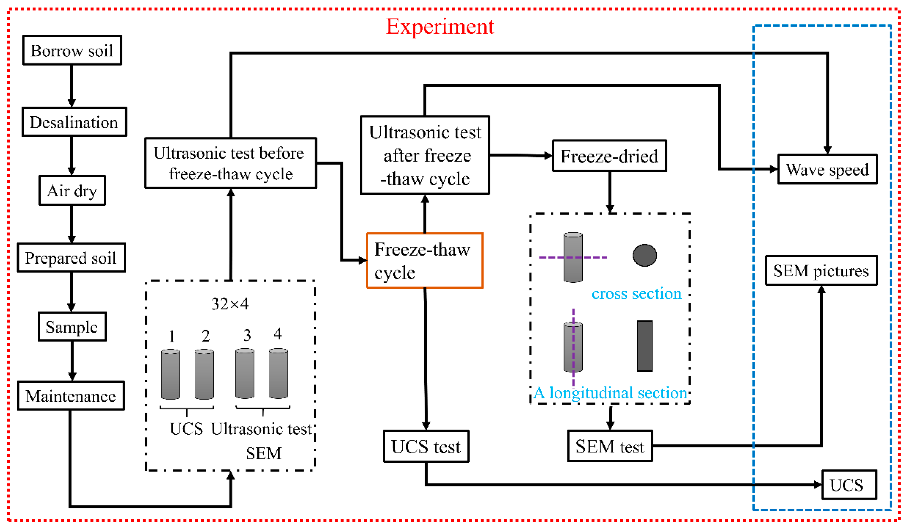
2. Experiment
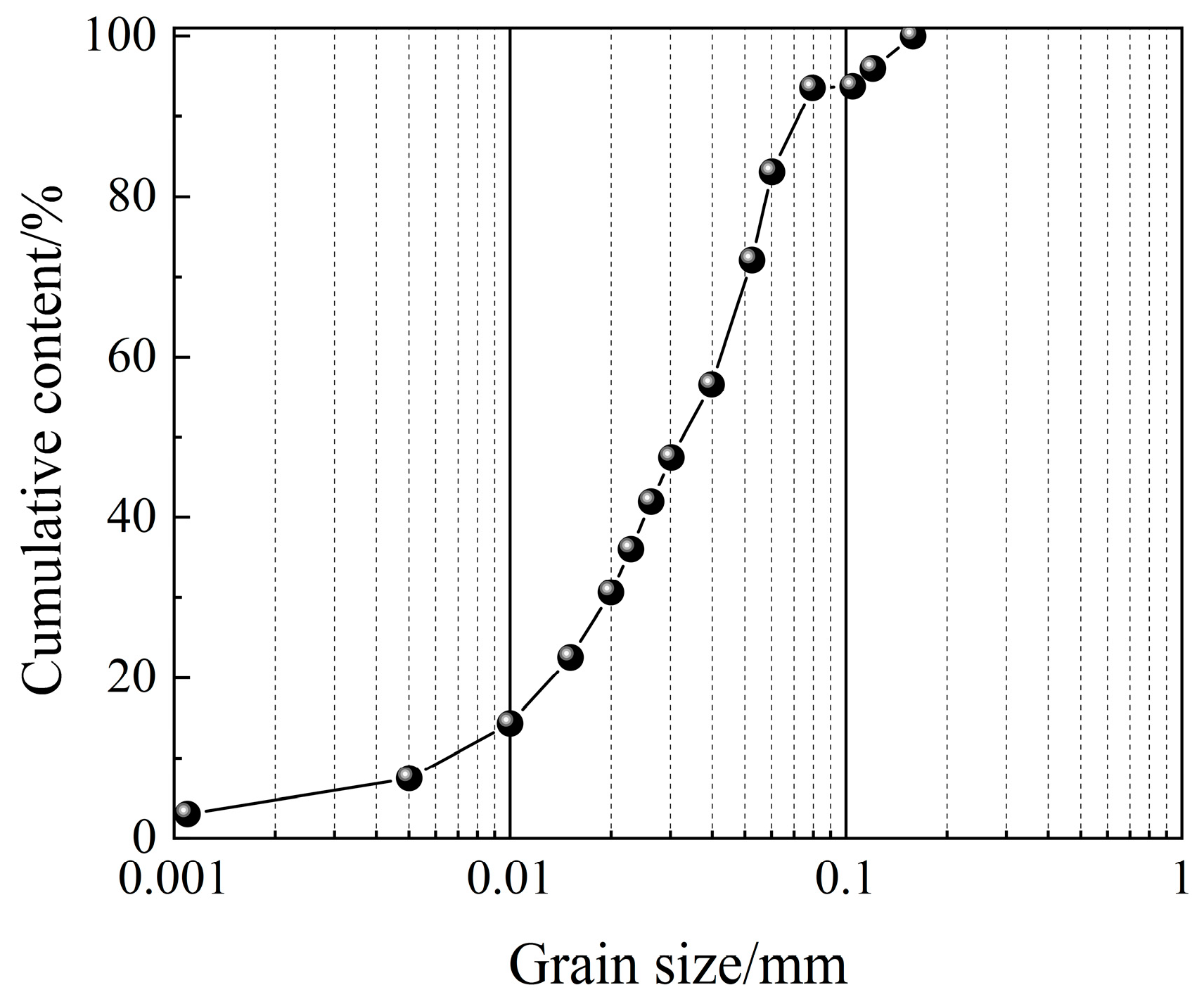
2.1. Basic Physical Properties of Soil Samples and Sample Preparation
2.2. Test Methods and Procedures
2.2.1. UCS Test
- (1)
- Remove the plastic wrap of the sample, polish the surface to ensure smoothness, and then start the UCS test.
- (2)
- After the test is completed, the stress–strain data corresponding to the .gds format is automatically output. Subsequently, through Origin drawing, the peak stress of the curve is selected as the UCS value of the sample.
2.2.2. Ultrasonic Testing
- (1)
- Add a sample with the upper and lower bottom surfaces brushed with Vaseline as coupling agent. Note that the lower bottom surface of the sample is close to the receiving transducer, and the upper bottom surface is close to the pressure-bearing transmitting transducer. After the sample loading is completed, the wave speed test begins.
- (2)
- Each test item is drawn and recorded three times as waveform data by the acoustic wave detector. After the collection is completed, .SHT and .SHD format files are output. Subsequently, with the help of the oscilloscope software corresponding (RSM acoustic intensity analysis software, V1.1.220310) to the detector and the initial arrival wave method [45,46], the wave propagation time and the sample acoustic wave speed are obtained.
2.2.3. SEM Test
- (1)
- Freeze-dry the sample and obtain a fresh cross-section cube of about 8 mm by cutting near the middle part of the sample along the direction perpendicular to the Z-axis as a cross-section sample (The Z-axis is parallel to the height direction of the sample). Cut along the direction perpendicular to the X and Y axes to obtain a fresh cross-section cube of about 8 mm as a longitudinal cross-section sample. The sample to be tested is then fixed on the metal stage, coated, and sent to the sample chamber.
- (2)
- Start the test program and enter relevant test parameters. Focus at high magnification first, and then look for a suitable area under low magnification conditions. After selecting the test area, the position will no longer move, and 500X, 1000X, and 2000X shooting will be performed in sequence.
2.3. Analysis of Test Results
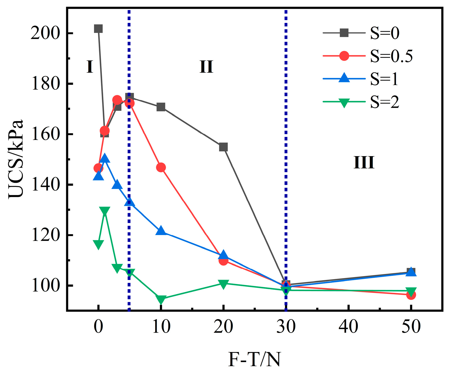
2.3.1. The Impact of Control Factors on UCS
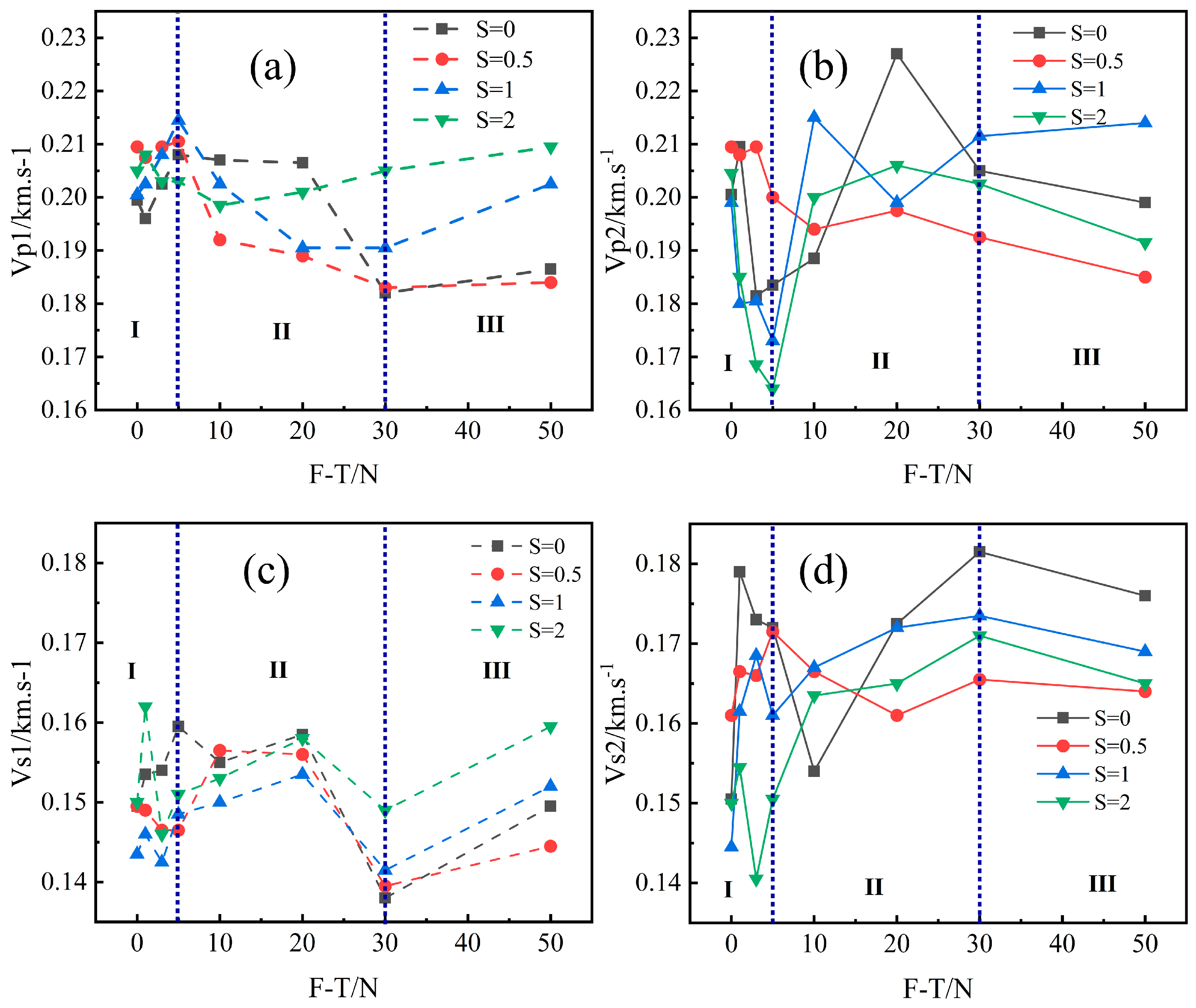
2.3.2. Influence of Control Factors on Wave Speed
2.3.3. The Influence of Control Factors on SEM Characteristic Parameters
- (1)
- Probability entropy
- (2)
- Probability distribution index
- (3)
- Fractal dimension
- (4)
- Porosity
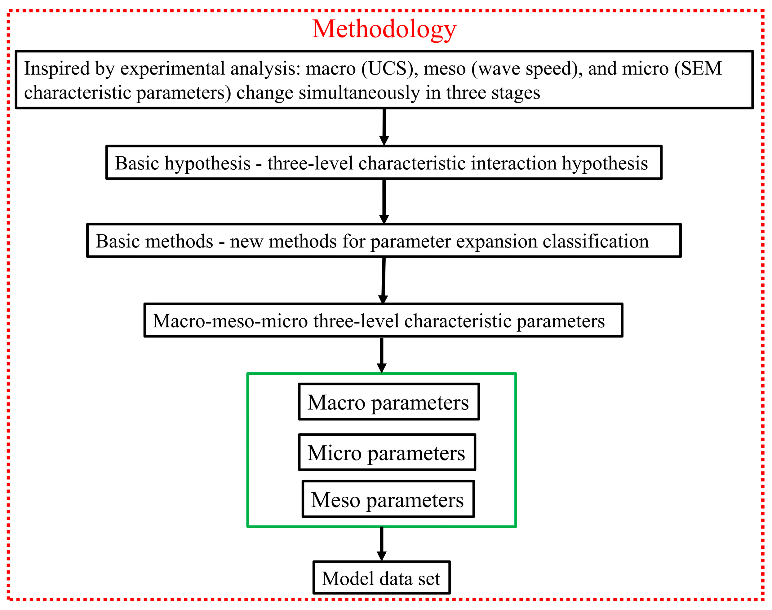
3. Methodology
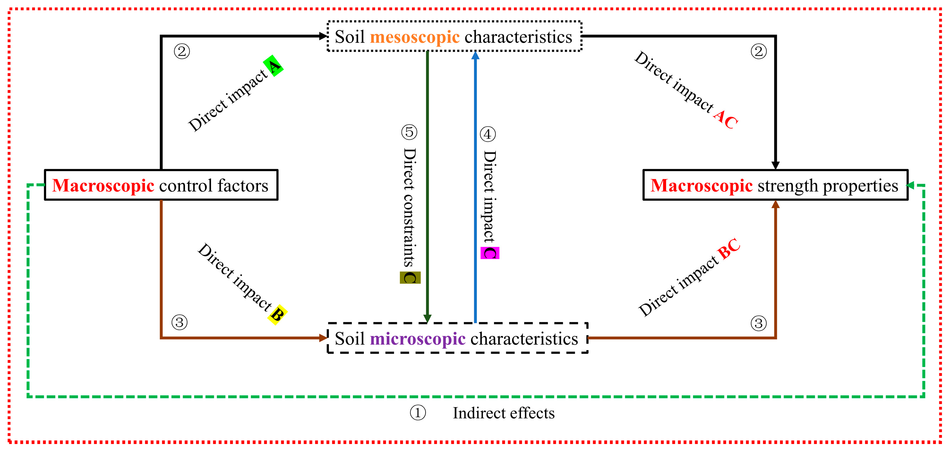
3.1. Basic Hypothesis-Three-Level Characteristic Interaction Hypothesis
3.2. Basic Methods-New Methods for Parameter Expansion Classification
3.3. Macro–Meso–Micro Three-Level Characteristic Parameters
3.3.1. Macro Parameters
3.3.2. Meso Parameters
3.3.3. Micro Parameters
3.4. Model Data Set
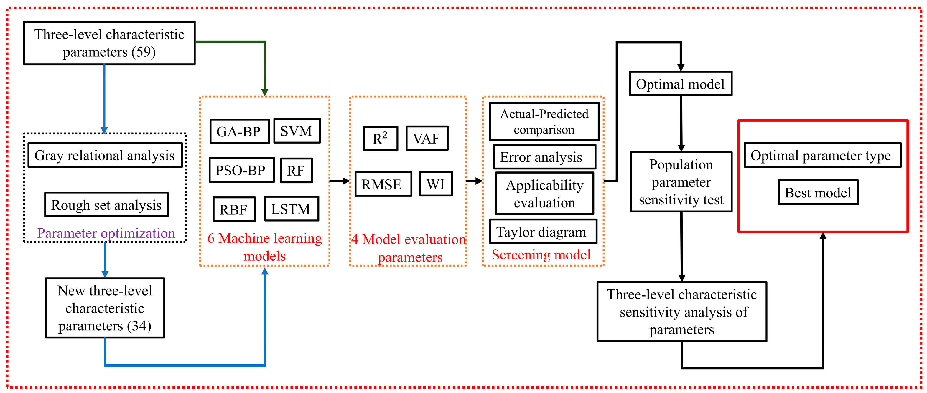
4. Methodology Applied to the Model
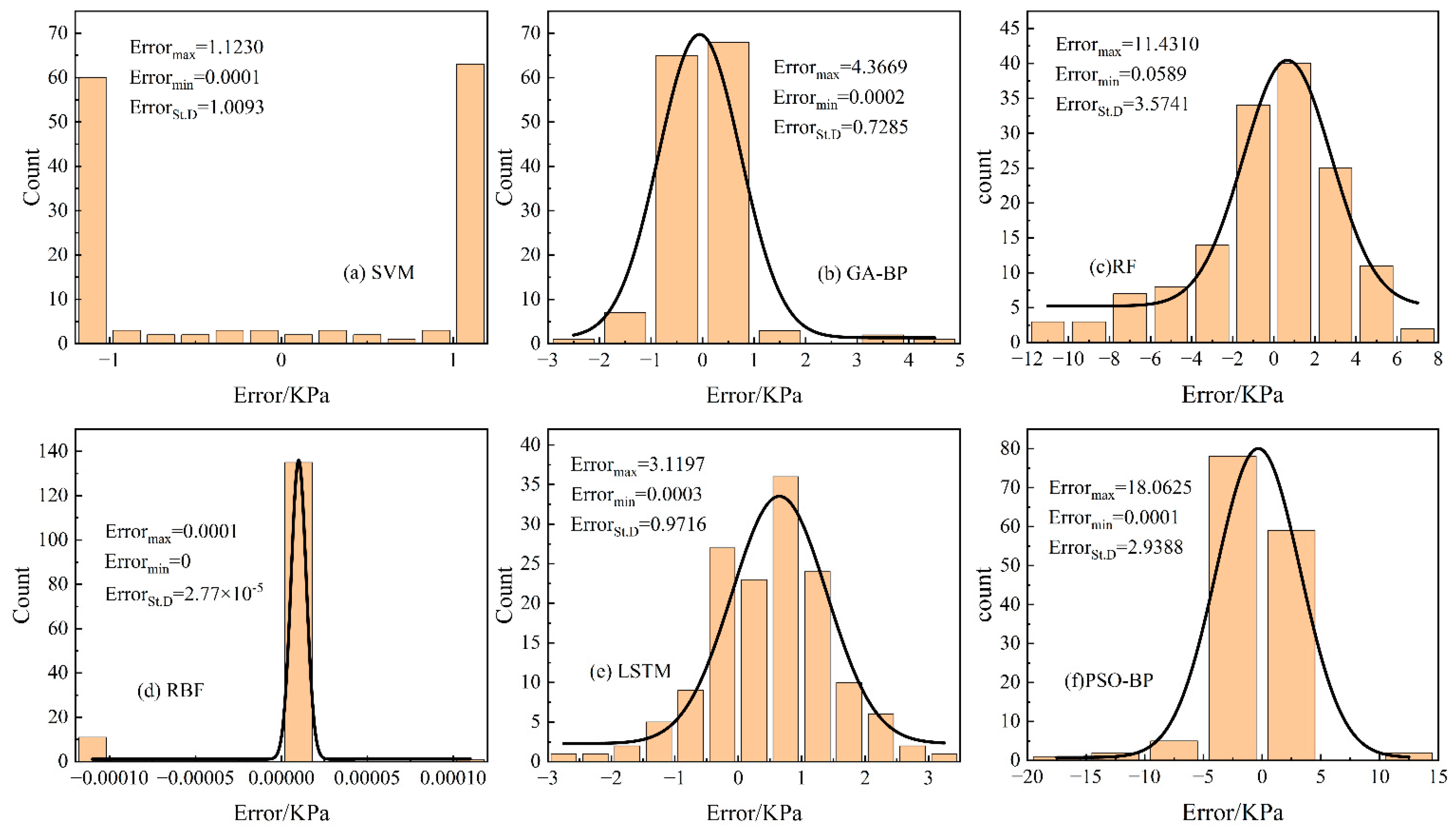
4.1. 6 Machine Learning Models
- (1)
- Support vector machine (SVM)
- (2)
- Genetic algorithm optimized BP (GA-BP)
- (3)
- Random forest (RF)
- (4)
- Radial basis function (RBF)
- (5)
- Long short-term memory (LSTM)
- (6)
- Particle swarm optimization algorithm BP (PSO-BP)
4.2. Evaluation Indicators
4.3. Model Analysis and Hyperparameters
5. Results and Discussion
5.1. Model Prediction of the 59 Total Parameters
5.1.1. 59-Parameter Optimal Model
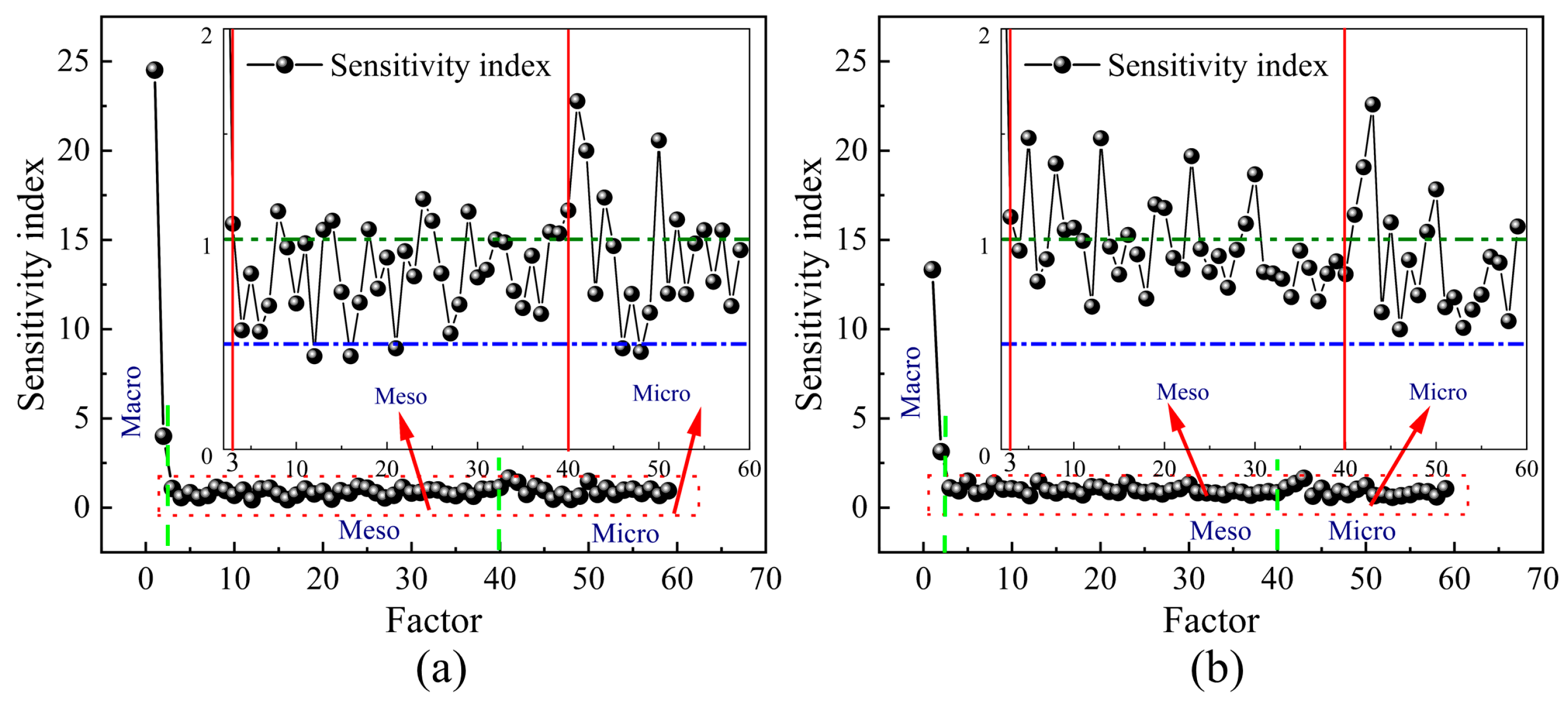
5.1.2. Single Parameter Sensitivity Test of 59-Parameter Optimal Model
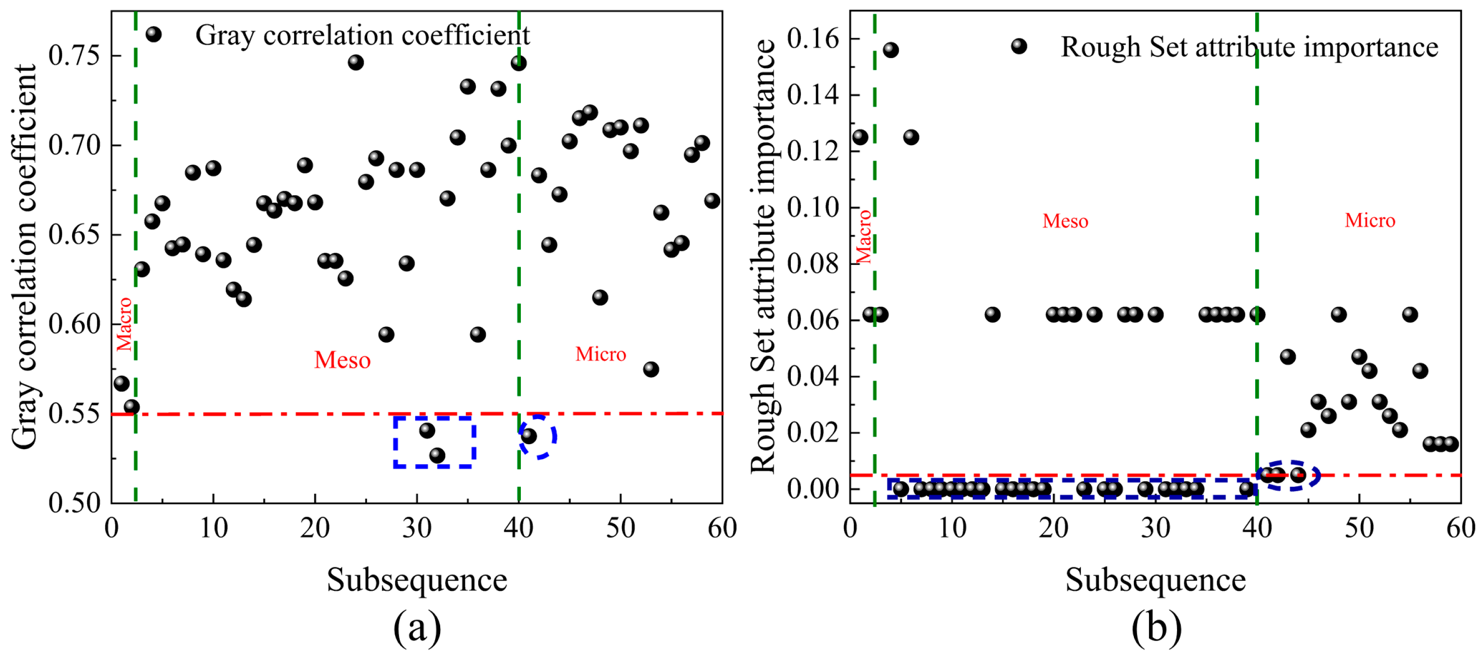
5.2. Parameter Optimization
5.3. Model Prediction of the 34 Optimized Parameters
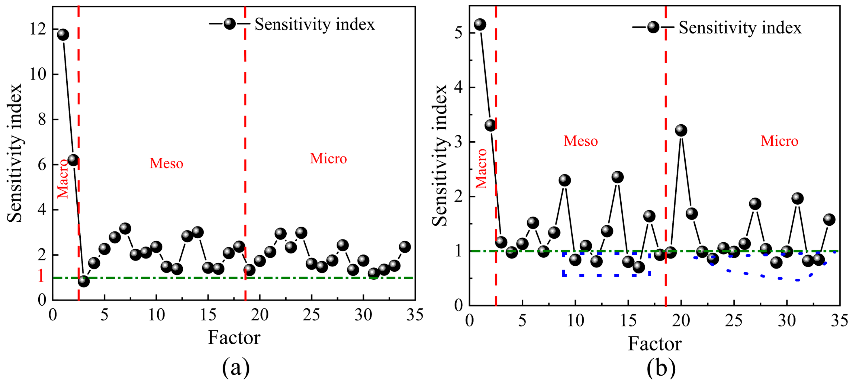
Single Parameter Sensitivity Test of the 34-Parameter Optimal Model
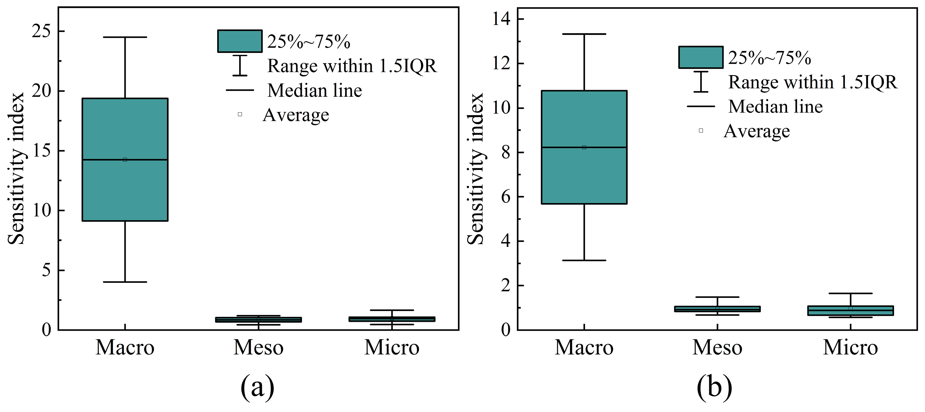
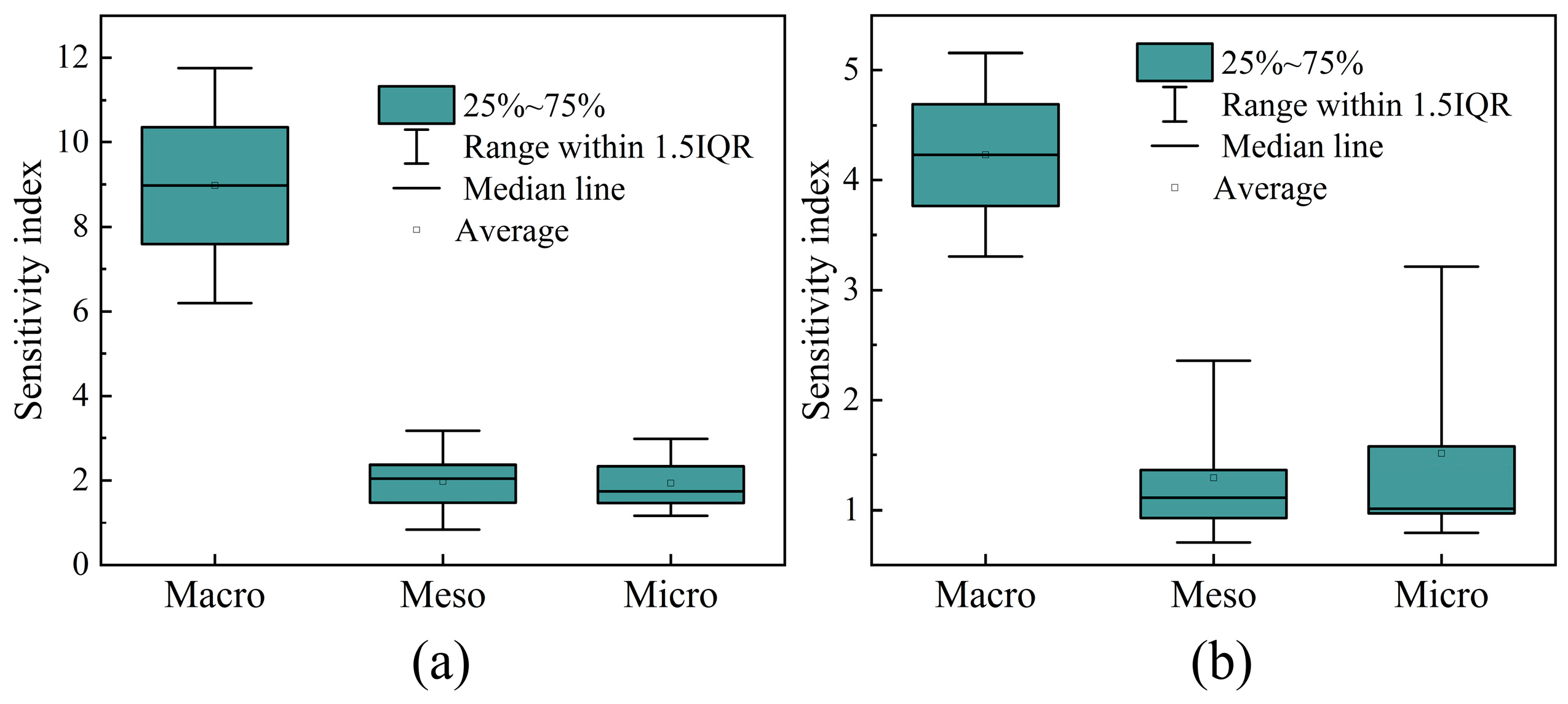
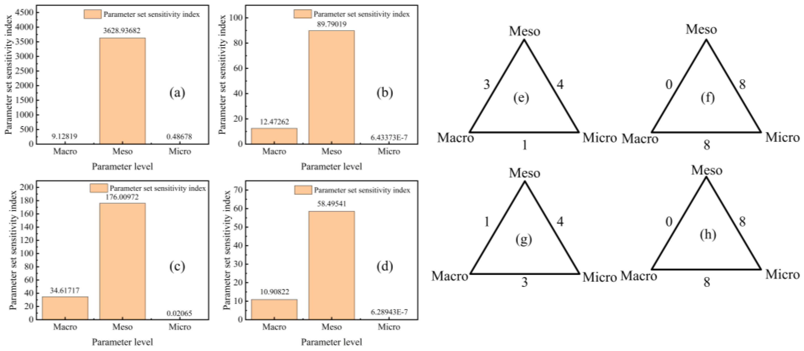
5.4. Sensitivity Analysis of Three-Level Parameter Sets for 59 and 34 Parameter Models
5.5. Model Comparison and Limitation Analysis
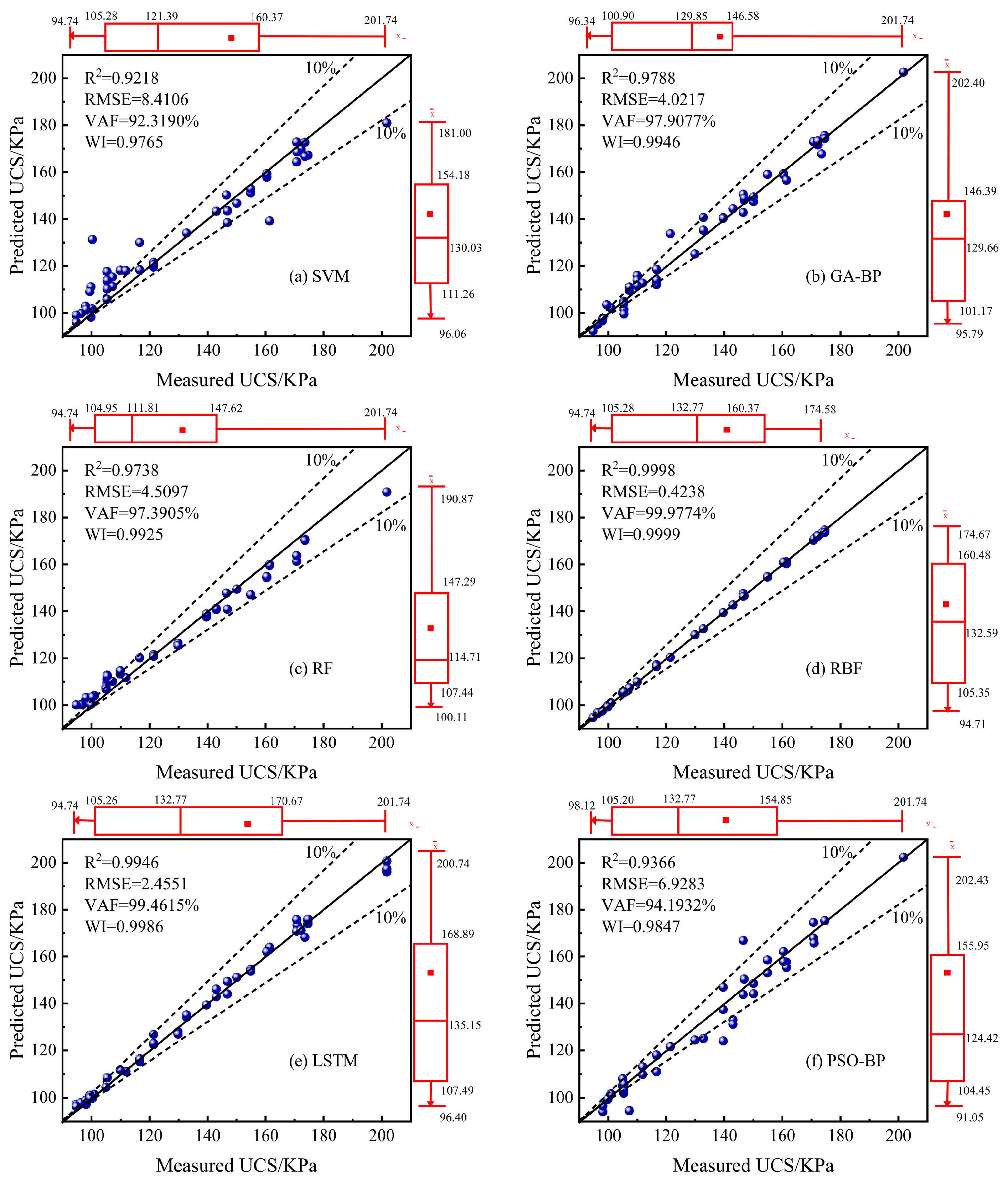
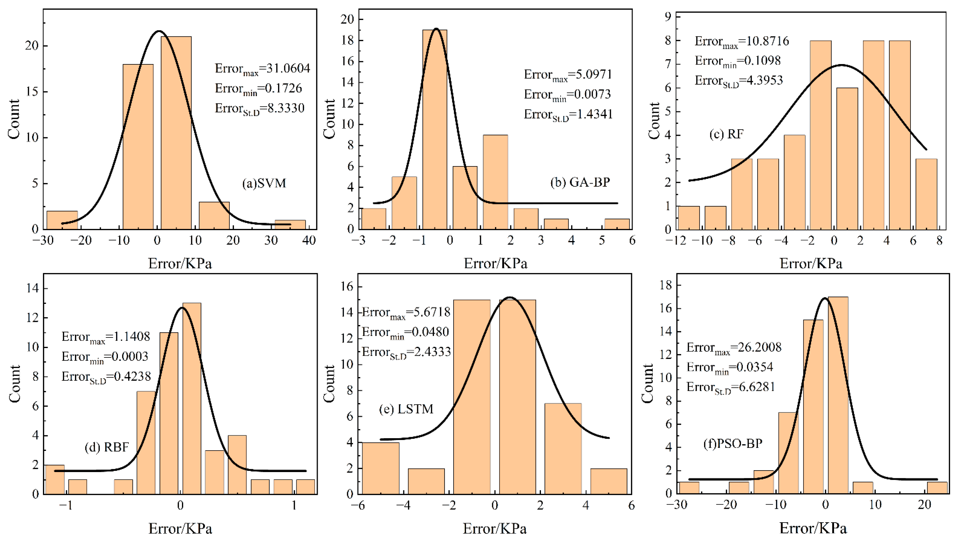
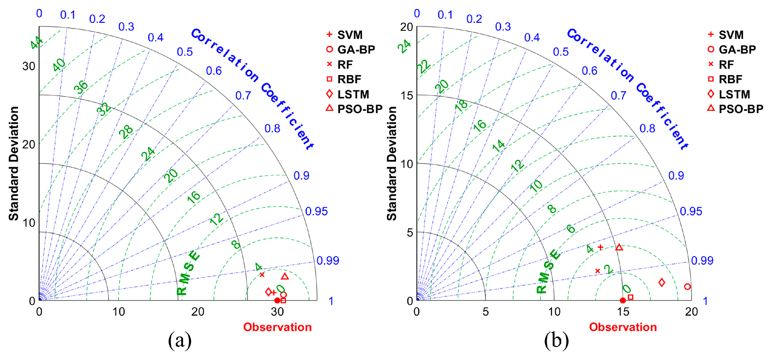
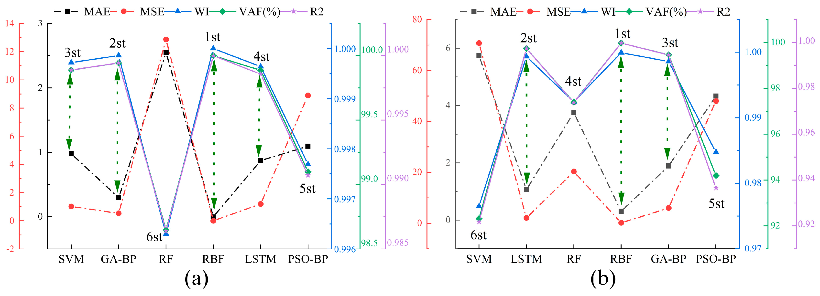
5.5.1. Model Comparison
5.5.2. Analysis of Model Advantages and Limitations
- (1)
- High model accuracy: the overall accuracy of the machine learning model built based on the three-level characteristic interaction hypothesis and the new method of parameter expansion classification is higher; in particular, the optimal model has the highest accuracy.
- (2)
- The model parameters are highly interpretable: the model constructed using the new method has a basis for the expansion and classification of input parameters, and the boundaries between parameters are clear. This greatly increases the interpretability of parameters and can provide a reference for subsequent model parameter selection.
- (3)
- There is a large space for model optimization: the current model is only a preliminary exploration of a new method for expanding and classifying model parameters, and there is a lot of room for optimization. Among them, there is a lot of room for optimization in terms of compressing the number of model parameters, optimizing parameter proportions, simplifying parameter construction, further improving model accuracy, and increasing practicality.
- (1)
- Insufficient model transferability: there are currently relatively few data on multi-level parameters of salinized frozen soil in other literature, so it is impossible to obtain diversified data from different literature to verify the transferability of the constructed model.
- (2)
- The cost of data acquisition is high: the data collection process in the model requires different experiments, which is relatively cumbersome, and the cost of data set acquisition is high.
- (3)
- The parameters are complex and the model is not practical enough: although the number of model parameters has been reduced after parameter optimization, the number of current model parameters is still too large, and the structure is relatively complex, which will increase the difficulty of practical application, thus leading to the model’s insufficient practicality.
- (4)
- There are limitations in the generalizability of the conclusions: the results currently obtained are only applicable to the soil samples used in this study and may not be considered as a general rule for other data sets. It is unclear whether they can be generalized to other soil bodies and other materials.
6. Conclusions and Summary
- (1)
- In the experiment, with the increase in the control factors (number of freeze–thaw cycles, salt content), the macro, meso, and micro parameters all showed obvious stages of characteristics change. Taking the number of freeze–thaw cycles as 5 and 30 as the node, it can be divided into three stages. According to the changes in each stage, the first, second, and third stages are named the adjustment period, the dynamic fluctuation period, and the stable period. The fluctuation characteristics of each stage of the third-level parameters correspond well and show synchronized response characteristics.
- (2)
- The ranking of the six machine learning models in terms of the UCS prediction with 59 parameters is RBF > LSTM > GA-BP > RF > PSO-BP > SVM. The optimal RBF model has the best prediction performance for UCS, with the largest R2, WI, and VAF values and the smallest RMSE value. However, in view of the large difference in the sensitivity distribution of the third-level parameters, the RBF model needs to be further improved.
- (3)
- The massive number of input parameters and obvious proportional differences in the use of the model parameter expansion classification method are the main reasons for the large sensitivity gap of the third-level parameters of the RBF model with 59 parameters. Through gray correlation and rough set analysis between parameters and UCS, optimizing the total number of parameters and the proportion of three-level parameters can effectively solve this problem.
- (4)
- The ranking of the six machine learning models in terms of the UCS prediction with 34 parameters is RBF > LSTM > SVM > GA-BP > RF > PSO-BP, and the optimal model is still RBF. The accuracy and stability of the RBF model are slightly lower, but the sensitivity distribution of the three-level parameters is more reasonable, which can better reflect the macro–meso–micro three-level characteristic response of parameters and is more effective for UCS prediction.
- (5)
- The actual performance of the 59- and 34-parameter models shows that the comprehensive macro–meso–micro three-level characteristic response of the soil can effectively improve the UCS prediction ability of the model. It is proven that it is necessary to expand and classify the input parameters in the soil UCS machine learning model prediction based on the basic hypothesis and basic methods. This approach not only considers the parameters more comprehensively and makes the logical relationship between parameters clearer and more interpretable but also helps to improve the prediction accuracy and stability of the model.
Author Contributions
Funding
Data Availability Statement
Acknowledgments
Conflicts of Interest
References
- Meng, F.D.; Zhai, Y.; Li, Y.B.; Zhao, R.F.; Li, Y.; Gao, H. Research on the effect of pore characteristics on the compressive properties of sandstone after freezing and thawing. Eng. Geol. 2021, 286, 106088. [Google Scholar] [CrossRef]
- Gb/t 50176-2016; Code for Thermal Design of Civil Building. China Planning Press: Beijing, China, 2016; pp. 147–152.
- Lv, Q.F.; Jiang, L.S.; Ma, B.; Zhao, B.H.; Huo, Z.S. A study on the effect of the salt content on the solidification of sulfate saline soil solidified with an alkali-activated geopolymer. Constr. Build. Mater. 2018, 176, 68–74. [Google Scholar] [CrossRef]
- You, Z.; Lai, Y.; Zhang, M.; Liu, E. Quantitative analysis for the effect of microstructure on the mechanical strength of frozen silty clay with different contents of sodium sulfate. Environ. Earth Sci. 2017, 76, 143. [Google Scholar] [CrossRef]
- Li, K.; Li, Q.; Liu, C. Impacts of Water Content and Temperature on the Unconfined Compressive Strength and Pore Characteristics of Frozen Saline Soils. KSCE J. Civ. Eng. 2022, 26, 1652–1661. [Google Scholar] [CrossRef]
- Shen, M.D.; Zhou, Z.W.; Zhang, S.J. Effect of stress path on mechanical behaviours of frozen subgrade soil. Road Mater. Pavement Des. 2022, 23, 1061–1090. [Google Scholar] [CrossRef]
- Wan, X.S.; Lai, Y.M.; Wang, C. Experimental study on the freezing temperatures of saline silty soils. Permafr. Periglac. Process. 2015, 26, 175–187. [Google Scholar] [CrossRef]
- Wallis, S. Freezing under the sea rescues Oslofjord highway tunnel. Tunnel 1999, 8, 19–26. [Google Scholar]
- Wang, H.; Tong, M. Properties and field application of the grouting material for water blocking during thawing of frozen wall of deep sand layer. Arab. J. Geosci. 2021, 14, 1429. [Google Scholar] [CrossRef]
- Zhang, Y.; Yang, Z.H.; Liu, J.K.; Fang, J.H. Impact of cooling on shear strength of high salinity soils. Cold Reg. Sci. Technol. 2017, 141, 122–130. [Google Scholar] [CrossRef]
- Carteret, R.D.; Buzzi, O.; Fityus, S.; Liu, X.F. Effect of naturally occurring salts on tensile and shear strength of sealed granular road pavements. J. Mater. Civ. Eng. 2014, 26, 04014010. [Google Scholar] [CrossRef]
- Xiao, Z.A.; Lai, Y.M.; You, Z.M.; Zhang, M.Y. The phase change process and properties of saline soil during cooling. Arab. J. Sci. Eng. 2017, 42, 3923–3932. [Google Scholar] [CrossRef]
- Lai, Y.M.; Xu, X.T.; Dong, Y.H.; Li, S.Y. Present situation and prospect of mechanical research on frozen soils in China. Cold Reg. Sci. Technol. 2013, 87, 6–18. [Google Scholar] [CrossRef]
- Du, C.C.; Li, D.Q.; Ming, F.; Liu, Y.H.; Shi, X.Y. Wave propagation characteristics in frozen saturated soil. Sci. Cold Arid Reg. 2018, 10, 95–103. [Google Scholar]
- Han, F.H.; Zhang, Z.Q. Properties of 5-year-old concrete containing steel slag powder. Powder Technol. 2018, 334, 27–35. [Google Scholar] [CrossRef]
- Canivell, J.; Martin-del-Rio, J.J.; Alejandre, F.J.; García-Heras, J.; Jimenez-Aguilar, A. Considerations on the physical and mechanical properties of lime-stabilized rammed earth walls and their evaluation by ultrasonic pulse velocity testing. Constr. Build. Mater. 2018, 191, 826–836. [Google Scholar] [CrossRef]
- Martín-del-Rio, J.J.; Canivell, J.; Falcon, R.M. The use of non-destructive testing to evaluate the compressive strength of a lime-stabilised rammed-earth wall: Rebound index and ultrasonic pulse velocity. Constr. Build. Mater. 2020, 242, 118060. [Google Scholar] [CrossRef]
- Wang, J.N.; Huang, L.; Wu, C.Y.; Jiang, T. Mechanical properties and microstructure of saline soil solidified by alkali-activated steel slag. Ceram.–Silikáty 2021, 66, 339–346. [Google Scholar] [CrossRef]
- Choobbasti, A.J.; Samakoosh, M.A.; Kutanaei, S.S. Mechanical properties soil stabilized with nano calcium carbonate and reinforced with carpet waste fibers. Constr. Build. Mater. 2019, 211, 1094–1104. [Google Scholar] [CrossRef]
- Kim, J.; Choi, Y.C.; Choi, S. Fractal characteristics of pore structures in GGBFS-based cement pastes. Appl. Surf. Sci. 2018, 428, 304–314. [Google Scholar] [CrossRef]
- Chen, X.D.; Wu, S.X.; Zhou, J.K. Influence of porosity on compressive and tensile strength of cement mortar. Constr. Build. Mater. 2013, 40, 869–874. [Google Scholar] [CrossRef]
- Atzeni, C.; Pia, G.; Sanna, U. A geometrical fractal model for the porosity and permeability of hydraulic cement pastes. Constr. Build. Mater. 2010, 24, 1843–1847. [Google Scholar] [CrossRef]
- Zhu, Z.D.; Huo, W.W.; Sun, H.; Ma, B.R.; Yang, L. Correlations between unconfined compressive strength, sorptivity and pore structures for geopolymer based on SEM and MIP measurements. J. Build. Eng. 2023, 67, 106011. [Google Scholar] [CrossRef]
- Zhang, X.W.; Kong, L.W.; Yang, A.W.; Sayem, H.M. Thixotropic mechanism of clay: A microstructural investigation. Soils Found. 2017, 57, 23–35. [Google Scholar] [CrossRef]
- Gao, Q.F.; Jrad, M.; Hattab, M.; Fleureau, J.M.; Ameur, L.I. Pore morphology, porosity, and pore size distribution in kaolinitic remolded clays under triaxial loading. Int. J. Geomech. 2020, 20, 04020057. [Google Scholar] [CrossRef]
- Jia, R.; Lei, H.Y.; Li, K. Compressibility and microstructure evolution of different reconstituted clays during 1D compression. Int. J. Geomech. 2020, 20, 04020181. [Google Scholar] [CrossRef]
- Liu, X.Y.; Zhang, X.W.; Kong, L.W.; Wang, G.; Liu, H.H. Formation mechanism of collapsing gully in southern China and the relationship with granite residual soil: A geotechnical perspective. Catena 2022, 210, 105890. [Google Scholar] [CrossRef]
- Zhang, X.W.; Wang, G.; Liu, X.Y.; Xu, Y.Q.; Kong, L.W. Microstructural analysis of pore characteristics of natural structured clay. Bull. Eng. Geol. Environ. 2022, 81, 473. [Google Scholar] [CrossRef]
- Hassanien, A.E.; Darwish, A.; Abdelghafar, S. Machine learning in telemetry data mining of space mission: Basics, challenging and future directions. Artif. Intell. Rev. 2020, 53, 3201–3230. [Google Scholar] [CrossRef]
- Moein, M.M.; Saradar, A.; Rahmati, K.; Mousavinejad, S.H.G.; Bristow, J.; Aramali, V.; Karakouzian, M. Predictive models for concrete properties using machine learning and deep learning approaches: A review. J. Build. Eng. 2023, 63, 105444. [Google Scholar] [CrossRef]
- Baghbani, A.; Choudhury, T.; Costa, S.; Reiner, J. Application of artificial intelligence in geotechnical engineering: A state-of-the-art review. Earth-Sci. Rev. 2022, 228, 103991. [Google Scholar] [CrossRef]
- Dehghanbanadaki, A.; Sotoudeh, M.A.; Golpazir, I.; Keshtkarbanaeemoghadam, A.; Ilbeigi, M. Prediction of geotechnical properties of treated fibrous peat by artificial neural networks. Bull. Eng. Geol. Environ. 2019, 78, 1345–1358. [Google Scholar] [CrossRef]
- Eyo, E.U.; Abbey, S.J. Machine learning regression and classification algorithms utilised for strength prediction of OPC/by-product materials improved soils. Constr. Build. Mater. 2021, 284, 122817. [Google Scholar] [CrossRef]
- Ngo, A.Q.; Nguyen, L.Q.; Tran, V.Q. Developing interpretable machine learning-Shapley additive explanations model for unconfined compressive strength of cohesive soils stabilized with geopolymer. PLoS ONE 2023, 18, e0286950. [Google Scholar] [CrossRef] [PubMed]
- Shafiei, A.; Aminpour, M.; Hasanzadehshooiili, H.; Ghorbani, A.; Nazem, M. Mechanical characterization of marl soil treated by cement and lignosulfonate under freeze-thaw cycles: Experimental studies and machine-learning modeling. Bull. Eng. Geol. Environ. 2023, 82, 200. [Google Scholar] [CrossRef]
- Zeini, H.A.; Al-Jeznawi, D.; Imran, H.; Bernardo, L.F.A.; Al-Khafaji, Z.; Ostrowski, K.A. Random Forest Algorithm for the Strength Prediction of Geopolymer Stabilized Clayey Soil. Sustainability 2023, 15, 1408. [Google Scholar] [CrossRef]
- Eyo, E.U.; Abbey, S.J.; Booth, C.A. Strength predictive modelling of soils treated with calcium-based additives blended with eco-friendly pozzolans-A machine learning approach. Materials 2022, 15, 4575. [Google Scholar] [CrossRef] [PubMed]
- Tran, V.Q. Hybrid gradient boosting with meta-heuristic algorithms prediction of unconfined compressive strength of stabilized soil based on initial soil properties, mix design and effective compaction. J. Clean. Prod. 2022, 355, 131683. [Google Scholar] [CrossRef]
- Zhang, G.B.; Ding, Z.Q.; Wang, Y.F.; Fu, G.H.; Wang, Y.; Xie, C.F.; Zang, Y.; Zhao, X.; Lu, X.Y.; Wang, X.Y. Performance Prediction of Cement Stabilized Soil Incorporating Solid Waste and Propylene Fiber. Materials 2022, 15, 4250. [Google Scholar] [CrossRef]
- Bing, H.; Zhang, Y.; Ma, M. Impact of desalination on physical and mechanical properties of Lanzhou loess. Eurasian Soil Sci. 2017, 50, 1444–1449. [Google Scholar] [CrossRef]
- Lai, Y.; Liao, M.; Hu, K. A constitutive model of frozen saline sandy soil based on energy dissipation theory. Int. J. Plast. 2016, 78, 84–113. [Google Scholar] [CrossRef]
- ASTM D2487–17; Standard Practice for Classification of Soils for Engineering Purposes (Unified Soil Classification System). ASTM International: West Conshohocken, PA, USA, 2020.
- ASTM-D560/D560M; Standard Test Methods for Freezing and Thawing Com-Pacted Soil-Cement Mixtures. ASTM International: West Conshohocken, PA, USA, 2016.
- ASTM-D2166; Standard Test Method for Unconfined Compressive Strength of Cohesive Soil. ASTM International: West Conshohocken, PA, USA, 2016.
- Brignoli, E.G.; Gotti, M.; Stokoe, K.H. Measurement of shear waves in laboratory specimens by means of piezoelectric transducers. Geotech. Test. J. 1996, 19, 384–397. [Google Scholar]
- Leong, E.C.; Cahyadi, J.; Rahardjo, H. Measuring shear and compression wave velocities of soil using bender–extender elements. Can. Geotech. J. 2009, 46, 792–812. [Google Scholar] [CrossRef]
- Liu, C.; Shi, B.; Zhou, J.; Tang, C. Quantification and characterization of microporosity by image processing, geometric measurement and statistical methods: Application on SEM images of clay materials. Appl. Clay Sci. 2011, 54, 97–106. [Google Scholar] [CrossRef]
- Liu, C.; Tang, C.S.; Shi, B.; Suo, W.B. Automatic quantification of crack patterns by image processing. Comput. Geosci. 2013, 57, 77–80. [Google Scholar] [CrossRef]
- Gu, K.; Shi, B.; Liu, C.; Jiang, H.; Li, T.; Wu, J. Investigation of land subsidence with the combination of distributed fiber optic sensing techniques and microstructure analysis of soils. Eng. Geol. 2018, 240, 34–47. [Google Scholar] [CrossRef]
- Tang, C.S.; Lin, L.; Cheng, Q.; Zhu, C.; Wang, D.W.; Lin, Z.Y.; Shi, B. Quantification and characterizing of soil microstructure features by image processing technique. Comput. Geotech. 2020, 128, 103817. [Google Scholar] [CrossRef]
- Liu, X.; Deng, W.; Wang, S.; Liu, B.; Liu, Q. Experimental investigation on microstructure and surface morphology deterioration of limestone exposed on acidic environment. Constr. Build. Mater. 2023, 377, 131065. [Google Scholar] [CrossRef]
- Tang, C.; Shi, B.; Liu, C.; Zhao, L.; Wang, B. Influencing factors of geometrical structure of surface shrinkage cracks in clayey soils. Eng. Geol. 2008, 101, 204–217. [Google Scholar] [CrossRef]
- Jiang, N.; Li, H.; Liu, Y.; Li, H.; Wen, D. Pore microstructure and mechanical behaviour of frozen soils subjected to variable temperature. Cold Reg. Sci. Technol. 2023, 206, 103740. [Google Scholar] [CrossRef]
- Lawal, A.I.; Idris, M.A. An artificial neural network-based mathematical model for the prediction of blast-induced ground vibrations. Int. J. Environ. Stud. 2020, 77, 318–334. [Google Scholar] [CrossRef]
- Somvanshi, M.; Chavan, P.; Tambade, S.; Shinde, S.V. A review of machine learning techniques using decision tree and support vector machine. In Proceedings of the 2016 International Conference on Computing Communication Control and Automation (ICCUBEA), Pune, India, 12–13 August 2016; pp. 1–7. [Google Scholar] [CrossRef]
- Liu, Y.Q.; Jiang, C.Q.; Lu, C.P.; Wang, Z.; Che, W.L. Increasing the Accuracy of Soil Nutrient Prediction by Improving Genetic Algorithm Backpropagation Neural Networks. Symmetry 2023, 15, 151. [Google Scholar] [CrossRef]
- Liu, D.W.; Liu, C.; Tang, Y.; Gong, C. A GA-BP neural network regression model for predicting soil moisture in slope ecological protection. Sustainability 2022, 14, 1386. [Google Scholar] [CrossRef]
- Dai, Y.; Khandelwal, M.; Qiu, Y.G.; Zhou, J.; Monjezi, M.; Yang, P.X. A hybrid metaheuristic approach using random forest and particle swarm optimization to study and evaluate backbreak in open-pit blasting. Neural Comput. Appl. 2022, 34, 6273–6288. [Google Scholar] [CrossRef]
- Zhang, P.; Yin, Z.Y.; Jin, Y.F.; Chan, T.H.T. A novel hybrid surrogate intelligent model for creep index prediction based on particle swarm optimization and random forest. Eng. Geol. 2020, 265, 105328. [Google Scholar] [CrossRef]
- Imanian, H.; Shirkhani, H.; Mohammadian, A.; Cobo, J.H.; Payeur, P. Spatial interpolation of soil temperature and water content in the land-water interface using artificial intelligence. Water 2023, 15, 473. [Google Scholar] [CrossRef]
- Huo, D.Y.; Chen, J.S.; Zhang, H.; Shi, Y.R.; Wang, T.Y. Intelligent prediction for digging load of hydraulic excavators based on RBF neural network. Measurement 2023, 206, 112210. [Google Scholar] [CrossRef]
- Bui, D.T.; Prakash, I.A. Sustainable Development of Urban Underground Space Using Deep Learning Method Based on LSTM at Substation Site in Southern Vietnam. In Lecture Notes in Civil Engineering; Springer: Berlin/Heidelberg, Germany, 2021; Volume 187, pp. 127–142. [Google Scholar]
- Zamani, M.G.; Nikoo, M.R.; Rastad, D.; Nematollahi, B. A comparative study of data-driven models for runoff, sediment, and nitrate forecasting. J. Environ. Manag. 2023, 341, 118006. [Google Scholar] [CrossRef] [PubMed]
- Huang, F.N.; Zhang, Y.K.; Zhang, Y.; Shangguan, W.; Li, Q.L.; Li, L.; Jiang, S.J. Interpreting Conv-LSTM for Spatio-Temporal Soil Moisture Prediction in China. Agriculture 2023, 13, 971. [Google Scholar] [CrossRef]
- Mulumba, D.M.; Liu, J.K.; Hao, J.; Zheng, Y.N.; Liu, H.Q. Application of an Optimized PSO-BP Neural Network to the Assessment and Prediction of Underground Coal Mine Safety Risk Factors. Appl. Sci. 2023, 13, 5317. [Google Scholar] [CrossRef]
- Wang, X.F.; Dong, X.P.; Zhang, Z.S.; Zhang, J.M.; Ma, G.W.; Yang, X. Compaction quality evaluation of subgrade based on soil characteristics assessment using machine learning. Transp. Geotech. 2022, 32, 100703. [Google Scholar] [CrossRef]
- Fallahi, S.; Taghadosi, M. Quantum-behaved particle swarm optimization based on solitons. Sci. Rep. 2022, 12, 13977. [Google Scholar] [CrossRef] [PubMed]
- Benemaran, R.S.; Esmaeili-Falak, M. Predicting the Young’s modulus of frozen sand using machine learning approaches: State-of-the-art review. Geomech. Eng. 2023, 34, 507–527. [Google Scholar] [CrossRef]
- Kardani, N.; Aminpour, M.; Raja, M.N.A.; Kumar, G.; Bardhan, A.; Nazem, M. Prediction of the resilient modulus of compacted subgrade soils using ensemble machine learning methods. Transp. Geotech. 2022, 36, 100827. [Google Scholar] [CrossRef]
- Yu, Z.; Shi, X.Z.; Zhou, J.; Gou, Y.G.; Huo, X.F.; Zhang, J.H.; Armaghani, D.J. A new multikernel relevance vector machine based on the HPSOGWO algorithm for predicting and controlling blast-induced ground vibration. Eng. Comput. 2022, 38, 1905–1920. [Google Scholar] [CrossRef]
- Roshan, M.J.; Rashid, A.S.A.; Wahab, N.A.; Tamassoki, S.; Jusoh, S.N.; Hezmi, M.A.; Daud, N.N.N.; Apandi, N.M.; Azmi, M. Improved methods to prevent railway embankment failure and subgrade degradation: A review. Transp. Geotech. 2022, 37, 100834. [Google Scholar] [CrossRef]
- Rebouh, R.; Boukhatem, B.; Ghrici, M.; Tagnit-Hamou, A. A practical hybrid NNGA system for predicting the compressive strength of concrete containing natural pozzolan using an evolutionary structure. Constr. Build. Mater. 2017, 149, 778–789. [Google Scholar] [CrossRef]
- Liong, S.Y.; Lim, W.H.; Paudyal, G.N. River stage forecasting in Bangladesh: Neural network approach. J. Comput. Civ. Eng. 2000, 14, 1–8. [Google Scholar] [CrossRef]
- Suthar, M. Applying several machine learning approaches for prediction of unconfined compressive strength of stabilized pond ashes. Neural Comput. Appl. 2020, 32, 9019–9028. [Google Scholar] [CrossRef]
- Tong, S.C.; Li, G.R.; Li, X.L.; Li, J.F.; Zhai, H.; Zhao, J.Y.; Zhu, H.L.; Liu, Y.B.; Chen, W.T.; Hu, X.S. Soil Water Erosion and Its Hydrodynamic Characteristics in Degraded Bald Patches of Alpine Meadows in the Yellow River Source Area, Western China. Sustainability 2023, 15, 8165. [Google Scholar] [CrossRef]
- Yao, M.; Wang, Q.; Yu, Q.B.; Wu, J.Z.; Li, H.; Dong, J.Q.; Xia, W.T.; Han, Y.; Huang, X.L. Mechanism Study of Differential Permeability Evolution and Microscopic Pore Characteristics of Soft Clay under Saturated Seepage: A Case Study in Chongming East Shoal. Water 2023, 15, 968. [Google Scholar] [CrossRef]
- Wong, M.; Parker, G. Reanalysis and correction of bed-load relation of Meyer-Peter and Müller using their own database. J. Hydraul. Eng. 2006, 132, 1159–1168. [Google Scholar] [CrossRef]
- Ang, J.C.; Tang, J.Y.; Chung, B.Y.H.; Chong, J.W.; Tan, R.R.; Aviso, K.B.; Chemmangattuvalappil, N.G.; Thangalazhy-Gopakumar, S. Development of predictive model for biochar surface properties based on biomass attributes and pyrolysis conditions using rough set machine learning. Biomass Bioenergy 2023, 174, 106820. [Google Scholar] [CrossRef]
- Nofalah, M.H.; Ghadir, P.; Hasanzadehshooiili, H.; Aminpour, M.; Javadi, A.A.; Nazem, M. Effects of binder proportion and curing condition on the mechanical characteristics of volcanic ash-and slag-based geopolymer mortars; machine learning integrated experimental study. Constr. Build. Mater. 2023, 395, 132330. [Google Scholar] [CrossRef]
- Ahenkorah, I.; Rahman, M.M.; Karim, M.R.; Beecham, S. Unconfined compressive strength of MICP and EICP treated sands subjected to cycles of wetting-drying, freezing-thawing and elevated temperature: Experimental and EPR modelling. J. Rock. Mech. Geotech. 2023, 15, 1226–1247. [Google Scholar] [CrossRef]
- Taffese, W.Z.; Abegaz, K.A. Prediction of compaction and strength properties of amended soil using machine learning. Buildings 2022, 12, 613. [Google Scholar] [CrossRef]
- Soleimani, S.; Rajaei, S.; Jiao, P.; Sabz, A.; Soheilinia, S. New prediction models for unconfined compressive strength of geopolymer stabilized soil using multi-gen genetic programming. Measurement 2018, 113, 99–107. [Google Scholar] [CrossRef]
- Tinoco, J.; Alberto, A.; Venda, P.; Correia, A.G.; Lemos, L.A. data-driven approach for qu prediction of laboratory soil-cement mixtures. Procedia Eng. 2016, 143, 566–573. [Google Scholar] [CrossRef]
- Mozumder, R.A.; Laskar, A.I.; Hussain, M. Empirical approach for strength prediction of geopolymer stabilized clayey soil using support vector machines. Constr. Build. Mater. 2017, 132, 412–424. [Google Scholar] [CrossRef]
- Ghorbani, A.; Hasanzadehshooiili, H. Prediction of UCS and CBR of microsilica-lime stabilized sulfate silty sand using ANN and EPR models; application to the deep soil mixing. Soils Found. 2018, 58, 34–49. [Google Scholar] [CrossRef]
- Suman, S.; Mahamaya, M.; Das, S.K. Prediction of maximum dry density and unconfined compressive strength of cement stabilised soil using artificial intelligence techniques. Int. J. Geosynth. Ground Eng. 2016, 2, 11. [Google Scholar] [CrossRef]
- Tiwari, N.; Satyam, N. Coupling effect of pond ash and polypropylene fiber on strength and durability of expansive soil subgrades: An integrated experimental and machine learning approach. J. Rock. Mech. Geotech. 2021, 13, 1101–1112. [Google Scholar] [CrossRef]


| Model | Input Parameters | Soil Type | Performance | Reference |
|---|---|---|---|---|
| BP; PSO-BP | 5 | Treated fibrous peat soil | BP: R = 0.928; MSE = 2.14 PSO-BP: R = 1.000; MSE = 0.73 | Dehghanbanadaki et al. [32] |
| REG; RDF; BLR | 5 | Soil improvement such as OPT | REG: R2 = 0.91; RMSE = 0.31 RDF: R2 = 0.89; RMSE = 0.34 BLR: R2 = 0.91; RMSE = 0.31 | Eyo and Abbey. [33] |
| ANN | 8 | Cohesive soils stabilized with geopolymer | R2 = 0.9808; RMSE = 0.8808 | Ngo et al. [34] |
| KNN; XGB | 4 | Marl soil treated by cement and lignosulfonate | KNN: R2 = 0.811; RMSE = 151.408 XGB: R2 = 0.954; RMSE = 74.878 | Shafiei et al. [35] |
| RF | 7 | Geopolymer stabilized clayey soil | R2 = 0.9757; RMSE = 0.9815 | Zeini et al. [36] |
| GB-ML | 8 | TCEF-soils | R2 = 0.900; RMSE = 0.335 | Eyo et al. [37] |
| GB-PSO | 12 | Australia-EBCA-soils | R2 = 0.9655; RMSE = 0.1633 | Tran. [38] |
| BAS-BP | 5 | CPF soils | R = 0.9594; RMSE = 0.1727 | Zhang et al. [39] |
| Cation Content/% | Anion Content/% | Total Salt Content/% | ||||||
|---|---|---|---|---|---|---|---|---|
| Na+ | K+ | Mg2+ | Ca2+ | Cl− | SO4−2 | NO3− | ||
| Before | 0.2355 | 0.0036 | 0.0238 | 0.1624 | 0.1144 | 0.7756 | 0.0020 | 1.3173 |
| After | 0.0058 | 0.0013 | 0.0022 | 0.0142 | 0.0021 | 0.0095 | 0.0001 | 0.0352 |
| Physical Index | % | % | % | cm−3 | % | Specific Gravity of Soil | g−1 |
|---|---|---|---|---|---|---|---|
| Value | 8.38 | 33.38 | 24.99 | 1.68 | 12.64 | 2.71 | 4.86 |
| Stage | Macro | Meso | Micro |
|---|---|---|---|
| Stage 1: Adjustment period | I: A1; B1 | * I: (A1); (C1) * II: (A1); (B2) | ** I: <A1>; <B1> ** II: <A1>; <B1> ** III: <A1>; <C1> ** IV: <A1>; <B1> |
| Stage 2: Dynamic fluctuation period | I: A2; B2 | * I: (A2); (B2) * II: (A2); (B1) | ** I: <A2>; <B2> ** II: <A2>; <C2> ** III: <A2>; <D2>; <F2> ** IV: <A2>; <E2>; <F2> |
| Stage 3: Stable period | I: A3; B3 | * I: (A3); (B3) * II: (A3); (B3) | ** I: <A3>; <B3> ** II: <A3>; <B3> ** III: <A3>; <C3>; <D3> ** IV: <A3>; <C3> |
| Parameter code | X1 | X2 |
| Definition | S | N |
| Parameter code | X3 | X4 | X5 | X6 |
| Definition |
| Parameter Code | Definition | Parameter Code | Definition | Parameter Code | Definition |
|---|---|---|---|---|---|
| X7 | X19 | X31 | |||
| X8 | X20 | X32 | |||
| X9 | X21 | X33 | |||
| X10 | X22 | X34 | |||
| X11 | X23 | X35 | |||
| X12 | X24 | X36 | |||
| X13 | X25 | X37 | |||
| X14 | X26 | X38 | |||
| X15 | X27 | X39 | |||
| X16 | X28 | X40 | |||
| X17 | X29 | ||||
| X18 | X30 |
| Parameter Code | Definition | Parameter Code | Definition | Parameter Code | Definition |
|---|---|---|---|---|---|
| X41 | Image area | X48 | Average form factor | X55 | APDI |
| X42 | Total region area | X49 | Maxima length | X56 | PPDFD |
| X43 | Region number | X50 | Average length | X57 | Sorting Coefficient |
| X44 | Region percentage | X51 | Maxima width | X58 | UC |
| X45 | Maxima region area | X52 | Average width | X59 | Curvature Coefficient |
| X46 | Average region area | X53 | Probability Entropy | ||
| X47 | Average perimeter | X54 | Fractal dimension |
| Columns | Macro Parameters | Meso Parameters | Micro Parameters | UCS | |
|---|---|---|---|---|---|
| Rows | |||||
| 1–32 | A | B | C1 | D | |
| 33–64 | A | B | C2 | D | |
| 65–96 | A | B | C3 | D | |
| 97–128 | A | B | C4 | D | |
| 129–160 | A | B | C5 | D | |
| 161–192 | A | B | C6 | D | |
| Variables | Unite | Symbol | Mean | Max | Min | St.D | Sk | Ku |
|---|---|---|---|---|---|---|---|---|
| UCS | kPa | UCS | 131.21 | 201.73 | 94.73 | 30.20 | 0.46 | −1.10 |
| S | % | X1 | 0.87 | 2 | 0 | 0.73 | 0.43 | −1.16 |
| N | 1 | X2 | 14.87 | 50 | 0 | 16.45 | 1.08 | −0.09 |
| VS1 | km/s | X3 | 0.15 | 0.19 | 0.13 | 0.01 | 0.89 | −0.05 |
| VS2 | km/s | X4 | 0.16 | 0.18 | 0.14 | 0 | −0.64 | −0.04 |
| VP1 | km/s | X5 | 0.2 | 0.25 | 0.18 | 0.01 | 0.92 | 0.31 |
| VP2 | km/s | X6 | 0.19 | 0.19 | 0.16 | 0.01 | −0.35 | −0.27 |
| km/s | X7 | 0.01 | 0.06 | 0 | 0.01 | 0.81 | 0.05 | |
| km/s | X8 | 0.01 | 0.04 | 0 | 0 | 1.08 | 1.8 | |
| 1 | X9 | 0.08 | 0.26 | 0 | 0.06 | 0.63 | −0.33 | |
| 1 | X10 | 0.08 | 0.34 | 0 | 0.07 | 1.5 | 3.38 | |
| 1 | X11 | 1.19 | 1.37 | 1.04 | 0.08 | 0.24 | −0.67 | |
| km/s | X12 | 0.03 | 0.05 | 0 | 0.01 | 0.04 | −0.92 | |
| km/s | X13 | 0.01 | 0.04 | 0 | 0.01 | 0.97 | 0.59 | |
| km2/s2 | X14 | 0.03 | 0.05 | 0.02 | 0 | −0.17 | −0.29 | |
| km2/s2 | X15 | 0.02 | 0.03 | 0.01 | 0 | −0.51 | −0.18 | |
| km2/s2 | X16 | 0 | 0 | 0 | 0 | 2.28 | 5.7 | |
| km2/s2 | X17 | 0 | 0 | 0 | 0 | 3.28 | 12.7 | |
| GPa | X18 | 0.05 | 0.06 | 0.03 | 0 | −0.51 | −0.18 | |
| 1 | X19 | 1.02 | 4.46 | 0.05 | 1 | 1.77 | 2.82 | |
| km2/s2 | X20 | 0.04 | 0.06 | 0.03 | 0 | 1.09 | 0.56 | |
| km2/s2 | X21 | 0.02 | 0.03 | 0.01 | 0 | 1.03 | 0.15 | |
| GPa | X22 | 0.04 | 0.07 | 0.03 | 0 | 1.03 | 0.15 | |
| 1 | X23 | 0.19 | 0.56 | 0.01 | 0.13 | 0.89 | 0.44 | |
| GPa | X24 | 0.43 | 2.09 | 0 | 0.56 | 1.82 | 2.36 | |
| GPa | X25 | 0 | 0.02 | 0 | 0 | 1 | 1.48 | |
| 1 | X26 | 0.84 | 4.28 | 0 | 0.99 | 1.83 | 2.91 | |
| 1 | X27 | 0.84 | 1.22 | 0.02 | 0.3 | −1.16 | 0. | |
| 1 | X28 | 0.18 | 0.8 | 0 | 0.16 | 1.84 | 4.8 | |
| 1 | X29 | 0.15 | 0.45 | 0 | 0.12 | 0.43 | −0.72 | |
| 1 | X30 | 0.18 | 0.8 | 0 | 0.16 | 1.84 | 4.8 | |
| 1 | X31 | 0.98 | 1 | 0.93 | 0.01 | −2.02 | 4.29 | |
| 1 | X32 | 0.98 | 1 | 0.88 | 0.02 | −3.84 | 16. | |
| 1 | X33 | 0.29 | 1.46 | 0 | 0.38 | 1.99 | 3.02 | |
| 1 | X34 | 1.11 | 1.8 | 0.77 | 0.21 | 0.92 | 1.43 | |
| 1 | X35 | 8.59 | 37.88 | 0.84 | 9.19 | 1.45 | 1.6 | |
| 1 | X36 | 0.84 | 1.22 | 0.02 | 0.3 | −1.16 | 0.7 | |
| 1 | X37 | 0.18 | 0.8 | 0 | 0.16 | 1.84 | 4.8 | |
| 1 | X38 | 7.73 | 36.88 | 0.03 | 9.38 | 1.44 | 1.51 | |
| GPa | X39 | 0.09 | 0.66 | 0 | 0.14 | 2.7 | 7.16 | |
| GPa | X40 | 0.49 | 2.27 | 0.03 | 0.58 | 1.69 | 1.77 | |
| Image area | pixel | X41 | 1,569,032 | 1,574,400 | 1,545,216 | 5522.56 | −3.34 | 11.16 |
| Total region area | X42 | 348,390.76 | 854,526 | 121,255 | 68,664.57 | 3.41 | 24.31 | |
| Region number | 1 | X43 | 848.65 | 1542 | 159 | 255.59 | 0.06 | 0.07 |
| Region percentage | % | X44 | 7.67 | 54.38 | 0.19 | 11.36 | 1.3 | 1.09 |
| Max region area | X45 | 56,331.4 | 295,866 | 9333 | 44,069.51 | 2.41 | 8.29 | |
| Average region area | X46 | 453.75 | 1357.64 | 227.57 | 183.62 | 2.1 | 5.92 | |
| Average perimeter | X47 | 98.08 | 146.84 | 78.67 | 11.38 | 1.05 | 1.58 | |
| Average form factor | 1 | X48 | 0.38 | 0.42 | 0.33 | 0.01 | −0.45 | 0.14 |
| Max length | X49 | 498.44 | 1447.68 | 200.48 | 199.56 | 1.45 | 3.35 | |
| Average length | X50 | 27.14 | 35.47 | 23.21 | 2.24 | 0.97 | 1.07 | |
| Max width | X51 | 281.62 | 662 | 99.61 | 103.78 | 1.05 | 1.21 | |
| Average width | X52 | 15.51 | 19.84 | 13.46 | 1.11 | 0.85 | 0.95 | |
| Probability Entropy | 1 | X53 | 0.98 | 0.99 | 0.96 | 0 | −1.91 | 6.2 |
| Fractal dimension | 1 | X54 | 1.19 | 1.26 | 1.14 | 0.02 | 0.26 | −0.07 |
| APDI | 1 | X55 | 1.98 | 2.28 | 1.7 | 0.11 | 0.23 | −0.49 |
| PPDFD | 1 | X56 | 1.97 | 2.54 | 1.43 | 0.2 | 0.17 | −0.1 |
| Sorting Coefficient | 1 | X57 | 1.39 | 4.69 | 1.05 | 0.35 | 5.67 | 44.18 |
| Uniformity Coefficient | 1 | X58 | 1.75 | 4.54 | 1.09 | 0.38 | 2.36 | 13.56 |
| Curvature Coefficient | 1 | X59 | 1.18 | 2.26 | 0.41 | 0.26 | 1.86 | 5.2 |
| Model | Hyperparameter |
|---|---|
| SVM | PF = 4.0; RP = 0.8 |
| GA-BP | NI = 105; ET = 10−6; LR = 10−2; NH = 7; GA = 50; PS = 5 |
| RF | NDT =100; MNL = 5 |
| RBF | ESR = 100 |
| LSTM | LL = 4; MNI = 1200; ILA = 10−2; LIDF = 0.5 |
| PSO-BP | NI = 105; ET = 10−6; LR = 10−2; NH = 7; LF = 4.494; NPU = 30; PS = 5 |
| Model | Performance | and | Rank | Total | |||||
|---|---|---|---|---|---|---|---|---|---|
| R2 | Score | RMSE | Score | WI | Score | VAF (%) | Score | ||
| SVM | 0.9989 | 4 | 1.0094 | 4 | 0.9997 | 4 | 99.8886 | 4 | 16 |
| GA-BP | 0.9994 | 5 | 0.7286 | 5 | 0.9999 | 5 | 99.9438 | 5 | 20 |
| RF | 0.9864 | 1 | 3.5871 | 1 | 0.9963 | 1 | 98.6484 | 1 | 4 |
| RBF | 1 | 6 | 3.79 × 10⁻⁷ | 6 | 1 | 6 | 100 | 6 | 24 |
| LSTM | 0.9985 | 3 | 1.0931 | 3 | 0.9996 | 3 | 99.8869 | 3 | 12 |
| PSO-BP | 0.9907 | 2 | 2.9826 | 2 | 0.9977 | 2 | 99.0997 | 2 | 8 |
| Model | Performance | and | Rank | Total | |||||
|---|---|---|---|---|---|---|---|---|---|
| R2 | Score | RMSE | Score | WI | Score | VAF (%) | Score | ||
| SVM | 0.9218 | 1 | 8.4106 | 1 | 0.9765 | 1 | 92.3190 | 1 | 4 |
| GA-BP | 0.9788 | 4 | 4.0217 | 4 | 0.9946 | 4 | 97.9077 | 4 | 16 |
| RF | 0.9738 | 3 | 4.5067 | 3 | 0.9925 | 3 | 97.3905 | 3 | 12 |
| RBF | 0.9998 | 6 | 0.4238 | 6 | 0.9999 | 6 | 99.9774 | 6 | 24 |
| LSTM | 0.9946 | 5 | 2.4451 | 5 | 0.9986 | 5 | 99.4615 | 5 | 20 |
| PSO-BP | 0.9366 | 2 | 6.9283 | 2 | 0.9847 | 2 | 94.1932 | 2 | 8 |
| Type | Quantity | Specific |
|---|---|---|
| Macro | 2 | X1; X2 |
| Meso | 16 | X3; X4; X6; X14; X20; X21; X22; X24; X27; X28; X30; X35; X36; X37; X38; X40 |
| Micro | 16 | X43; X45; X46; X47; X48; X49; X50; X51; X52; X53; X54; X55; X56; X57; X58; X59 |
| Stage | R2 | RMSE | WI | VAF (%) |
|---|---|---|---|---|
| Training | 1 | 1.37 × 10⁻⁵ | 1 | 100 |
| Testing | 0.9868 | 3.7166 | 0.9967 | 98.8338 |
| Model | Soil | Parameters | Parameter Type | Performance | References |
|---|---|---|---|---|---|
| Before parameter optimization: SVM; GA-BP; RF; RBF; LSTM; PSO-BP | Saline soil in Lanzhou, China | 59 | Macro–meso–micro | SVM: R2 = 0.9218; RMSE = 8.4160; GA-BP: R2 = 0.9788; RMSE = 4.0217; RF: R2 = 0.9738; RMSE = 4.5067; RBF: R2 = 0.9998; RMSE = 0.4238; LSTM: R2 = 0.9946; RMSE = 2.4451; PSO-BP: R2 = 0.9366; RMSE = 6.9283; | This article |
| After parameter optimization: RBF | Saline soil in Lanzhou, China | 34 | Macro–meso–micro | RBF: R2 = 0.9868; RMSE = 3.7166; | This article |
| EPR modelling A; B; C | Adelaide Industrial (AI) sand | 1; 4; 4 | All macro | EPR-A: R2 = 0.714; RMSE = 1.461; EPR-B: R2 = 0.885; RMSE = 0.374; EPR-C: R2 = 0.939; RMSE = 0.273; | Ahenkorah et al. [80] |
| OEM; ANNs | Soils from around the world | 9 | All macro | OEM: R2 = 0.61; MSE = 370,860; ANNs: R2 = 0.65; MSE = 457,271; | Taffese and Abegaz. [81] |
| MGGP; ANNs | Geopolymer-stabilized clayey soil | 9 | All macro | MGGP: R2 = 0.942; MSE = 2.366; ANNs: R2 = 0.964; MSE = 1.500; | Soleimani et al. [82] |
| MR; ANNs; SVM | The soils selected were from Coimbra area | 8 | All macro | MR: R2 = 0.59; RMSE = 0.56; ANNs: R2 = 0.91; RMSE = 0.26; SVM: R2 = 0.93; RMSE = 0.23; | Tinoco et al. [83] |
| ERBF; RBF; POLY | Three different types of clayey soil | 7 | All macro | ERBF: R = 0.9938; RMSE = 0.2586; RBF: R = 0.9901; RMSE = 0.8679; POLY: R = 0.9737; RMSE = 1.6277; | Mozumder et al. [84] |
| BP | Sulfate silty sand from the central desert of Iran | 4 | All macro | BP: R2 = 0.9917; RMSE = 0.037; | Ghorbani et al. [85] |
| FN; MARS | Cement-stabilized soil | 7 | All macro | FN: R = 0.95; RMSE = 0.34; MARS: R = 0.95; RMSE = 0.31; | Suman et al. [86] |
| SNN-LogS | India soil | 5 | All macro | SNN-LogS: R = 0.95184; MSE = 0.09021; | Tiwari and Satyam. [87] |
Disclaimer/Publisher’s Note: The statements, opinions and data contained in all publications are solely those of the individual author(s) and contributor(s) and not of MDPI and/or the editor(s). MDPI and/or the editor(s) disclaim responsibility for any injury to people or property resulting from any ideas, methods, instructions or products referred to in the content. |
© 2024 by the authors. Licensee MDPI, Basel, Switzerland. This article is an open access article distributed under the terms and conditions of the Creative Commons Attribution (CC BY) license (https://creativecommons.org/licenses/by/4.0/).
Share and Cite
Zhao, H.; Bing, H. Prediction of the Unconfined Compressive Strength of Salinized Frozen Soil Based on Machine Learning. Buildings 2024, 14, 641. https://doi.org/10.3390/buildings14030641
Zhao H, Bing H. Prediction of the Unconfined Compressive Strength of Salinized Frozen Soil Based on Machine Learning. Buildings. 2024; 14(3):641. https://doi.org/10.3390/buildings14030641
Chicago/Turabian StyleZhao, Huiwei, and Hui Bing. 2024. "Prediction of the Unconfined Compressive Strength of Salinized Frozen Soil Based on Machine Learning" Buildings 14, no. 3: 641. https://doi.org/10.3390/buildings14030641