Article

A Heat Loss Sensitivity Index to Inform Housing Retrofit Policy in the UK

1
Energy House Labs, School of Science, Engineering and Environment, University of Salford, Manchester M5 4WT, UK
2
Leeds Sustainability Institute, School of Built Environment, Engineering and Computing, Leeds Beckett University, Leeds LS2 8AG, UK
*
Author to whom correspondence should be addressed.
Buildings 2024, 14(3), 834; https://doi.org/10.3390/buildings14030834
Submission received: 31 January 2024 / Revised: 13 March 2024 / Accepted: 15 March 2024 / Published: 20 March 2024
(This article belongs to the Special Issue Computational Methods in Building Energy Efficiency Research)

Abstract

:
A substantial number of dwellings in the UK have poor building fabric, leading to higher carbon emissions, fuel expenses, and the risk of cold homes. To tackle these challenges, domestic energy efficiency policies are being implemented. One effective approach is the use of energy models, which enable sensitivity analysis to provide valuable insights for policymakers. This study employed dynamic thermal simulation models for 32 housing archetypes representative of solid-walled homes in the UK to calculate the heat loss and the sensitivity coefficient per building fabric feature, after which a metric Heat Loss Sensitivity (HLS) index was established to guide the selection of retrofit features for each archetype. The building fabric features’ inputs were then adjusted to establish both lower and upper bounds, simulating low and high performance levels, to predict the how space heating energy demand varies. The analysis was extended by replicating the process with various scenarios considering climates, window-to-wall ratios, and overshadowing. The findings highlight the external wall as the primary consideration in retrofitting due to its high HLS index, even at high window-to-wall ratios. It was also established that dwelling type is important in retrofit decision-making, with floor and loft retrofits having a high HLS index in bungalows. Furthermore, the analysis underlines the necessity for Standard Assessment Procedure assessors to evaluate loft U-value and air permeability rates prior to implementing retrofit measures, given the significance of these factors in the lower and upper bounds analysis. Researchers globally can replicate the HLS index approach, facilitating the implementation of housing retrofit policies worldwide.

1. Introduction

The residential sector was responsible for around 15% of all greenhouse gas emissions in the UK in 2019 [1], with space heating thought to be responsible for around 65% of domestic fuel use [2]. In 2020, the UK Government published a Ten Point Plan for a Green Industrial Revolution which laid out aspirations for low-carbon buildings and, specifically, improving the energy efficiency of existing homes [3]. This is particularly significant for low-carbon retrofit, as 85% of the UK’s existing housing stock will be in use in 2050 [4,5,6,7,8]. Energy Performance Certificates (EPC) measure the energy efficiency of homes on a scale of A to G, and the Government’s Clean Growth Strategy set the target that all homes, where practical, should be retrofitted to achieve an EPC rating of Band C by 2035 [9] as part of a broader target to achieve a net-zero economy by 2050 [10]. Currently, 60%, or 14 million, dwellings in England and Wales do not meet this standard; around 40% are Band D, 16% are Band E, 4% are Band F, and 1% are Band G, meaning there are over 1 million homes in the lowest two categories [11]. Solid-walled dwellings are much more likely to be in EPC bands D and below, and occupants in solid-wall, as opposed to cavity-wall, dwellings are almost twice as likely to be in fuel poverty [12]. It is, therefore, important that solid-walled homes are upgraded at scale.
Several policy levers to encourage the retrofitting of homes exist, cumulatively worth over £2 billion per annum, though these are predominantly designed to alleviate fuel poverty, rather than addressing EPC or zero-carbon targets [13]. The Energy Company Obligation (ECO) is the most significant of the government’s energy-saving initiatives, having retrofitted 2.4 million homes in the last eight years. However, these retrofits did not always result in EPC C bands being achieved, emphasised by the fact that approximately 15% of ECO retrofits are now taking place in homes that were previously retrofitted under the scheme [14]. If these trends in the delivery and success of retrofit projects continue, the UK Government will fall short of its 2035 target for all homes to have an EPC of Band C. In this context, there is an urgent need to understand which retrofit measures can maximise carbon savings in the domestic sector, and especially in solid-wall homes.
The range of retrofit measures being installed in homes is currently quite limited. The following shows by percentage the ECO installations that are most frequently installed: heating controls (37%); new boilers (25%); cavity wall insulation (13%); loft insulation (9%); other insulation (mostly ground floor) (13%); and, finally, solid-wall insulation (3%) [14]. The most common retrofits are among the least effective at improving the energy efficiency (and, therefore, EPC band) of homes. For example, heating controls can, in some instances, not reduce fuel use at all, due to comfort taking priority [15]. The retrofit of new boilers, cavity wall insulation, and loft insulation may only reduce fuel bills by only 5%, 9%, and 4%, respectively [15]. Solid-wall insulation, which is installed less often, is by far the most effective, as it can reduce bills by a median of 18% [16]. There may, therefore, be a need for more guidance to support fiscal decision-making to achieve a broader and more effective range of retrofits, and better data are needed to direct policy regarding what to target to achieve the greatest impact.
The Standard Assessment Procedure (SAP), a method introduced by the UK government for assessing a home’s energy performance, is used to generate an Energy Performance Certificate (EPC) [17]. This certificate is an asset rating tool used to compare the relative performance of buildings against one another, assuming standardised occupancy and operating schedule assumptions. More recently, it has been used to report the anticipated fuel bill reductions achieved by retrofits for individual homes [18]. For existing buildings, a reduced data version of SAP (RdSAP) is used, employing simplified inputs and fixed assumptions, since details on the building fabric are often not known. When modelling retrofits, RdSAP calculates the reduction in heat loss due to the improvements to the fabric that are made, by comparing outputs for a dwelling pre- and post-retrofit [19]. This reduction is influenced by multiple factors; for example, the impact of solid-wall insulation will vary depending on the area of external walls, party walls, and windows and doors as a proportion of the total heat loss area, as well as the level of existing and proposed insulation [20]. Thus, there is uncertainty associated with the predicted reduction in fuel bills that may be achieved by insulating homes and the extent to which the simplified assumptions capture the specific characteristics of a home.
Sensitivity analysis is used to identify key input parameters that significantly impact model outcomes [21,22,23,24,25,26,27,28,29]. It has been applied to factors like occupancy data [21,22,23,25,28,29], building geometry [23,24,25,28], construction details [21,22,24,25,26,27], and heating and ventilation [21,24,25,26,29]. This method assists in prioritising these parameters, allowing engineers and decision-makers to focus on critical aspects that influence the overall performance of a building. Yet, previous studies often use sensitivity analysis for research purposes only, lacking a clear methodology to use this tool for guiding retrofit policy decisions.
Differential sensitivity analysis is a technique used to identify which inputs have the greatest impact on a desired output [30]. The technique involves running multiple simulations with different input values, and then comparing the results to identify the input values that had the biggest impact on the outcome. The SAP categorises the UK housing stock into twelve age bands, from buildings constructed before 1900 (Band A) to those built in 2012 or later (Band L). Previous studies often evaluate the sensitivities of UK dwellings across all SAP age bands and apply the uncertainty analysis, which is typically generalised to all SAP age bands, to their building physics models [31,32,33,34]. For example, a study found that when all five parameters were varied together, the resulting range in annual emissions for the home was between 5523 and 6804 kgCO2 [34]. Although these studies are helpful, they do not rank or compare the uncertainties of individual input parameters. Such an analysis would have assisted SAP assessors in identifying where more precise measurements could improve model efficacy. Additionally, previous studies did not analyse or compare the uncertainty across different house archetypes. It is possible that certain archetypes possess a higher degree of uncertainty related to specific characteristics than others. Thus, this paper undertakes differential sensitivity analyses using Dynamic Thermal Simulation (DTS) models for the 32 most common solid-wall dwelling archetypes in the UK [35]. For this study, DTS models were use instead of SAP. The software used was DesignBuilder DTS (v7.0.2.006), which, in turn, uses EnergyPlus (v9.2) as its physics engine. As it is open-source, EnergyPlus files can easily be used in the examination and recreation of models by other researchers and practitioners. This type of DTS modelling also provides a high level of control over input variables, allowing them to be altered quickly and precisely.
This research introduces a Heat Loss Sensitivity (HLS) index and conducts an analysis of lower and upper bounds for 32 solid-wall dwelling archetypes, constructed pre-1949 in the UK. The analysis is then replicated under varying conditions, including climate, window-to-wall ratios, and overshadowing scenarios. The HLS index, derived from the annual heat loss multiplied by the sensitivity coefficient, helps prioritise different building fabric features in retrofit design for each solid-wall dwelling archetype. This aids in strategic decision-making regarding the most effective retrofit options for achieving significant energy savings. Furthermore, the lower and upper bounds analysis assesses the percentage change in space heating energy demand by adjusting each building’s fabric features within the specified lower and upper bounds outlined in this study, compared to the baseline. This metric aids SAP assessors in prioritising the collection of key input data for each solid-wall dwelling archetype. Therefore, this study contributes to knowledge by offering a tool that facilitates impactful, data-driven policy decisions for solid-wall dwellings in the UK. This tool can be replicated by researchers worldwide, aiding in the implementation of housing retrofit policies on a global scale.

2. Materials and Methods
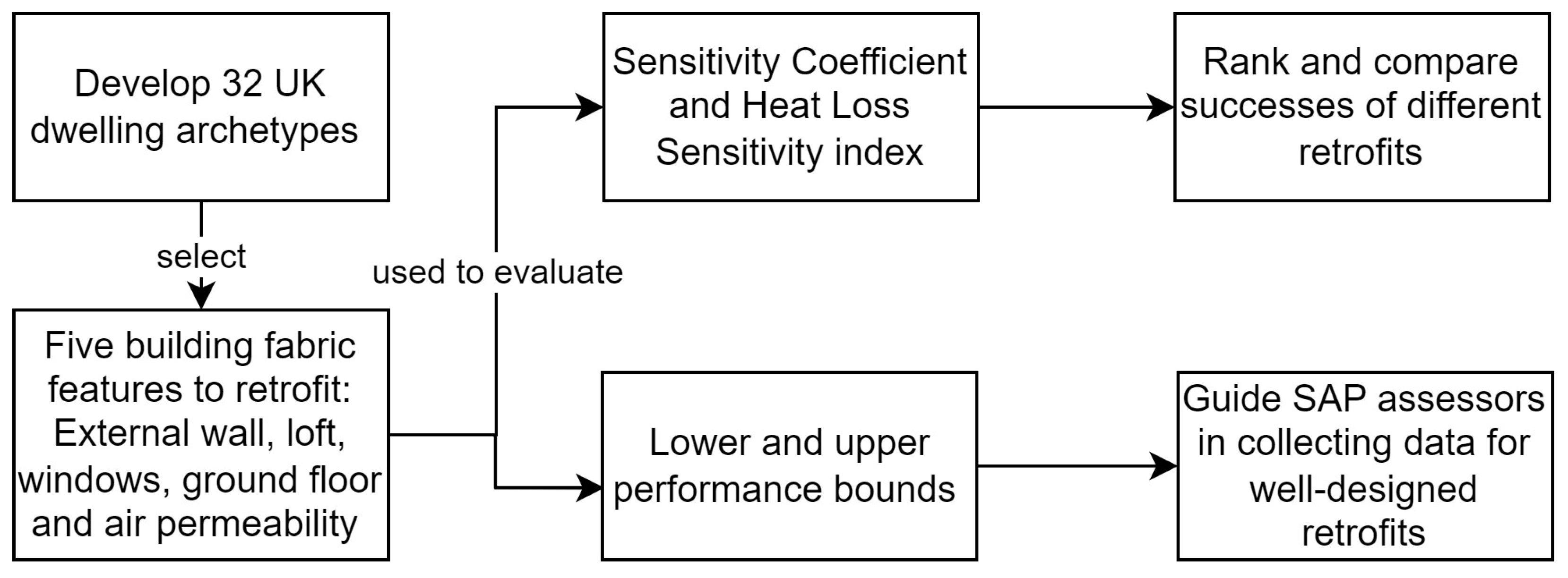
2.1. Overview

The methodology used in this study is summarised in Figure 1. To begin, 32 DTS archetype models were developed to determine the heat loss (in kWh/year) attributable to each of the five main building fabric features: external wall, loft, window, ground floor, and air permeability. Afterwards, a Sensitivity Coefficient (SC) was calculated for each archetype’s building fabric feature by running multiple simulation tests. The SC quantifies the variation in heating energy demand across a specific fabric element when the thermal performance is altered. To determine which building fabric measure to retrofit for each archetype, a metric Heat Loss Sensitivity (HLS) index was created. The HLS index quantifies which fabric makes the biggest difference to whole house energy use when it is improved. Then, each building fabric feature was modified to an upper and lower bound, respectively, and the space heating energy demand was predicted. To further the analysis, the above-mentioned process was repeated with dwellings with different scenarios, for climate, window-to-wall ratio (WWR), and overshadowing.

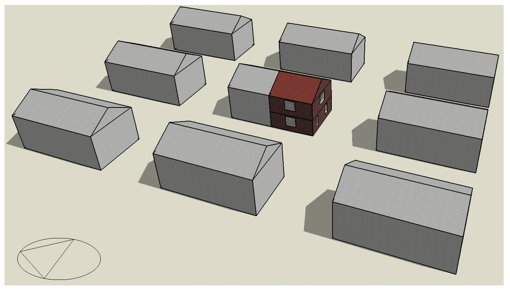
2.2. Development of DTS Archetype Models

DesignBuilder, incorporating EnergyPlus as its physics engine, was used to develop the DTS models. The models use Typical Meteorological Year (TMY) for Leeds [36]. SAP benchmarked climate data in the UK to 21 regions and Leeds (belonging to East Pennines); other regions are also tested and discussed in Section 2.5. Macro-level model inputs (floor area and the number of bedrooms) were taken from the BRE report “ECO3 Deemed Scores Methodology”, which was previously used as a proxy to represent the UK housing stock [35]. Accordingly, 32 building archetypes were developed, made up of nine house types (mid-terrace house, end-terrace house, semi-detached house, detached house, semi-detached/end-terrace bungalow, mid-terrace bungalow, detached bungalow, one-storey flat, and multi-storey flat) and different numbers of bedrooms (one to five). The deemed score methodology used the average geometric characteristics of all dwellings in the UK housing stock to calculate the type and size of archetype dwellings. Whilst the UK housing stock is heterogenous in nature, these approximations provide reasonable estimates of savings for indicative dwellings of each archetype within the stock (Table 1).
The layout of the DTS archetype models is presented in Figure 2. This study assumed that houses have two stories with a pitched roof and bungalows have one storey with a pitched roof. Furthermore, it was assumed that houses and bungalows always had an unoccupied roof and the flats are located on the middle floor.
All archetypes are built pre-1949 (SAP age band A to C) and have the same construction; the construction details are summarised in Table 2. All party walls, floors, and ceilings where there are neighbouring dwellings are treated as adiabatic, as it is assumed that occupancy patterns will be similar to the archetypes, and there is no conductive heat exchange through party walls. The party wall of end-terrace and semi-detached houses is designed to face north, reducing the difference in solar gain. This assumes that all external walls have the same WWR, which makes the impact of orientation less significant. The occupancy patterns and internal heat gain schedules were specified using the National Calculation Method (NCM), which defines model inputs for regulatory compliance calculation in the UK for non-domestic buildings; it does, however, include schedules for domestic spaces, as these can be included in large mixed-use buildings [37]. In addition, linear thermal bridges at junctions were considered; the values are based on SAP Appendix K values in lieu of any available defaults for legacy solid-wall dwellings. Also, the floor-to-ceiling height was assumed to be 2.5 m, which was the average from other field studies [38], and a WWR of 15% was assumed; this aligns with those calculated following SAP conventions and findings from field studies [38].
Zoning was performed according to the SAP, where the living area fraction is calculated by taking into consideration the number of habitable rooms. For instance, a three-bedroom semi-detached house with five total inhabitable rooms (kitchen, lounge, and three bedrooms) would yield a living area fraction value of 0.3. The total floor area for this archetype is 89.2 m2, with 18.7 m2 allocated to the lounge area. The ground floor has been separated into two zones—a lounge (18.7 m2) and a kitchen (25.9 m2). Further, the first floor was assumed to be a single zone with three bedrooms and a bathroom totalling 44.6 m2 in size.
For the lounge, the heating set-point was assumed to be 21 °C. For the kitchen, bedroom, and bathroom, SAP’s equation was employed to calculate the heating set-point, which is 21–0.5*HLP (Heat Loss Parameter). Previous field studies identified that this parameter ranges between 2 to 4 [38]; thus, an average value of 3 was assumed, resulting in a set-point temperature of 19.5 °C. Occupancy and internal heat gains from lighting and equipment were determined using SAP calculations. For instance, a three-bedroom semi-detached house had the equivalent occupant heat gain of 2.69 people, as well as 4.45 W/m2 of internal heat gain in the living room and bedroom areas, with 10.98 W/m2 found in the kitchen area specifically.
The ground temperature in DesignBuilder is assumed to be 18 °C as default for large non-domestic buildings. However, the ground temperature underneath dwellings is different from large non-domestic buildings, and can be considered to be somewhere between the undisturbed ground temperature and the average internal temperature of the dwelling [36]. Thus, the monthly ground temperature was calculated by calculating the monthly average of the undisturbed ground temperature for the UK using MIDAS data from the Met Office for over 100 UK sites [39]. The monthly average under-dwelling ground temperature was then calculated by taking an average of the mean undisturbed ground temperature and internal dwelling temperature. The average internal temperature is taken from a model following heating schedules designed to mimic those cited in SAP, albeit at an hourly resolution.
Table 2. Summary of modelling assumptions of the deemed score archetype DTS models.
Building ElementValueJustification
External wallU-value = 1.7 W/m2KSolid brick wall with thickness < 330 mm [40]
RoofU-value = 2.3 W/m2KSlates or tiles without insulation at joist [41]
LoftU-value = 0.527 W/m2K12.5 mm plasterboard internally + 100 mm mineral wool, assuming the repeat bridging from the wooden joists was 30% of the area
WindowU-value = 2.8 W/m2K, g-value = 0.76Double-glazed unit with a 12 mm PVC frame [41]
Ground floorU-value = 1.2 W/m2KSuspended timber floor without insulation [41].
Air permeabilityAir Permeability rate = 12 m3/hm2@50 PaAverage for dwellings built prior to 1920 according to BRE database of air leakage rate in UK dwellings [42]
Natural ventilation rateVentilation rate = 2 ach−1 when >24 °CNational Calculation Methodology (NCM) [37]
Heating set-pointKitchen, Bathroom and bedroom (19.5 °C), Lounge (21 °C)SAP [41]
Heat gainsVaries according to archetypeSAP [41]
Lighting heat gain4.6 W/m2 lux, assume 300 lux with controlsNCM [37]

2.3. Development of a Metric to Evaluate Fabric Sensitivity

Differential sensitivity analysis was carried out to assess the impact of variations arising from modelling assumptions. It is widely used, as it directly investigates the changes that different input variables will have upon the output variables. Repeated simulations are performed by changing a different input variable each time to determine the individual effects of all the input changes (Equation (1)):
P i = P i P B ,
where P i is the predicted output using modified value of input i, P B is the predicted output using base-case inputs, and ∆Pi refers to the individual effect of each input variation.
The Sensitivity Coefficient (SC) can be determined from the slope of the straight regression line for the data. If more perturbations are used in the analysis for each input variable, a more accurate estimate of the SC can be obtained because there are more data points to calculate the regression line. The correlation between the output and input variable is predicted, as the sensitivity will vary from point to point if not a linear function. To determine the slope of the regression line, the SC shows how sensitive the investigated building fabric is to the change. The SC is a dimensionless value, and its calculation is illustrated in Equation (2):
S C = O P / O P B I P / I P B
where SC is the Sensitivity Coefficient; ΔIP, ΔOP are the changes in input and output; IPB is the base case of input; and OPB is the base case of the corresponding output.
To calculate the SC, five perturbations were tested, as shown in Table 3. The input parameters were varied along with the baseline input, representing a range of possible values for each parameter in the baseline pre-retrofit dwellings. Note that the selected perturbations utilised in the sensitivity analysis can have varied magnitudes, but with no impact on the sensitivity coefficient. To illustrate, this investigation chooses five perturbations for external wall U-values, ranging from 1.3 to 2.1 W/m2K, to calculate the SC. Nonetheless, if a wider range of perturbations were tested, such as the external wall U-values of 0.9 to 2.5 W/m2K, the SC would remain identical. The corresponding output is the space heating energy demand. For each of the five building fabric features, the slope of the regression straight line (ΔOPIP) was obtained from the perturbations, and the SC can be predicted by inputting the respective base case values. Thus, a total of 160 simulations were performed to obtain the SC for each of the 32 archetypes. Based on prior research [31,32,33,34], a linear relationship was expected, fitting between the lower and upper bounds outlined in this study. Should these perturbations reveal non-linearity, they will be revisited in the results section, i.e., more perturbation may need to be evaluated.
Annual heat loss (in kWh per year) through the external wall, roof, windows, ground floor, and via air permeability were outputted from DesignBuilder for each archetype. The annual heat loss was calculated by adding the totals of the hourly heat loss from DTS models. For example, the annual heat loss through the external wall was outputted by the sum of the heat loss to all the zones (kitchen, lounge, bedrooms, and bathroom) from external wall inner surfaces. As a benchmark, Energy Saving Trust suggests the following percentages of heat loss: walls (33%), roof (26%), windows (18%), ventilation and draughts (12%), floors (8%), and doors (3%).
This study proposes a Heat Loss Sensitivity (HLS) index, which is the product of the annual heat loss and SC, used to rank the importance of different building fabric features in retrofit design for each building archetype. It is expressed in units of kWh, and it is important to note that a higher number means that the parameter being ranked is more crucial to take into consideration during retrofit. Note that DesignBuilder simulations are commonly used by engineers to assess the annual heat loss of building fabrics and identify areas for energy efficiency improvements. However, variations in sensitivity to retrofitting mean that using annual heat loss alone is insufficient, underscoring the need for tools like the HLS index.
The HLS percentage metric is derived from the HLS index of various building fabric features to ensure a fair comparison among different archetypes. This approach maintains the consideration of proportionality rather than absolute values. To illustrate, the HLS index of each building fabric feature is combined to calculate the total HLS index. The individual proportions for each feature are then calculated by dividing the HLS index of the feature by the total HLS index, and then expressing this ratio as a percentage. It is crucial to remember that the HLS index’s absolute values can differ significantly based on the size of the building. Thus, for a more accurate evaluation across different building archetypes, the HLS percentages are employed instead of the HLS index.

2.4. Development of Lower and Upper Bound Inputs

Solid-wall dwellings constructed pre-1949 have different building fabric features, which cause a variation of input parameters; this variation can cause an error in the predicted output (space heating energy demand) and, thus, affects the selection of the best retrofit measures. Therefore, a lower bound (the smallest possible input for the building fabric feature) and an upper bound (the largest possible input for the building fabric feature) are defined for the purpose of this work and are summarised in Table 3. The lower and upper bounds presented in this study present the maximum potential range of space heating energy demand variations related to different building fabric features according to the data collected. It should be noted that this study does not account for the distribution of building fabric features falling within this range; instead it is assumed to be uniform. The following describe the performance range for each feature, and the justification for the range selected:
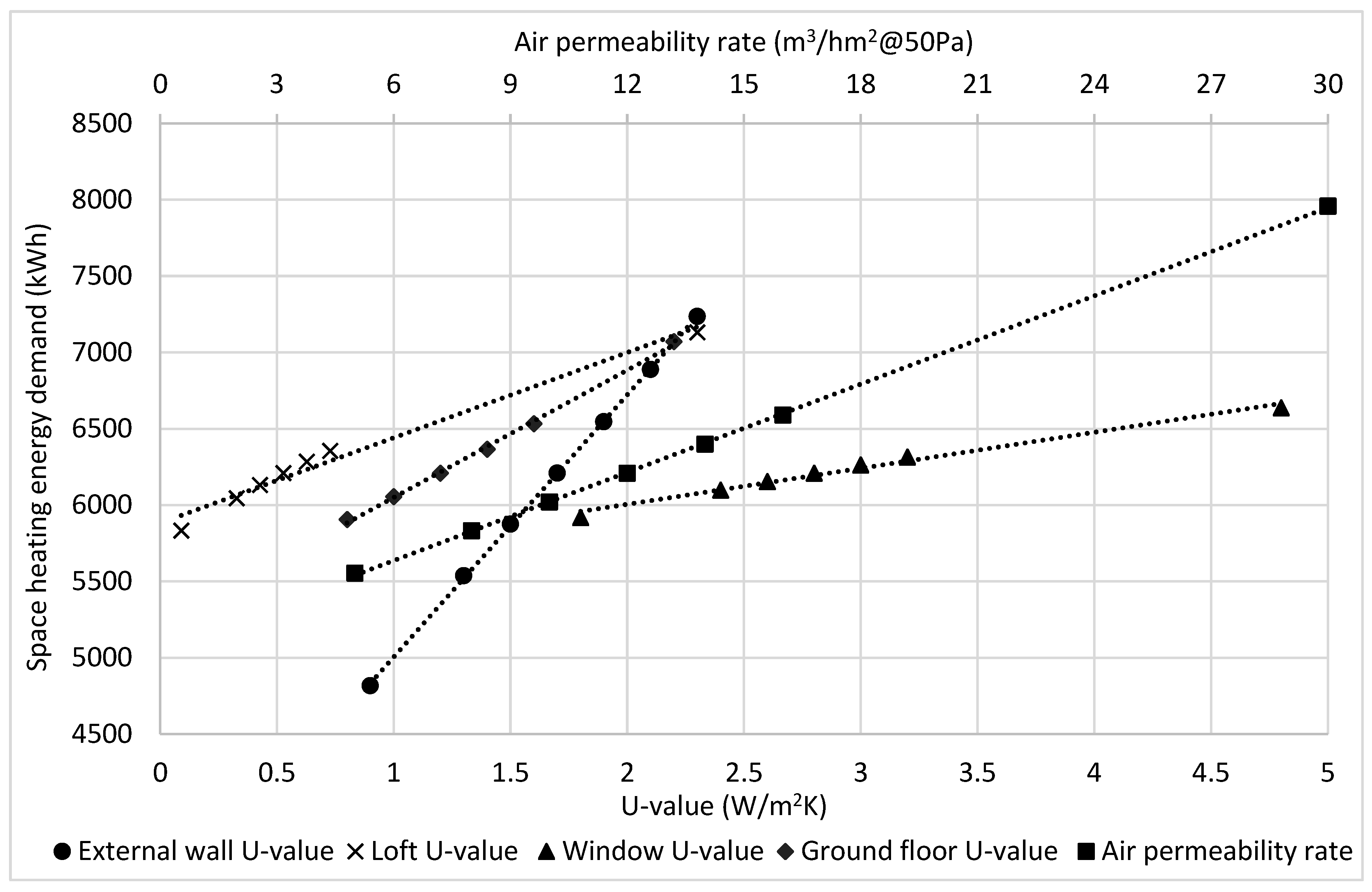
  • U-value of external wall: Hulme and Doran (2015) measured the U-value for standard solid walls (solid brick walls with thickness < 330 mm) for 85 UK dwellings built before 1967; the range of the U-values found was 0.9 to 2.3 W/m2K [40];
  • U-value of loft: A pre-retrofit UK dwelling can have no mineral wool insulation or up to 400 mm mineral wool insulation. Thus, the U-value of a loft is 2.3 W/m2K without mineral wool insulation, and a U-value of 0.09 W/m2K with 400 mm mineral wool insulation was selected [41];
  • U-value of window: SAP (2012) suggested the U-value of 1.8 W/m2K for triple-glazed windows and 4.8 W/m2K for single-glazed windows [41]. As per SAP, the U-value for a double-glazed window varies from 2.0 to 3.1 W/m2K. Therefore, it is not considered in the analysis of lower and upper bounds for scenario evaluation;
  • U-value of ground floor: Pre-retrofit solid-wall dwellings have suspended timber floors. Typically, pre-retrofit UK dwellings have no ground floor insulation, so the lower outlier is selected to be the same as the base case (1.2 W/m2K) installed. However, measurements from field studies suggested that the ground floor U-value can be much higher than 1.2 W/m2K, with 2.2 W/m2K obtained from a field study [38], which was used for the upper bound in this study;
  • Air permeability rate: Stephen (2000) reported the air permeability of 384 UK dwellings using the blower door test, which revealed the range of air permeability to be 5 to 30 m3/m2h@50 Pa [42].
One building fabric feature was varied at a time between the higher and lower bounds, while keeping all other parameters at the base case values. For each fabric element, the percentage change of space heating energy demand due to these outliers was predicted, with a total of 320 simulations. If the absolute percentage change is the highest, it means that having an accurate input for these elements in a pre-retrofit model is more important, and they are ranked accordingly.

2.5. Development of Parameters Impacting Retrofit Performance

The results discussed in the prior section only apply to specific conditions. If the analysis in Section 2.3 and Section 2.4 above is repeated under different conditions, a more comprehensive understanding of how various factors influence the outcome can be obtained. Thus, this study investigates different climates, WWRs, and overshadowing. These variables were chosen based on their proven significant impact on building energy performance, as determined by prior research and theoretical considerations [31,32,34,43,44,45]. This information can then be used to determine where retrofit priorities should lie and to identify the important building fabric features to obtain under different conditions. After simulating the fabric sensitivity and outliers for all 32 building archetypes, a few representative ones are selected for the parametric study to reduce the number of simulations. To illustrate the parametric study process, a three-bedroom semi-detached house archetype was used as an example, as according to the literature, the average number of bedrooms in the UK is 2.95 [46,47].
To evaluate a parameter, all other parameters were kept the same and only one was changed at a time to see its effect on the results. For each parameter, the predicted HLS percentages were compared with the corresponding base case values. The effect that changing the results for a single parameter had on the findings was recorded.

2.5.1. Parameter 1: Climates

SAP benchmarked climate data in the UK to 21 regions [41], as the baseline climate region was set as Leeds (region: East Pennies), which was the UK average. Thus, two locations at opposite ends of the spectrum were tested, London (region: Thames), which has the highest average temperature, and Edinburgh (region: East Scotland), with the lowest temperature. The CIBSE TRY weather file was selected.

2.5.2. Parameter 2: Window-to-Wall Ratios (WWR)

Previous studies on modelling archetype homes in the UK shows that changing the WWR changes the energy saved from wall insulation linearly [45]. The baseline WWR was set at 15%, which is the average of all evidence collected from field studies [38]. In these studies, the WWR ranged from 10% to 25%. Therefore, both the lower limit (10%) and upper limit (25%) were tested.

2.5.3. Parameter 3: Overshadowing

The surrounding buildings located around the archetype dwelling are set back at 9 m to allow space for roads, and they are also assumed to have the same height (Figure 3). It is worth noting that the models in this study show two extremes, with no urban shading (baseline model) and urban shading on all sides (variation), respectively. With that said, real values will fall somewhere between those two extremes [44].

3. Results

The three-bedroom semi-detached home serves as an exemplar to illustrate the findings from this research, as it is one of the most representative archetypes which represents a significant portion of the UK housing stock. The baseline space heating energy demand for a three-bedroom semi-detached house archetype was predicted to be 6210 kWh.

3.1. Sensitivity Coefficient

The space heating energy demand for the five perturbations and two (lower and higher) outliers are shown in Figure 4. The R2 for all the five building fabric features are larger than 0.95 and they are linear; thus, they can be used for differential sensitivity analysis. All other archetypes were also tested, and the results show that the R² for all the five building fabric features is larger than 0.95. Thus, these perturbations reveal a linear relationship, as expected according to Section 2.3. Figure 4 demonstrates that the slope (ΔOPIP) of each building fabric feature can be used to measure how much a change in an input parameter (e.g., external wall) will affect the output parameter (space heating energy demand). For instance, the slope of the external wall is 1717 (y = 1717x + 3287), which is higher than the one for loft at 558. This means that when changes are made to the external wall, it will have a larger impact on the space heating energy demand than changes made to the loft. Figure 4 also indicates that significant variation in space heating energy demands can be observed based on the uncertainty range selected, regardless of the magnitude of their respective slopes. For instance, while the ground floor had a steeper slope (833) than the loft (558), the uncertainty range for space heating energy demand associated with the loft was larger, at 1300 kWh, than that for the ground floor, which had an uncertainty range discrepancy of 860 kWh.
A DesignBuilder simulation outputted the annual heat loss of a building fabric, which can help identify and target any areas that are contributing significantly to its overall energy demand. Typically, engineers use these methods to assess how influential a building fabric is. In this case, the external wall had the highest heat loss of 5346 kWh, followed by windows (3539 kWh), while loft insulation constituted the least amount, at 627 kWh (Figure 5a). When assessing the importance of different building fabric features for energy efficiency improvements, it is important to consider more than just annual heat loss. While some elements may experience a large reduction in space heating energy demand with minor alterations, others may remain unaffected by major modifications. Therefore, it is important to factor in the fabric sensitivities when making such comparisons. One method of comparison which has been utilised is the slope analysis depicted in Figure 4; however, this metric does not take into account discrepancies between the scales and units of various input parameters. For instance, the slope of the air permeability rate (96) appears much smaller than the slope of the loft (558), implying that air permeability is less sensitive. In order to allow for a more meaningful comparison between parameters of different scales and units, the concept of SC was proposed. It normalises changes in inputs and outputs relative to their respective baselines, thus allowing for a closer evaluation of their proportional impacts on each other’s outcomes. Analysis of the sensitivity coefficients presented in Figure 5b indicates that the external wall rated most highly at 0.46, followed by the air permeability rate at 0.18, while the loft had the lowest coefficient at 0.065.

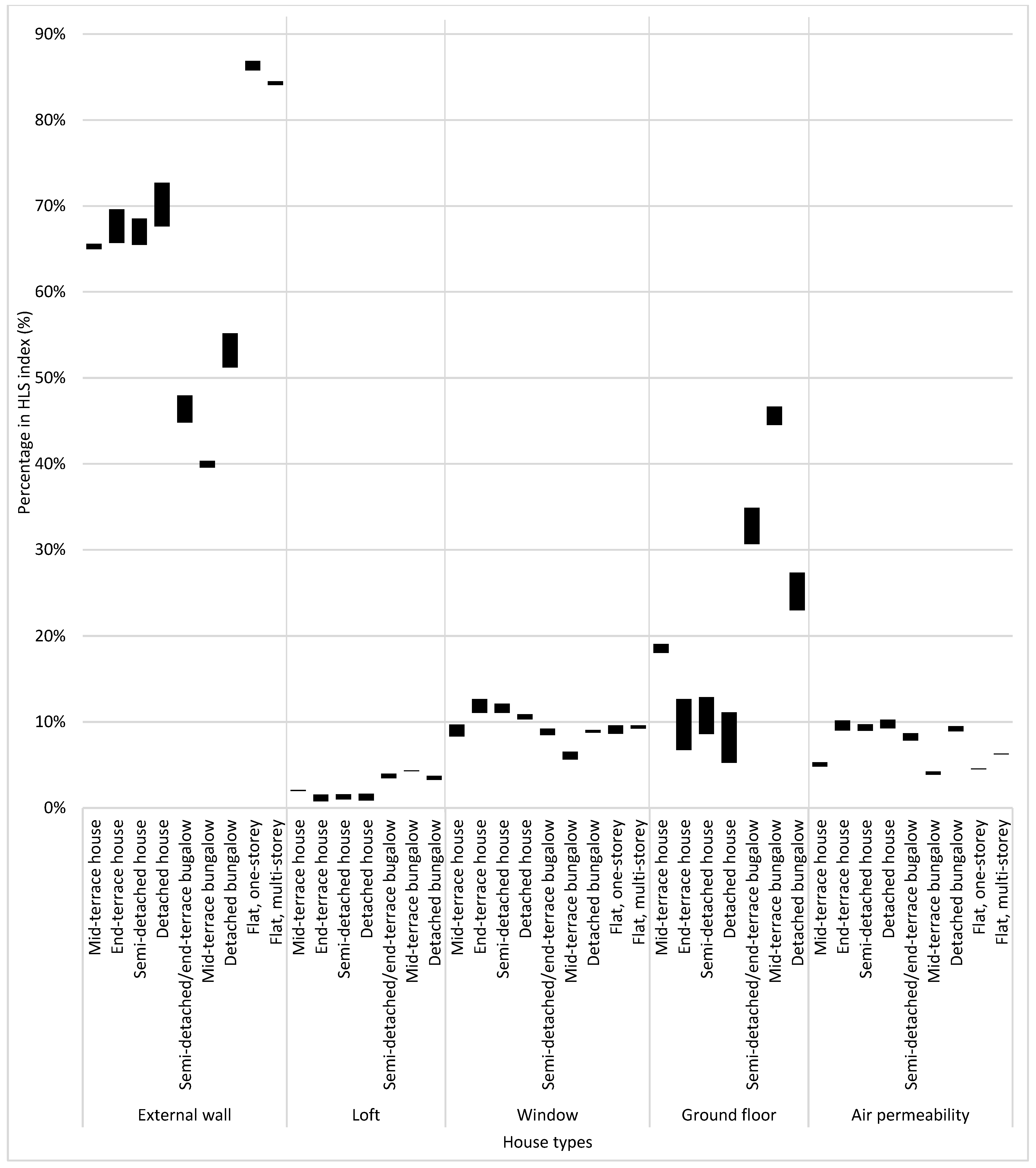
3.2. Heat Loss Sensitivity (HLS) Index and Lower and Upper Bounds

In this study, a novel index (HLS index) has been proposed by calculating the product of the annual heat loss and SC of building fabric features. This index is highly instrumental in determining which elements are most suitable for energy efficiency improvements. The external wall of a building is one of the most important parameters to consider when retrofitting, as it has a high SC and annual heat loss. On the other hand, windows have low SCs, but high annual heat losses. This suggests that while windows are significant contributors to the total thermal energy lost from buildings, reducing the U-value by large amounts may not significantly impact window heat losses. The HLS index from Figure 5c revealed that the external wall was the most critical aspect for retrofitting (2464 kWh), while all other fabric elements performed similarly: windows could reduce space heating demand by 433 kWh, lofts by 41 kWh, ground floors by 348 kWh, and air permeability rate by 345 kWh.
Along with the HLS index, it is necessary to consider lower and upper bounds, as these indicate the range of potential values for building fabric features and the variability of their influence over energy performance. This study shows the maximum possible variation of space heating energy demand for lower and upper bounds for different building fabric features (Figure 6). However, it does not consider the likelihood of a building fabric feature falling within this range, but simply assumes that it is equally probable between the two bounds. As illustrated in Figure 6, the uncertainty of building fabric features has a notable effect on space heating energy demand. The external wall U-value was modelled to have a lower bound of 0.9 W/m2K and an upper bound of 2.3 W/m2K, with the baseline case of 1.7 W/m2K. The lower bound resulted in a space heating energy demand of 4817 kWh, indicating a 1392 kWh (22.4%) change as compared to the base case, whereas the upper bound increased this figure to 7236 kWh, resulting in a 1026 kWh (16.5%) increase compared to the baseline. The results show that the external wall U-value has the largest uncertainty regarding energy demand in a three-bedroom semi-detached house, with a variation ranging from −1392 to 1026 kWh (−22.4% to 16.5%). This is followed by air permeability rate, which has a variation of −655 to 1748 kWh/m2 (−10.6% to 28.2%).

3.3. Fabric Sensitivity and Uncertainty Analysis: A Comparison of Dwelling Types

3.3.1. Space Heating Energy Demand

In an effort to establish a fair comparison, the space heating energy demand per square meter was utilised to examine the variance across different archetypes, considering the diverse number of bedrooms in each case (Figure 7).
A comparison between mid-terrace and end-terrace/semi-detached houses reveals a lower space heating energy demand for the former. This can be attributed to the additional party wall in mid-terrace houses, resulting in reduced external wall heat loss and, consequentially, a lesser heating energy demand. Interestingly, the data do not indicate a significant disparity in the space heating energy demand per square meter between detached and end-terrace/semi-detached houses. A similar pattern is observed in the case of bungalows. The lowest space heating energy demand is in flats, and multi-storey flats exhibit a slightly increased space heating energy demand. The reason may be because the baseline for this investigation was middle-floor flats, which are the most common flat type. In these flats, the ceiling and ground floor are assumed to be adiabatic, which contrasts with mid-terrace houses where there is heat transfer through the loft.

3.3.2. Significance of Fabric Sensitivity on Model Accuracy

In the retrofitting process, Figure 8 serves as a pivotal resource, specifically beneficial for property owners and landlords. This figure highlights the impact of fabric sensitivity on model precision, thereby ranking the relevance of different retrofit interventions. This data can serve as an initial reference point in the decision-making trajectory for retrofit design, thus endorsing a systematic and strategic methodology for enhancing energy efficiency in the UK’s domestic stock.
To ensure a fair comparison, it is imperative to evaluate the HLS index using percentages instead of absolute values across different archetypes. For instance, the three-bedroom semi-detached house illustrated demonstrates an absolute HLS index of 2464 for the external wall, 41 for the loft, 433 for the window, 348 for the ground floor, and 345 for air permeability. When we add up these values, the total HLS index comes out to be 3632. This corresponds to proportions of 67.8%, 1.1%, 11.9%, 9.6%, and 9.5%, respectively. It is important to note that the HLS index’s absolute values vary depending on the size of the building. For example, a six-bedroom detached house may have a higher HLS index compared to a two-bedroom house. However, comparing percentages, rather than absolute values, gives a more precise evaluation when examining different building archetypes. As shown, both the six-bedroom and two-bedroom houses have external wall HLS percentages of 67.6% and 72.1%, respectively, despite the absolute HLS index being 6833 kWh and 3640 kWh (Figure 8).
The findings of this study emphasised the significance of external walls in the retrofitting process for most building types. The only exception to this trend was observed in mid-terrace bungalows, where ground floor emerged as the most crucial factor. In contrast, the loft was considered the least influential factor for retrofitting, except in mid-terrace bungalows where air permeability is the least important. Loft insulation being the least significant factor is potentially due to its existing insulation. Adding more insulation does not significantly reduce the HLS percentage compared to retrofitting other building fabric elements.
The variation in HLS percentage caused by the number of bedrooms significantly impacts both the external walls and the ground floor HLS percentage. In larger houses with more bedrooms, the ground floor becomes more crucial due to a higher percentage of heat loss in relation to the total heat loss of the entire house. However, it is important to note that the number of bedrooms does not shift the primary parameter for retrofitting, which remains the external walls for most archetypes.
Moving on to the comparison between houses and bungalows, there were variations in the HLS percentage between the external walls, loft, and ground floor. Houses exhibited a higher HLS percentage for the external wall, while bungalows demonstrated a higher HLS percentage for the ground floor and loft. The difference can be explained by the architectural design. Bungalows have a higher proportion of the ground floor and loft area contributing to heat loss compared to houses. On the other hand, houses exhibit a higher percentage of heat loss area in their external walls compared to bungalows.
Mid-terrace houses exhibited a lower HLS percentage for external walls and a higher HLS percentage for ground floors. This pattern was consistent when comparing mid-terrace bungalows with other bungalow types, attributable to the additional party wall in mid-terrace structures compared to end-terrace or semi-detached houses. Interestingly, the HLS percentage for external walls and ground floors in detached, semi-detached, and end-terrace houses showed similar results. This pattern also applied to bungalow types. It is worth noting that this equivalence remained consistent despite the distinct architectural feature of detached houses and bungalows, where all four walls are externally facing.
Lastly, regardless of the architectural variances of single-storey and multi-storey flats, they exhibited comparable rankings in terms of the HLS percentage. Notably, retrofitting the external wall holds the highest significance for flats compared to houses and bungalows.

3.3.3. Effect of Lower and Upper Bounds on Fabric Uncertainty

In this research, Figure 9 presents a crucial illustration of how the selected lower and upper bounds in Table 3 affect fabric uncertainty. This visual representation assists in identifying the most influential assumptions to consider in energy models. By adopting this approach, the precision and reliability of fabric retrofit design models for UK domestic stock can be enhanced.
The results of Figure 9 demonstrate that the uncertainty of the building fabric features for each archetype can be calculated by summing the negative and positive bars. For instance, in the case of a three-bedroom semi-detached house, an analysis of varying external wall U-values resulted in a total of +1026 kWh (16.5%) higher and −1392 kWh (22.4%) lower energy consumption demand, respectively, producing a combined uncertainty value of 38.9%. It is important to note that the building fabric feature with the highest uncertainty percentage represents the element that holds the greatest significance for measurement by the SAP assessor, specifically the external wall in this scenario.
Moving on to the fabric uncertainty rankings, they yielded consistent results across different types of houses with varying numbers of bedrooms, albeit with a few exceptions, as shown in Figure 9. For instance, in the case of one-bedroom end-terrace houses, the uncertainty in external wall composition (39.5%) was slightly lower than the air permeability rate (40.1%). Conversely, in three-bedroom houses, the uncertainty in external wall composition (39.0%) was slightly higher than the air permeability rate (38.8%). It is important to note, however, that the number of bedrooms did not significantly affect the level of fabric uncertainty.
Upon detailed examination of distinct housing types, interesting variations are observed. This is particularly contrasting to the HLS index, where external walls emerge as the most crucial parameter to retrofit across most archetypes. For mid-terrace houses, the measurement of external walls takes precedence. However, for semi-detached and end-terrace houses, as well as detached houses, both external wall measurements and air permeability become equally significant. In the case of semi-detached and end-terrace bungalows, the measurements of air permeability and the loft are equally relevant. For detached bungalows, air permeability becomes the most significant factor, while for mid-terrace bungalows, measuring the loft holds the highest level of importance. Lastly, for flats, the measurement of external walls is the most important.
Finally, when considering the least important parameter, windows emerge as the least significant parameter to measure. Conversely, when considering retrofitting, the loft is deemed the least significant parameter.

3.3.4. Selection of Representative Archetypes

The results of the analysis conducted in this section showed that the number of bedrooms did not significantly affect either the fabric sensitivity or uncertainty rankings. The fabric sensitivity and uncertainty analysis revealed that some house types had similar rankings. Consequently, the dwelling types studied were categorised into five categories: (1) mid-terrace house; (2) end-terrace, semi-detached, and detached house; (3) mid-terrace bungalow; (4) end-terrace/semi-detached and detached bungalow; and (5) one-storey and multi-storey flats. Thus, parametric analysis in the next section will only be carried out for three-bedroom archetypes, which is representative of the average UK home size of 88 m2 reported in the 2001 English House Condition Survey [46].

3.4. Evaluation of Parameters Impacting Retrofit Performance

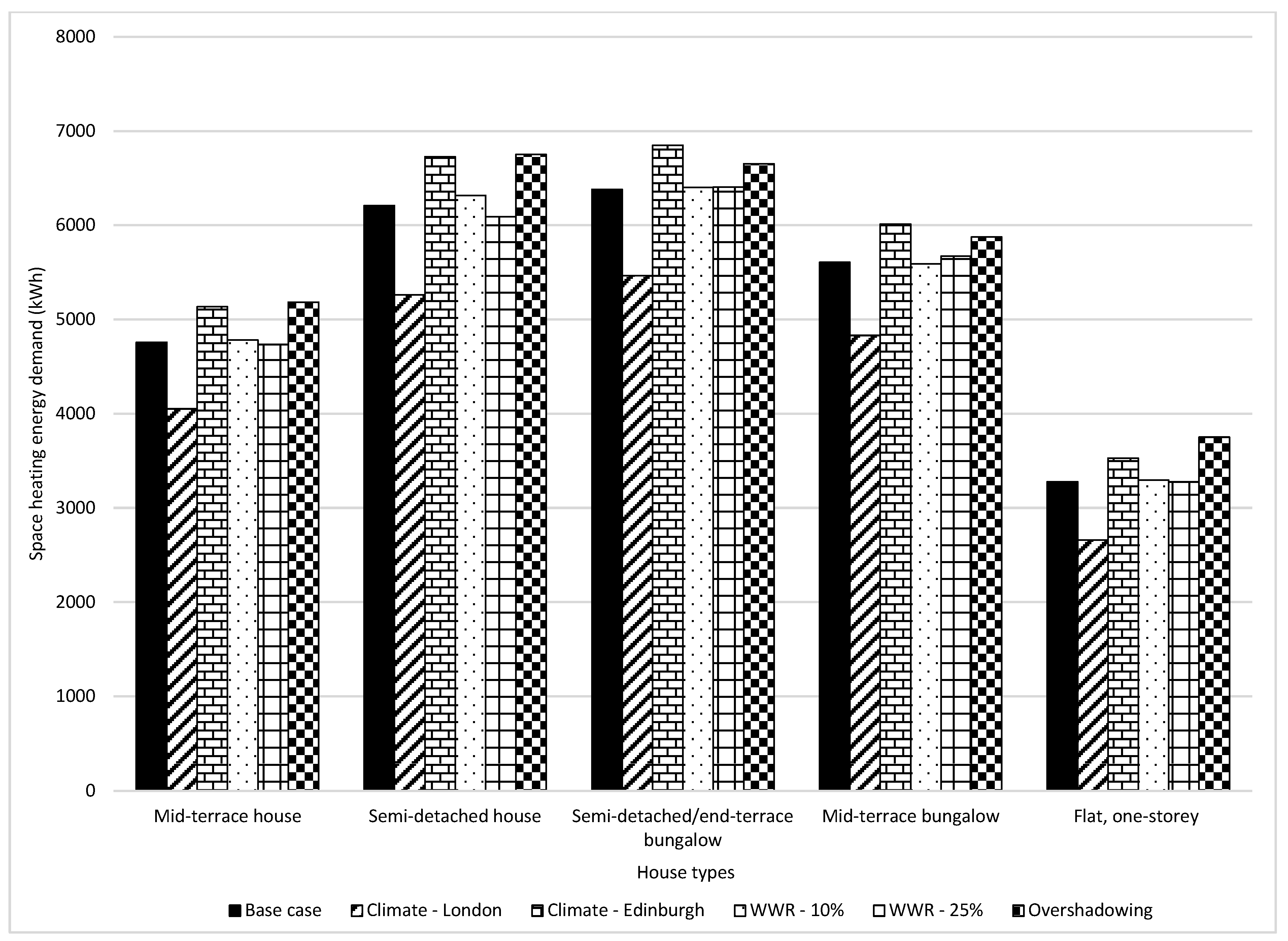
3.4.1. Impact on Space Heating Energy Demand

Figure 10 demonstrates how different parameters impact space heating energy demand. These parameters, thoroughly discussed in Section 2.5, were chosen because previous research has shown their substantial influence on building energy performance. This section further elaborates on the impact of these parameter adjustments on space heating energy demand:
  • Climates: The climate in London, which is warmer than Leeds, results in a decrease in space heating energy demand, ranging from 13.8–18.8%. Conversely, Edinburgh’s climate, colder than Leeds, necessitates a higher space heating energy demand, ranging from 7.3–8.3%.
  • WWRs: Shifting the WWR from 15% to 10% and 25% does not significantly alter the overall space heating energy demand. However, it results in a reordering of retrofit importance, which will be further discussed in subsequent sections.
  • Overshadowing: Overshadowing results in a higher increase in space heating energy demand for houses compared to bungalows. This could be attributed to the larger portions of the house being shaded from solar exposure, necessitating additional heating.

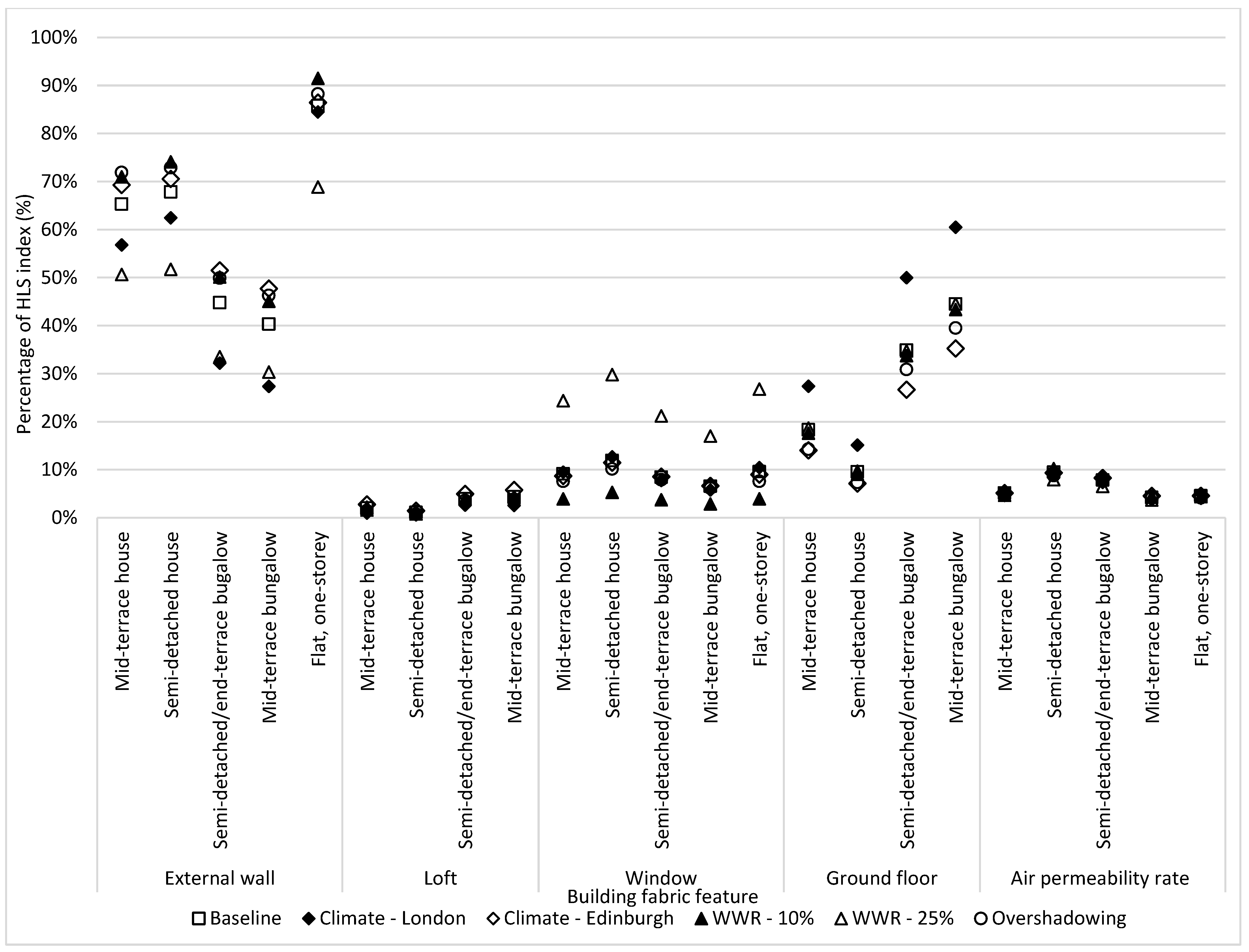
3.4.2. Impact on Heat Loss Sensitivity (HLS) Percentage

When analysing the impact of climates on the HLS percentage, notable differences were observed in the external walls and ground floors (Figure 11). In warmer climates like London, compared to the baseline of Leeds, there was an increase in the HLS percentage attributed to external walls, while the HLS percentage of the ground floor decreased. This observation can be explained by reduced heat loss through external walls in areas with higher temperatures. While the model assumes a constant ground floor temperature across all climates, the importance of ground floor insulation becomes more apparent, leading to an increase in its HLS percentage. Therefore, variations in HLS percentages led to changes in retrofit rankings in London. External wall retrofit remained crucial for houses and flats, while for bungalows, ground floor retrofit became the most critical parameter. On the other hand, when it comes to houses, bungalows, and flats in Edinburgh, the most crucial aspect of retrofitting is the external wall. This is due to the decrease in the HLS percentage of the ground floor and the increase in the HLS percentage of the external wall.
Increasing the WWR results in a higher HLS percentage for windows and a lower HLS percentage for the external wall, while other building fabric features remain constant. Retrofitting the external wall remains the most important for houses and flats, with a 25% WWR. For bungalows, reducing the HLS percentage of the external wall highlights the significance of the ground floor, which already has a high HLS percentage, as the primary parameter for retrofitting.
The introduction of overshadowing had minimal impact on the HLS percentage, thereby not significantly affecting the retrofit rankings. However, a minor increase in the external wall HLS percentage was noted, due to the reduced solar gains in certain shaded areas, leading to a higher heat loss from the external walls.

4. Discussion

The results validate and quantify the intuitive understanding of many professionals (e.g., SAP assessors and retrofit designers). For instance, the external walls play a crucial role in a building’s energy performance. However, it also provides a more nuanced, novel, and evidence-based analysis which can be used to develop guidance for professionals policy makers and householders to optimise retrofit decisions by making them bespoke to a specific home or homes. It also provides some indication of the scale and order of the magnitude of the impact on retrofit performance resulting from varying characteristics found in homes. The following points highlight the implications of each building fabric feature:
  • Solid external walls had the highest SC, HLS index, and impact on space heating demand when likely upper and lower bounds were considered for all archetype homes, regardless of bedroom size (Figure 8), climate, or window-to-wall ratio. They should, therefore, be prioritised in any retrofit projects on solid-walled homes. These findings suggest that the use of a limited default U-value for all solid-walled homes in RdSAP may be particularly problematic, as this is not likely to accurately represent the range in performance and benefits that may be achieved by SWI.
  • Windows had a similar SC to air permeability and ground floors, but had a relatively lower HLS index, though in flats, where the WWRs are larger, the HLS index was higher. The range in likely performance for double-glazing is relatively low and, therefore, upgrading older double-glazing units may not need to be prioritised, unless the home has a particularly high WWR. Upgrading from single- to double-glazed windows should be prioritised in retrofitting.
  • Air permeability had a similar SC to windows and ground floors and a relatively low HLS index. However, despite this, because there can be tremendous variation in air permeability in homes, it could be an important retrofit consideration for some, but not all, homes. For instance, in homes with excessive air leakage, air permeability can exceed external walls in terms of heat loss. Air permeability is, therefore, an important parameter to measure and it may be beneficial to set a requirement to measure air permeability in all homes having retrofit, as well as considering a minimum air permeability threshold for existing dwellings undergoing retrofits. More work would be needed to understand what an acceptable threshold for existing homes may be.
  • Lofts had a similar SC to ground floors and air permeability and a greater SC than windows. However, they had among the lowest HLS indexes, meaning they may not usually need prioritising in retrofitting. Despite this, it is important to inspect the loft condition and existing insulation depths, since loft insulation may not always be to a good standard or even present, and in these cases, lofts become a significant retrofit consideration, especially in bungalows, where they can be as important as walls.
  • Ground floors had a similar SC to lofts and air permeability and a relatively low HLS index in all homes, except bungalows, where the HLS index was higher, indicating that they should be higher retrofit priorities for bungalows. Furthermore, climatic region had a greater influence on ground floor retrofit than other retrofit types, perhaps indicating that ground floor retrofits should be higher priorities in areas of the UK where average annual ground floor temperatures are lower.
The HLS index can be a valuable tool for guiding retrofitting efforts. For example, a high HLS index for the external wall in this study suggests that enhancing wall insulation could lead to significant energy savings. However, it is important to note that while the HLS index indicates the areas of greatest heat loss, it does not necessarily identify the most cost-effective retrofitting opportunities. Decision-making should also consider factors like the cost and feasibility of different retrofitting options. For example, the installation of external wall insulation may not be feasible in certain dwellings due to planning permissions. Therefore, future research could focus on investigating energy savings achievable through retrofitting the building fabric features and calculating the payback period.
However, this research provides useful information that can be used to optimise retrofit decision-making to ensure they are informed by specific features of homes. It also highlights what data are important to capture as part of pre-retrofit surveys, specifically the air tightness level of the home, as well as the condition of the loft insulation and the WWR. Current retrofit policy does not require that the air tightness of homes is measured pre- or post-retrofits to help guide decision-making or set a minimum performance threshold, and EPCs assume a default air permeability rate in homes, not a measured performance. Further EPC assessments are often performed without access to verify loft insulation quality or depth, and they do not require a specific WWR to be captured. These omissions are problematic if EPC functions include informing householders on what retrofit to undertake on their homes.
This study focused on developing and applying the HLS index in the context of retrofitting design for solid-wall dwellings in the UK. While overheating analysis, post-retrofit energy savings evaluation, and informing housing retrofit policies globally were not part of this study, the repeatable methodology and open-source DTS archetype models provided can guide future research in these areas.

5. Conclusions

This research developed a method of retrofit design for UK domestic stock that would enable decision makers to determine which building fabric features should be prioritised to retrofit and assist SAP assessors in their collation of key input data. Through the use of DTS modelling and SC calculations, 32 archetype solid-walled dwellings with different numbers of bedrooms and house types were analysed.
The main findings of this paper can be summarised as follows:
  • External Wall Retrofitting: The HLS index validates professional intuition regarding the significance of external walls in retrofitting due to their high SC and annual heat loss. Policies should prioritise solid-wall insulation as a key retrofit measure.
  • Air Permeability Assessment: Given the wide range of air permeability levels among homes, it is advisable to conduct an air permeability test, such as the Pulse test, before retrofitting. For homes with high air permeability, sealing gaps to improve airtightness could be a more cost-effective solution than implementing EWI, while also reducing carbon emissions.
  • Decision-making Tools: Figure 8 and Figure 9 function as effective decision-making tools, helping prioritise building fabric features for retrofitting and guiding SAP assessors in data collection for well-designed retrofits.
  • Tool Effectiveness across Different Conditions: Parametric simulations showed that climatic regions, WWRs, and overshadowing did not significantly alter the rankings of retrofit features. This confirms the tool’s applicability across diverse UK housing conditions.
In light of these findings, it is clear that tailored solutions, taking into account the specific context, are crucial for retrofitting homes across the diverse architectural landscape of the UK. By adopting this retrofit design approach, there is potential to enhance the reliability of retrofit policies and bridge the gap between predicted and actual performance. Therefore, it is imperative for UK policymakers and SAP assessors to implement this approach when formulating a successful retrofitting plan. This tool is specifically designed for solid-wall homes, but further research could explore its applicability to homes with cavity walls.

Author Contributions

Conceptualization, C.T., J.P. and D.G.; methodology, C.T., J.P. and D.G.; software, C.T. and J.P; validation, J.P. and D.G.; formal analysis, C.T. and J.P.; investigation, C.T., J.P. and D.G.; resources, J.P. and D.G.; data curation, C.T.; writing—original draft preparation, C.T.; writing—review and editing, C.T., J.P. and D.G.; visualization, C.T., J.P. and D.G.; supervision, J.P. and D.G.; project administration, D.G.; funding acquisition, D.G. All authors have read and agreed to the published version of the manuscript.

Funding

This research was part of Demonstration of Energy Efficiency Potential (DEEP) project, funded by Department for Energy Security and Net Zero (DESNZ). DESNZ is a UK ministerial department dedicated to securing long-term energy supply, bringing down bills and halving inflation. The APC was funded by the University of Salford.

Data Availability Statement

Data supporting this study are openly available from University of Salford Repository (USIR) at DOI: 10.17866/rd.salford.25436326.

Conflicts of Interest

The authors declare no conflicts of interest. The funders had no role in the design of the study; in the collection, analyses, or interpretation of data; in the writing of the manuscript; or in the decision to publish the results.

References

  1. HM Goverment. 2019 UK Greenhouse Gas Emissions; Department of Business, Energy and Industrial Strategy: London, UK, 2021. [Google Scholar]
  2. HM Goverment. National Statistics, Energy Consumption in the UK 2021; Department of Business, Energy and Industrial Strategy: London, UK, 2021. [Google Scholar]
  3. HM Government. Policy Paper, The Ten Point Plan for a Green Industrial Revolution; Department of Business, Energy and Industrial Strategy: London, UK, 2020. [Google Scholar]
  4. Kelly, M.J. Retrofitting the existing UK building stock. Build. Res. Inf. 2009, 37, 196–200. [Google Scholar] [CrossRef]
  5. Power, A. Does demolition or refurbishment of old and inefficient homes help to increase our environmental, social and economic viability? Energy Policy 2008, 36, 4487–4501. [Google Scholar] [CrossRef]
  6. Boardman, B. Home Truths: A Low Carbon Strategy to Reduce UK Housing Emissions by 80% by 2050; University of Oxford Environmental Change Institute: Oxford, UK, 2007. [Google Scholar]
  7. Killip, G. Building a Greener Britain: Transforming the UK’s Existing Housing Stock; Environmental Change Institute: Oxford, UK, 2008. [Google Scholar]
  8. HM Government. Live Tables on Dwelling Stock Including Vacants. Table 101: By Tenure, United Kingdom; HM Government: London, UK, 2014. [Google Scholar]
  9. HM Government. Policy Paper, Clean Growth Strategy: Executive Summary; Department of Business, Energy and Industrial Strategy: London, UK, 2018. [Google Scholar]
  10. HM Government. The Climate Change Act 2008 (2050 Target Amendment) Order 2019; The Stationery Office Limited: London, UK, 2019. [Google Scholar]
  11. HM Goverment. Statistical Data Set; Live Tables on Energy Performance of Buildings Certificates, Table D1: Domestic Energy Performance Certificates for All Dwellings by Energy Efficiency Rating; Department of Business, Energy and Industrial Strategy: London, UK, 2021. [Google Scholar]
  12. HM Government. Annual Fuel Poverty Statistics in England, 2021 (2019 Data); Department of Business, Energy and Industrial Strategy: London, UK, 2021. [Google Scholar]
  13. HM Government. Press Release; Government Boosts Energy Efficiency Spending to £1.3 Billion with Extra Funding for Green Homes; Department of Business, Energy and Industrial Strategy: London, UK, 2021. [Google Scholar]
  14. HM Government. Household Energy Efficiency Statistics, Headline Release September 2021; Department of Business, Energy and Industrial Strategy: London, UK, 2021. [Google Scholar]
  15. HM Government. How Heating Controls Affect Domestic Energy Demand: A Rapid Evidence Assessment; Department of Energy & Climate Change: London, UK, 2014. [Google Scholar]
  16. HM Government. National Energy Efficiency Data-Framework (NEED): Summary of Analysis, Great Britain, 2021; Department of Business, Energy and Industrial Strategy: London, UK, 2021. [Google Scholar]
  17. HM Government. The Government’s Standard Assessment Procedure for Energy Rating of Dwellings, 2012nd ed.; DECC, Ed.; Building Research Establishment Ltd: Watford, UK, 2014. [Google Scholar]
  18. HM Government. PAS 2035:2019 Retrofitting Dwellings for Improved Energy Efficiency—Specification and Guidance; BSI Standards Limited 2019: London, UK, 2019. [Google Scholar]
  19. HM Government. Standard Assessment Procedure: Guidance on How Buildings Will Be SAP Energy Assessed under the Green Deal and on Recent Changes to Incentivise Low Carbon Developments; DECC, Ed.; HMSO: London, UK, 2013. [Google Scholar]
  20. Kelly, S.; Crawford-Brown, D.; Pollitt, M.G. Building performance evaluation and certification in the UK: Is SAP fit for purpose? Renew. Sustain. Energy Rev. 2012, 16, 6861–6878. [Google Scholar] [CrossRef]
  21. Zhang, Y.; Zhang, X.; Huang, P.; Sun, Y. Global sensitivity analysis for key parameters identification of net-zero energy buildings for grid interaction optimization. Appl. Energy 2020, 279, 115820. [Google Scholar] [CrossRef]
  22. Silva, A.S.; Ghisi, E. Estimating the sensitivity of design variables in the thermal and energy performance of buildings through a systematic procedure. J. Clean. Prod. 2020, 244, 118753. [Google Scholar] [CrossRef]
  23. Vivian, J.; Chiodarelli, U.; Emmi, G.; Zarrella, A. A sensitivity analysis on the heating and cooling energy flexibility of residential buildings. Sustain. Cities Soc. 2020, 52, 101815. [Google Scholar] [CrossRef]
  24. Mahar, W.A.; Verbeeck, G.; Reiter, S.; Attia, S. Sensitivity Analysis of Passive Design Strategies for Residential Buildings in Cold Semi-Arid Climates. Sustainability 2020, 12, 1091. [Google Scholar] [CrossRef]
  25. Maučec, D.; Premrov, M.; Leskovar, V.Ž. Use of sensitivity analysis for a determination of dominant design parameters affecting energy efficiency of timber buildings in different climates. Energy Sustain. Dev. 2021, 63, 86–102. [Google Scholar] [CrossRef]
  26. Pernetti, R.; Garzia, F.; Filippi Oberegger, U. Sensitivity analysis as support for reliable life cycle cost evaluation applied to eleven nearly zero-energy buildings in Europe. Sustain. Cities Soc. 2021, 74, 103139. [Google Scholar] [CrossRef]
  27. Ebrahimi-Moghadam, A.; Ildarabadi, P.; Aliakbari, K.; Fadaee, F. Sensitivity analysis and multi-objective optimization of energy consumption and thermal comfort by using interior light shelves in residential buildings. Renew. Energy 2020, 159, 736–755. [Google Scholar] [CrossRef]
  28. Prataviera, E.; Vivian, J.; Lombardo, G.; Zarrella, A. Evaluation of the impact of input uncertainty on urban building energy simulations using uncertainty and sensitivity analysis. Appl. Energy 2022, 311, 118691. [Google Scholar] [CrossRef]
  29. Na Tran, L.; Gao, W.; Ge, J. Sensitivity analysis of household factors and energy consumption in residential houses: A multi-dimensional hybrid approach using energy monitoring and modeling. Energy Build. 2021, 239, 110864. [Google Scholar] [CrossRef]
  30. Lomas, K.J.; Eppel, H. Sensitivity analysis techniques for building thermal simulation programs. Energy Build. 1992, 19, 21–44. [Google Scholar] [CrossRef]
  31. Kavgic, M.; Mumovic, D.; Summerfield, A.; Stevanovic, Z.; Ecim-Djuric, O. Uncertainty and modeling energy consumption: Sensitivity analysis for a city-scale domestic energy model. Energy Build. 2013, 60, 1–11. [Google Scholar] [CrossRef]
  32. Cheng, V.; Steemers, K. Modelling domestic energy consumption at district scale: A tool to support national and local energy policies. Environ. Model. Softw. 2011, 26, 1186–1198. [Google Scholar] [CrossRef]
  33. Hughes, M.; Palmer, J.; Cheng, V.; Shipworth, D. Sensitivity and uncertainty analysis of England’s housing energy model. Build. Res. Inf. 2013, 41, 156–167. [Google Scholar] [CrossRef]
  34. Firth, S.K.; Lomas, K.J.; Wright, A.J. Targeting household energy-efficiency measures using sensitivity analysis. Build. Res. Inf. 2010, 38, 24–41. [Google Scholar] [CrossRef]
  35. Hulme, J.; Henderson, J. ECO3 Deemed Scores Methodology; BRE: Watford, UK, 2018. [Google Scholar]
  36. DesignBuilder Software Ltd. DesignBuilder Version 7.0.2.006; DesignBuilder Software Ltd: Stroud, UK, 2022. [Google Scholar]
  37. HM Government. National Calculation Methodology (NCM) Modelling Guide (for Building other than Dwellings in England and Wales); BRE Ltd: London, UK, 2021. [Google Scholar]
  38. Glew, D. Demonstration of Energy Efficiency Potential (DEEP); Technical Report; Department for Energy Security and Net Zero: London, UK, 2024. Available online: https://www.gov.uk/government/publications/demonstration-of-energy-efficiency-potential-deep (accessed on 14 March 2024).
  39. Met Office. Met Office Integrated Data Archive System (MIDAS) Land and Marine Surface Stations Data (1853-Current); NCAS British Atmospheric Data Centre: London, UK, 2012. [Google Scholar]
  40. Hulme, J.; Doran, S. In-Situ Measurements of Wall U-Values in English Housing; BRE: Watford, UK, 2014. [Google Scholar]
  41. BRE. SAP 2012. The Government’s Standard Assessment Procedure for Energy Rating of Dwellings 2012; Building Research Establishment: Watford, UK, 2017. [Google Scholar]
  42. Stephen. BRE Report 359, Airtightness in UK Dwellings: BRE’s Test Results and Their Significance; Building Research Establishment: Watford, UK, 1998. [Google Scholar]
  43. Stone, A.; Shipworth, D.; Biddulph, P.; Oreszczyn, T. Key factors determining the energy rating of existing English houses. Build. Res. Inf. 2014, 42, 725–738. [Google Scholar] [CrossRef]
  44. Parker, J. The Leeds urban heat island and its implications for energy use and thermal comfort. Energy Build. 2021, 235, 110636. [Google Scholar] [CrossRef]
  45. Glew, D.; Parker, J.; Thomas, F.; Hardy, A.; Brooke-Peat, M.; Gorse, C. Thin Internal Wall Insulation (TIWI) Measuring Energy Performance Improvements in Dwellings Using Thin Internal Wall Insulation Annex C; Predicting TIWI Impact Energy & Hygrothermal Simulations; Technical Report; Department of Business, Energy and Industrial Strategy: London, UK, 2021. [Google Scholar]
  46. HM Government. The English House Condition Survey; Department of Communities and Local Government: London, UK, 2007. [Google Scholar]
  47. Statista. Average Number of Bedrooms in Newly-Built Houses in Britain in Each Decade Since the 1930s. Available online: https://www.statista.com/statistics/1056041/average-number-bedrooms-new-british-houses-1930-2020/#:~:text=From%20the%201930s%20until%20the,to%202.95%20rooms%20per%20house (accessed on 14 March 2024).
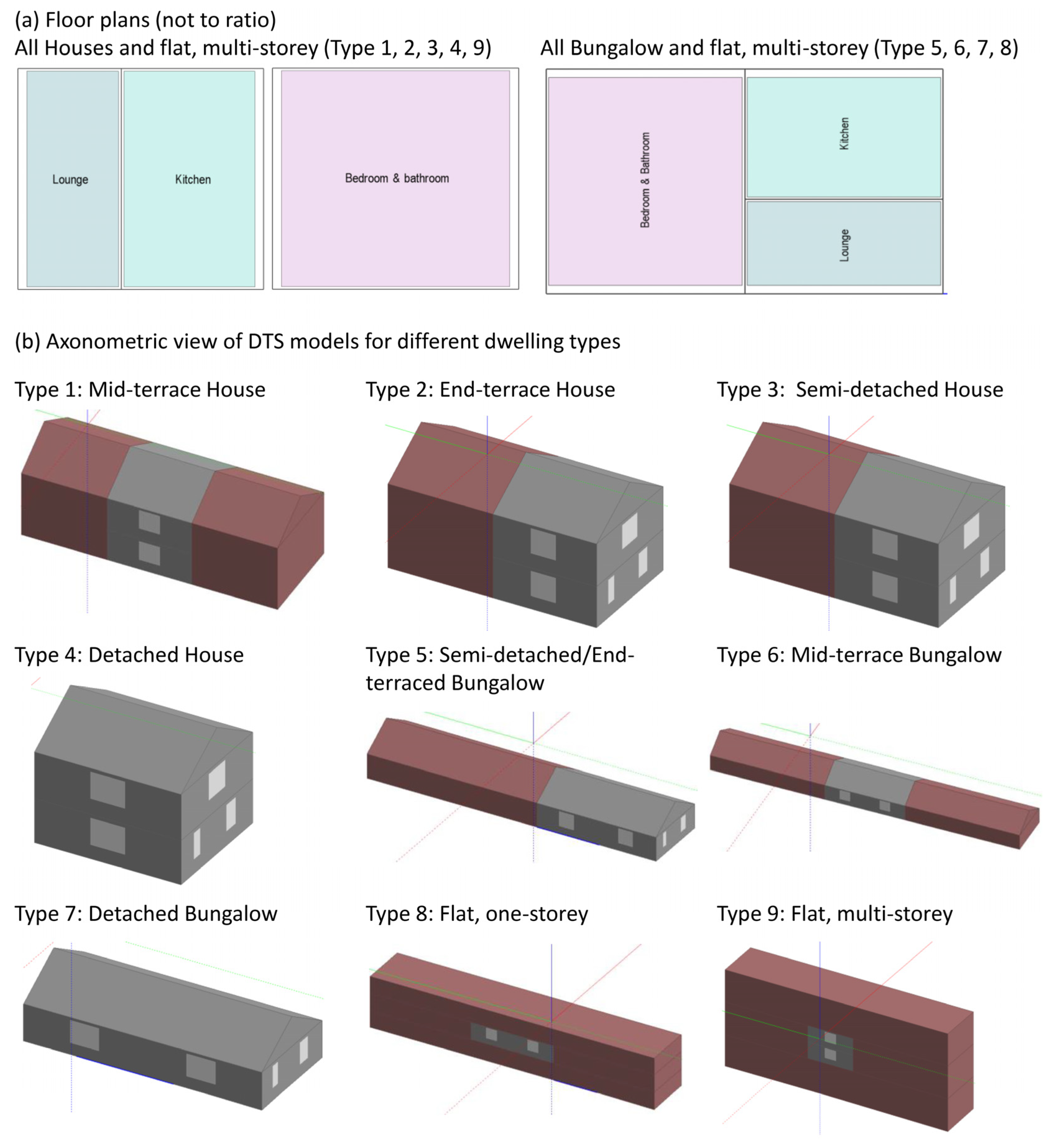
Figure 1. Summary of the methodology used in this study.
Buildings 14 00834 g001
Figure 2. (a) Floor plan and (b) DTS models of three-bedroom building archetype for different dwelling types.
Buildings 14 00834 g002
Figure 3. Model visualisations showing overshadowing from surrounding buildings.
Buildings 14 00834 g003
Figure 4. Space heating energy demand for the five perturbations, and lower and upper bounds (defined in Table 3) for 15% WWR semi-detached three-bedrooms house.
Buildings 14 00834 g004
Figure 5. (a) Annual heat loss, (b) sensitivity coefficient, and (c) heat loss sensitivity index for the five building fabric features.
Buildings 14 00834 g005
Figure 6. Percentage change relative to the base case for combined lower and upper bounds for five building fabric features, with the data labels showing the input parameters (U-values and air permeability) in Table 3.
Buildings 14 00834 g006
Figure 7. Space heating energy demand for different house types; the bar represents data from homes with different numbers of bedrooms (one to four bedrooms).
Buildings 14 00834 g007
Figure 8. Significance of fabric sensitivity on model accuracy for all the 32 dwelling archetypes; the bar represents data from different numbers of bedrooms.
Buildings 14 00834 g008
Figure 9. Effect of selected lower and upper bounds on fabric uncertainty for all the 32 archetypes; the bar represents data from different numbers of bedrooms.
Buildings 14 00834 g009
Figure 10. Variation in space heating energy demand for selected house types when different parameters are alternated compared to the baseline.
Buildings 14 00834 g010
Figure 11. Significance of fabric sensitivity with varying climates, WWRs, and overshadowing compared to baseline.
Buildings 14 00834 g011
Table 1. Characteristics of the 32 dwelling archetypes. Reprinted/adapted with permission from Ref. [35]. 2018, J. Hulme & J. Henderson.
Dwelling TypeNo. of BedroomsMean Total Floor Area (m2)
Type 1: Mid-terrace House151.0
269.4
388.4
4127.8
5180.5
Type 2: End-terrace House151.0
269.4
388.4
4127.8
5180.5
Type 3: Semi-detached House272.5
389.2
4134.6
5191.4
Type 4: Detached House299.7
3115.7
4154.9
5228.7
6320.2
Type 5: Semi-detached or End-terrace Bungalow145.7
258.9
387.1
Type 6: Mid-terrace Bungalow145.7
258.9
387.1
Type 7: Detached Bungalow275.9
3111.9
Type 8: Flat, one storey145.7
265.6
386.5
Type 9: Flat, multi-storey, i.e., maisonettes273.8
3100.7
Table 3. Perturbations and lower and upper bounds of the five building fabric features tested.
Building Fabric FeaturesBaselinePerturbationsLower BoundUpper BoundReference
Solid external wall U-value (W/m2K)1.71.3, 1.5, 1.9, 2.10.92.3[40]
Loft U-value (W/m2K)0.5270.327, 0.427, 0.627, 0.7270.092.3[38]
Window U-value (W/m2K)2.82.4, 2.6, 3.0, 3.21.84.8[38]
Suspended ground floor U-value (W/m2K)1.20.8, 1.0, 1.4, 1.61.22.2[38]
Air permeability rate (m3/hm2@50 Pa)128, 10, 14, 16530[42]
Disclaimer/Publisher’s Note: The statements, opinions and data contained in all publications are solely those of the individual author(s) and contributor(s) and not of MDPI and/or the editor(s). MDPI and/or the editor(s) disclaim responsibility for any injury to people or property resulting from any ideas, methods, instructions or products referred to in the content.

