
Wireless Sensor Placement Optimization for Bridge Health Monitoring: A Critical Review


Abstract
1. Introduction
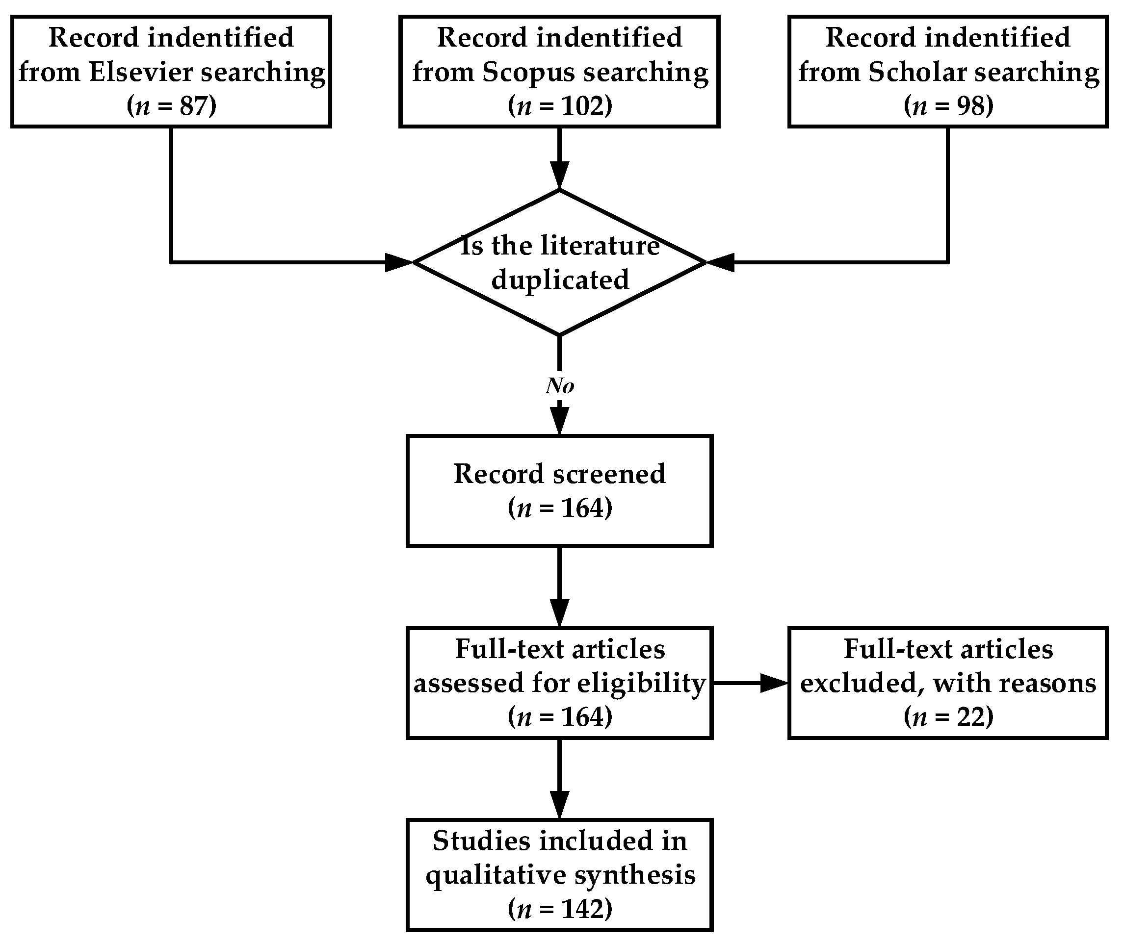
2. Research Methods
3. Sensing Technologies for Bridge Health Monitoring
3.1. Acceleration Sensors
3.2. Global Navigation Satellite System (GNSS)
3.3. Magnetic Sensors
3.4. Strain Sensors
4. Wireless Sensors for Bridge Health Monitoring
4.1. Current Applications
4.2. Data Collection and Transmission
4.2.1. Efficiency
4.2.2. Data Storage
4.2.3. Low Power
4.2.4. Data Quality
4.2.5. Long-Distance Transmission
4.3. Data Processing and Analysis
4.3.1. Data Processing
4.3.2. Data Analysis
4.3.3. Data Aggregation
5. Wireless Sensor Placement Optimization
5.1. Modal Evaluation Criteria
5.2. Wireless Sensor Network Performance Evaluation
5.3. Multi-Objective Optimization Models and Algorithms
5.4. Adverse Environmental Effects
6. Challenges and Future Work
6.1. Efficiency
6.2. Energy Consumption
6.3. Long-Distance Transmission
6.4. An Integrated Layout Solution
7. Conclusions
- Utilizing wireless sensor networks across different frequency channels to enable multiple adjacent nodes to simultaneously transmit data, enhancing data collection and transmission efficiency while considering potential collisions during data packet transmission.
- Striking a balance between energy consumption and data transmission efficiency of wireless sensors, while mitigating data blockage issues stemming from low power consumption.
- Implementing multi-hop communication protocols or topological network structures to facilitate long-distance data transmission of wireless sensors, thereby reducing data packet loss due to extended distances through increased memory and allocation of frequency slots.
- Develop multi-objective optimization algorithms that comprehensively consider factors related to harsh environments and the deployment of wireless sensor networks.
- Furthermore, sensor deployment can be combined with bridge selection and site selection to mitigate the aging of sensor equipment.
Author Contributions
Funding
Data Availability Statement
Conflicts of Interest
References
- Asadollahi, P.; Li, J. Statistical Analysis of Modal Properties of a Cable-Stayed Bridge through Long-Term Wireless Structural Health Monitoring. J. Bridge Eng. 2017, 22, 04017051. [Google Scholar] [CrossRef]
- Contreras, W.; Ziavras, S. Low-cost, efficient output-only infrastructure damage detection with wireless sensor networks. IEEE Trans. Syst. Man Cybern. Syst. 2017, 50, 1003–1012. [Google Scholar] [CrossRef]
- Feltrin, G.; Popovic, N.; Wojtera, M. A sentinel node for event-driven structural monitoring of road bridges using wireless sensor networks. J. Sens. 2019, 2019, 8652527. [Google Scholar] [CrossRef]
- Sreevallabhan, K.; Chand, B.N.; Ramasamy, S. Structural health monitoring using wireless sensor networks. In IOP Conference Series: Materials Science and Engineering; IOP Publishing: Bristol, UK, 2017; Volume 263, p. 052015. [Google Scholar] [CrossRef]
- Popovic, N.; Feltrin, G.; Jalsan, K.E.; Wojtera, M. Event-driven strain cycle monitoring of railway bridges using a wireless sensor network with sentinel nodes. Struct. Control Health Monit. 2017, 24, e1934. [Google Scholar] [CrossRef]
- Whelan, M.; Salas Zamudio, N.; Kernicky, T. Structural identification of a tied arch bridge using parallel genetic algorithm. J. Civ. Struct. Health Monit. 2018, 8, 315–330. [Google Scholar] [CrossRef]
- Kumberg, T.; Schneid, S.; Reindl, L. A wireless sensor network using GNSS receivers for a short-term assessment of the modal properties of the neckartal bridge. Appl. Sci. 2017, 7, 626. [Google Scholar] [CrossRef]
- Tronci, E.M.; Nagabuko, S.; Hieda, H.; Feng, M.Q. Long-range low-power multi-hop wireless sensor network for monitoring the vibration response of long-span bridges. Sensors 2022, 22, 3916. [Google Scholar] [CrossRef] [PubMed]
- Bhadane, P.; Mali, A.; Fulse, M.; Patil, J.; Wagh, S.B. Structural health monitoring (SHM) of highway bridges using wireless sensor network. Int. J. Trend Sci. Res. Dev. 2018, 2, 1216–1221. Available online: https://www.ijtsrd.com/papers/ijtsrd14167.pdf (accessed on 1 January 2024).
- Ayyildiz, C.; Erdem, H.E.; Dirikgil, T.; Dugenci, O.; Kocak, T.; Altun, F.; Gungor, V.C. Structure health monitoring using wireless sensor networks on structural elements. Ad Hoc Netw. 2019, 82, 68–76. [Google Scholar] [CrossRef]
- Chae, M.J.; Yoo, H.S.; Kim, J.Y.; Cho, M.Y. Development of a wireless sensor network system for suspension bridge health monitoring. Autom. Constr. 2012, 21, 237–252. [Google Scholar] [CrossRef]
- Kumalasari, A.D.; Tjondronegoro, S. Design of structural health monitoring using wireless sensor network case study pasupati bridge. Appl. Mech. Mater. 2016, 845, 293–298. [Google Scholar] [CrossRef]
- Whelan, M.J.; Gangone, M.V.; Janoyan, K.D.; Jha, R. Real-time wireless vibration monitoring for operational modal analysis of an integral abutment highway bridge. Eng. Struct. 2009, 31, 2224–2235. [Google Scholar] [CrossRef]
- Nagayama, T.; Ushita, M.; Fujino, Y. Suspension bridge vibration measurement using multihop wireless sensor networks. Procedia Eng. 2011, 14, 761–768. [Google Scholar] [CrossRef][Green Version]
- Concepcion, R., II. Reinforced concrete bridge structural health classification using hybrid principal component analysis and artificial neural network approach with wireless sensor network. Indian J. Public Health Res. Dev. 2018, 9, 1788–1794. [Google Scholar] [CrossRef]
- Basagni, S.; Naderi, M.Y.; Petrioli, C.; Spenza, D. Wireless sensor networks with energy harvesting. Mob. Ad Hoc Netw. Cut. Edge Dir. 2013, 2013, 701–736. [Google Scholar] [CrossRef]
- Noel, A.B.; Abdaoui, A.; Elfouly, T.; Ahmed, M.H.; Badawy, A.; Shehata, M.S. Structural health monitoring using wireless sensor networks: A comprehensive survey. IEEE Commun. Surv. Tutor. 2017, 19, 1403–1423. [Google Scholar] [CrossRef]
- Roy, K.; Ogai, H.; Bhattacharya, B.; Ray-Chaudhuri, S.; Qin, J.N. Damage detection of bridge using wireless sensors. IFAC Proc. Vol. 2012, 45, 107–111. [Google Scholar] [CrossRef]
- Kim, S.; Kim, H.K.; Spencer, B.F. Automated damping identification of long-span bridge using long-term wireless monitoring data with multiple sensor faults. J. Civ. Struct. Health Monit. 2022, 12, 465–479. [Google Scholar] [CrossRef]
- You, T.; Jin, H.X.; Li, P.J. Optimal placement of wireless sensor nodes for bridge dynamic monitoring based on improved particle swarm algorithm. Int. J. Distrib. Sens. Netw. 2013, 9, 390936. [Google Scholar] [CrossRef]
- Zhou, G.D.; Yi, T.H.; Li, H.N. Sensor placement optimization in structural health monitoring using cluster-in-cluster firefly algorithm. Adv. Struct. Eng. 2014, 17, 1103–1115. [Google Scholar] [CrossRef]
- Chang, M.; Pakzad, S.N. Optimal sensor placement for modal identification of bridge systems considering number of sensing nodes. J. Bridge Eng. 2014, 19, 04014019. [Google Scholar] [CrossRef]
- Jalsan, K.E.; Soman, R.N.; Flouri, K.; Kyriakides, M.A.; Feltrin, G.; Onoufriou, T. Layout optimization of wireless sensor networks for structural health monitoring. Smart Struct. Syst. 2014, 14, 39–54. [Google Scholar] [CrossRef]
- Zhou, G.D.; Yi, T.H.; Zhang, H.; Li, H.N. Energy-aware wireless sensor placement in structural health monitoring using hybrid discrete firefly algorithm. Struct. Control Health Monit. 2015, 22, 648–666. [Google Scholar] [CrossRef]
- Zhou, G.D.; Yi, T.H.; Xie, M.X.; Li, H.N. Wireless sensor placement for structural monitoring using information-fusing firefly algorithm. Smart Mater. Struct. 2017, 26, 104002. [Google Scholar] [CrossRef]
- Zhou, G.D.; Xie, M.X.; Yi, T.H.; Li, H.N. Optimal wireless sensor network configuration for structural monitoring using automatic-learning firefly algorithm. Adv. Struct. Eng. 2018, 22, 907–918. [Google Scholar] [CrossRef]
- Zhou, G.D.; Yi, T.H.; Xie, M.X.; Li, H.N.; Xu, J.H. Optimal wireless sensor placement in structural health monitoring emphasizing information effectiveness and network performance. J. Aerosp. Eng. 2021, 34, 04020112. [Google Scholar] [CrossRef]
- Zhou, G.D.; Yi, T.H.; Zhang, H.; Li, H.N. A comparative study of genetic and firefly algorithms for sensor placement in structural health monitoring. Shock Vib. 2015, 2015, 518692. [Google Scholar] [CrossRef]
- Sofi, A.; Jane, R.J.; Rane, B.; Lau, H.H. Structural health monitoring using wireless smart sensor network—An overview. Mech. Syst. Signal Process. 2022, 163, 108113. [Google Scholar] [CrossRef]
- Kwun, H.; Bartels, K.A. Magnetostrictive sensor technology and its applications. Ultrasonics 1998, 36, 171–178. [Google Scholar] [CrossRef]
- Ko, J.M.; Ni, Y.Q. Technology developments in structural health monitoring of large-scale bridges. Eng. Struct. 2005, 27, 1715–1725. [Google Scholar] [CrossRef]
- Whelan, M.J.; Janoyan, K.D. Design of a robust, high-rate wireless sensor network for static and dynamic structural monitoring. J. Intell. Mater. Syst. Struct. 2009, 20, 849–863. [Google Scholar] [CrossRef]
- Hu, A.Q.; Liu, G.; Deng, C.; Luo, J. Temperature Effect Separation of Structure Responses from Monitoring Data Using an Adaptive Bandwidth Filter Algorithm. Materials 2024, 17, 465. [Google Scholar] [CrossRef]
- Riggio, M.; Mrissa, M.; Krész, M.; Včelák, J.; Sandak, J.; Sandak, A. Leveraging structural health monitoring data through avatars to extend the service life of mass timber buildings. Front. Built Environ. 2022, 8, 887593. [Google Scholar] [CrossRef]
- Li, Y.; Luo, Y.Z.; Wan, H.P.; Yun, C.B.; Shen, Y.B. Identification of earthquake ground motion based on limited acceleration measurements of structure using Kalman filtering technique. Struct. Control Health Monit. 2020, 27, e2464. [Google Scholar] [CrossRef]
- Sarwar, M.Z.; Cantero, D. Probabilistic autoencoder-based bridge damage assessment using train-induced responses. Mech. Syst. Signal Process. 2024, 208, 111046. [Google Scholar] [CrossRef]
- Ahmadian, V.; Aval SB, B.; Noori, M.; Wang, T.Y.; Altabey, W.A. Comparative study of a newly proposed machine learning classification to detect damage occurrence in structures. Eng. Appl. Artif. Intell. 2024, 127, 107226. [Google Scholar] [CrossRef]
- Amanollah, H.; Asghari, A.; Mashayekhi, M.; Zahrai, S.M. Damage detection of structures based on wavelet analysis using improved AlexNet. Structures 2023, 56, 105019. [Google Scholar] [CrossRef]
- Biondi, A.M.; Guo, X.; Wu, R.; Cao, L.D.; Zhou, J.C.; Tang, Q.X.; Yu, T.Y.; Goplan, B.; Hanna, T.; Ivey, J.; et al. Smart textile embedded with distributed fiber optic sensors for railway bridge long term monitoring. Opt. Fiber Technol. 2023, 80, 103382. [Google Scholar] [CrossRef]
- Liu, X.; Wan, H.P.; Luo, Y.Z.; Yang, C. A data-driven combined deterministic-stochastic subspace identification method for condition assessment of roof structures subjected to strong winds. Struct. Control Health Monit. 2022, 29, e3031. [Google Scholar] [CrossRef]
- Hebbi, C.; Mamatha, H.R. Comprehensive dataset building and recognition of isolated handwritten kannada characters using machine learning models. Artif. Intell. Appl. 2023, 1, 179–190. [Google Scholar] [CrossRef]
- Yu, N.G.; Chen, H.S.; Xu, Q.; Hasan, M.M.; Sie, O. Wafer map defect patterns classification based on a lightweight network and data augmentation. CAAI Trans. Intell. Technol. 2023, 8, 1029–1042. [Google Scholar] [CrossRef]
- Jadhav, D.B.; Chavan, G.S.; Bagal, V.C.; Manza, R.R. Review on Multimodal Biometric Recognition System Using Machine Learning. Artif. Intell. Appl. 2023, 2023, 1–7. [Google Scholar] [CrossRef]
- Bai, X.; Wang, X.; Liu, X.L.; Liu, Q.; Song, J.K.; Sebe, N.; Kim, B. Explainable deep learning for efficient and robust pattern recognition: A survey of recent developments. Pattern Recognit. 2021, 120, 108102. [Google Scholar] [CrossRef]
- Wang, J.D.; Chen, Y.Q.; Hao, S.J.; Peng, X.H.; Hu, L.S. Deep learning for sensor-based activity recognition: A survey. Pattern Recognit. Lett. 2019, 119, 3–11. [Google Scholar] [CrossRef]
- Lu, W.; Teng, J.; Zhou, Q.S.; Peng, Q.X. Stress prediction for distributed structural health monitoring using existing measurements and pattern recognition. Sensors. 2018, 18, 419. [Google Scholar] [CrossRef] [PubMed]
- Hassani, S.; Dackermann, U.; Mousavi, M.; Li, J.C. A systematic review of data fusion techniques for optimized structural health monitoring. Inf. Fusion 2023, 103, 102136. [Google Scholar] [CrossRef]
- Ierimonti, L.; Mariani, F.; Venanzi, I.; Ubertini, F. A LCCA framework for the management of bridges based on data fusion from visual inspections and SHM systems. ce/papers 2023, 6, 780–786. [Google Scholar] [CrossRef]
- Song, S.; Zhang, X.; Hao, Q.S.; Wang, Y.; Feng, N.Z.; Shen, Y. An improved reconstruction method based on auto-adjustable step size sparsity adaptive matching pursuit and adaptive modular dictionary update for acoustic emission signals of rails. Measurement 2022, 189, 110650. [Google Scholar] [CrossRef]
- Falcetelli, F.; Venturini, N.; Romero, M.B.; Martinez, M.J.; Pant, S.; Troiani, E. Broadband signal reconstruction for SHM: An experimental and numerical time reversal methodology. J. Intell. Mater. Syst. Struct. 2021, 32, 1043–1058. [Google Scholar] [CrossRef]
- Kim, T.; Park, I.; Lee, U. Forced vibration of a Timoshenko beam subjected to stationary and moving loads using the modal analysis method. Shock Vib. 2017, 2017, 3924921. [Google Scholar] [CrossRef]
- Kiani, K.; Wang, Q. Nonlocal magneto-thermo-vibro-elastic analysis of vertically aligned arrays of single-walled carbon nanotubes. Eur. J. Mech.-A/Solids 2018, 72, 497–515. [Google Scholar] [CrossRef]
- Abbasian Dehkordi, S.; Farajzadeh, K.; Rezazadeh, J.; Farahbakhsh, R.; Sandrasegaran, K.; Dehkordi, M.A. A survey on data aggregation techniques in IoT sensor networks. Wirel. Netw. 2020, 26, 1243–1263. [Google Scholar] [CrossRef]
- Dash, L.; Pattanayak, B.K.; Mishra, S.K.; Sahoo, K.S.; Jhanjhi, N.Z.; Baz, M.; Masud, M. A data aggregation approach exploiting spatial and temporal correlation among sensor data in wireless sensor networks. Electronics 2022, 11, 989. [Google Scholar] [CrossRef]
- Kim, S.A.; Shin, D.Y.; Choe, Y.; Seibert, T.; Walz, S.P. Integrated energy monitoring and visualization system for Smart Green City development: Designing a spatial information integrated energy monitoring model in the context of massive data management on a web based platform. Autom. Constr. 2012, 22, 51–59. [Google Scholar] [CrossRef]
- Sharifzadeh, M.; Shahabi, C. Supporting spatial aggregation in sensor network databases. In Proceedings of the 12th Annual ACM International Workshop on Geographic Information Systems, New York, NY, USA, 12–13 November 2004; pp. 166–175. [Google Scholar] [CrossRef]
- Kandukuri, S.; Lebreton, J.; Lorion, R.; Murad, N.; Lan-Sun-Luk, J.D. Energy-efficient data aggregation techniques for exploiting spatio-temporal correlations in wireless sensor networks. In 2016 Wireless Telecommunications Symposium (WTS); IEEE: London, UK, 2016; pp. 1–6. [Google Scholar] [CrossRef]
- Guo, W.Z.; Xiong, N.X.; Vasilakos, A.V.; Chen, G.L.; Cheng, H.J. Multi-source temporal data aggregation in wireless sensor networks. Wirel. Pers. Commun. 2011, 56, 359–370. [Google Scholar] [CrossRef]
- Jan, B.; Farman, H.; Javed, H.; Montrucchio, B.; Khan, M.; Ali, S. Energy efficient hierarchical clustering approaches in wireless sensor networks: A survey. Wirel. Commun. Mob. Comput. 2017, 2017, 6457942. [Google Scholar] [CrossRef]
- Xu, X.; Ansari, R.; Khokhar, A.; Vasilakos, A.V. Hierarchical data aggregation using compressive sensing (HDACS) in WSNs. ACM Trans. Sens. Netw. 2015, 11, 1–25. [Google Scholar] [CrossRef]
- Su, L.; Gao, J.; Yang, Y.; Abdelzaher, T.F.; Ding, B.L.; Han, J.W. Hierarchical aggregate classification with limited supervision for data reduction in wireless sensor networks. In Proceedings of the 9th ACM Conference on Embedded Networked Sensor Systems, New York, NY, USA, 10 November 2011; pp. 40–53. [Google Scholar] [CrossRef]
- Esposito, C.; Castiglione, A.; Palmieri, F.; Ficco, M.; Dobre, C.; Iordache, G.V.; Pop, F. Event-based sensor data exchange and fusion in the Internet of Things environments. J. Parallel Distrib. Comput. 2018, 118, 328–343. [Google Scholar] [CrossRef]
- Benaouda, N.; Lahlouhi, A. Power-efficient routing based on ant-colony-optimization and LMST for in-network data aggregation in event-based wireless sensor networks. Int. J. Comput. Digit. Syst. 2018, 7, 321–336. [Google Scholar] [CrossRef]
- Poekaew, P.; Champrasert, P. Adaptive-PCA: An event-based data aggregation using principal component analysis for WSNs. In Proceedings of the 2015 International Conference on Smart Sensors and Application (ICSSA), Kuala Lumpur, Malaysia, 26–28 May 2015; pp. 50–55. [Google Scholar] [CrossRef]
- Das, U.; Namboodiri, V. A quality-aware multi-level data aggregation approach to manage smart grid AMI traffic. IEEE Trans. Parallel Distrib. Syst. 2018, 30, 245–256. [Google Scholar] [CrossRef]
- Harth, N.; Anagnostopoulos, C. Quality-aware aggregation & predictive analytics at the edge. In Proceedings of the 2017 IEEE International Conference on Big Data (Big Data), Boston, MA, USA, 11–14 December 2017; pp. 17–26. [Google Scholar] [CrossRef]
- Kale, P.; Nene, M.J. Quality aware data aggregation trees in sensor networks. In Intelligent Communication Technologies and Virtual Mobile Networks: ICICV 2019; Springer: Cham, Switzerland, 2020; pp. 557–567. [Google Scholar] [CrossRef]
- Bae, S.C.; Jang, W.S.; Woo, S.; Shin, D.H. Prediction of WSN placement for bridge health monitoring based on material characteristics. Autom. Constr. 2013, 35, 18–27. [Google Scholar] [CrossRef]
- Tan, Y.; Zhang, L.M. Computational methodologies for optimal sensor placement in structural health monitoring: A review. Struct. Health Monit. 2020, 19, 1287–1308. [Google Scholar] [CrossRef]
- Cheriet, A.; Bachir, A.; Lasla, N.; Abdallah, M. On optimal anchor placement for area-based localisation in wireless sensor networks. IET Wirel. Sens. Syst. 2021, 11, 67–77. [Google Scholar] [CrossRef]
- Zhang, L.; Li, D.; Zhu, H.; Cui, L. OPEN: An optimisation scheme of N-node coverage in wireless sensor networks. IET Wirel. Sens. Syst. 2012, 2, 40–51. [Google Scholar] [CrossRef]
- Tuba, E.; Simian, D.; Dolicanin, E.; Jovanovic, R.; Tuba, M. Energy efficient sink placement in wireless sensor networks by brain storm optimization algorithm. In Proceedings of the 2018 14th International Wireless Communications & Mobile Computing Conference (IWCMC), Limassol, Cyprus, 25–29 June 2018; pp. 718–723. [Google Scholar] [CrossRef]
- Bouzid, S.E.; Serrestou, Y.; Raoof, K.; Mbarki, M.; Omri, M.N.; Dridi, C. Wireless sensor network deployment optimisation based on coverage, connectivity and cost metrics. Int. J. Sens. Netw. 2020, 33, 224–238. [Google Scholar] [CrossRef]
- Houssein, E.H.; Saad, M.R.; Hussain, K.; Zhu, W.; Shaban, H.; Hassaballah, M. Optimal Sink Node Placement in Large Scale Wireless Sensor Networks Based on Harris’ Hawk Optimization Algorithm. IEEE Access 2020, 8, 19381–19397. [Google Scholar] [CrossRef]
- Bijarbooneh, F.H.; Flener, P.; Ngai, E.C.H.; Pearson, J. An optimisation-based approach for wireless sensor deployment in mobile sensing environments. In Proceedings of the 2012 IEEE Wireless Communications and Networking Conference (WCNC), Paris, France, 1–4 April 2012; pp. 2108–2112. [Google Scholar] [CrossRef]
- Lanza-Gutierrez, J.M.; Gomez-Pulido, J.A. Studying the multiobjective variable neighbourhood search algorithm when solving the relay node placement problem in Wireless Sensor Networks. Soft Comput. 2016, 20, 67–86. [Google Scholar] [CrossRef]
- Li, K.S.; Wen, Z.C.; Wang, Z.P.; Li, S. Optimised placement of wireless sensor networks by evolutionary algorithm. Int. J. Comput. Sci. Eng. 2017, 15, 74–86. [Google Scholar] [CrossRef]
- El-Qawasma FA, M.; Elfouly, T.M.; Ahmed, M.H. Minimising number of sensors in wireless sensor networks for structure health monitoring systems. IET Wirel. Sens. Syst. 2019, 9, 94–101. [Google Scholar] [CrossRef]
- Pakzad, S.N. Development and deployment of large scale wireless sensor network on a long-span bridge. Smart Struct. Syst. 2010, 6, 525–543. [Google Scholar] [CrossRef]
- Jang, S.; Jo, H.; Cho, S.; Mechitov, K.; Rice, J.A.; Sim, S.H.; Jung, H.J.; Yun, C.-B.; Spencer, B.F.S., Jr.; Agha, G. Structural health monitoring of a cable stayed bridge using smart sensor. Smart Struct. Syst. 2010, 6, 439–459. [Google Scholar] [CrossRef]
- Wu, Z.Y.; Zhou, K.; Shenton, H.W.; Chajes, M.J. Development of sensor placement optimization tool and application to large-span cable-stayed bridge. J. Civ. Struct. Health Monit. 2019, 9, 77–90. [Google Scholar] [CrossRef]
- Ostachowicz, W.; Soman, R.; Malinowski, P. Optimization of sensor placement for structural health monitoring: A review. Struct. Health Monit. 2019, 18, 963–988. [Google Scholar] [CrossRef]
- Barthorpe, R.J.; Worden, K. Emerging trends in optimal structural health monitoring system design: From sensor placement to system evaluation. J. Sens. Actuator Netw. 2020, 9, 31. [Google Scholar] [CrossRef]
- Wang, Y.; Chen, Y.; Yao, Y.H.; Ou, J.P. Advancements in Optimal Sensor Placement for Enhanced Structural Health Monitoring: Current Insights and Future Prospects. Buildings 2023, 13, 3129. [Google Scholar] [CrossRef]
- Carne, T.G.; Dohrmann, C.R. A modal test design strategy for model correlation. In Proceedings of the 13th International Modal Analysis Conference (SPIE), Nashville, TN, USA, 13–16 February 1995; pp. 927–933. Available online: https://www.researchgate.net/publication/236515255 (accessed on 1 January 2024).
- Sim, S.M.; Carbonell-Mrquez, J.F.; Spencer, B.F.; Jo, H. Decentralized random decrement technique for efficient data aggregation and system identification in wireless smart sensor networks. Probabilistic Eng. Mech. 2011, 26, 81–91. [Google Scholar] [CrossRef]
- Fu, T.S.; Ghosh, A.; Johnson, E.A.; Krishnamachari, B. Energy-efficient deployment strategies in structural health monitoring using wireless sensor networks. Struct. Control Health Monit. 2013, 20, 971–986. [Google Scholar] [CrossRef]
- Sun, H.; Büyüköztürk, O. Optimal sensor placement in structural health monitoring using discrete optimization. Smart Mater. Struct. 2015, 24, 125034. [Google Scholar] [CrossRef]
- Liu, C.Y.; Fang, K.; Teng, J. Optimum wireless sensor deployment scheme for structural health monitoring: A simulation study. Smart Mater. Struct. 2015, 24, 115034. [Google Scholar] [CrossRef]
- Zhou, G.D.; Yi, T.H.; Li, H.N. Wireless sensor placement for bridge health monitoring using a generalized genetic algorithm. Int. J. Struct. Stab. Dyn. 2014, 14, 1440011. [Google Scholar] [CrossRef]
- Yu, Q.Q.; Yang, C.; Dai, G.M.; Peng, L.; Chen, X.Y. Synchronous wireless sensor and sink placement method using dual-population coevolutionary constrained multi-objective optimization algorithm. IEEE Trans. Ind. Inform. 2022, 19, 7561–7571. [Google Scholar] [CrossRef]
- Jing, L.; Liang, Q.L. Channel selection in virtual MIMO wireless sensor networks. IEEE Trans. Veh. Technol. 2009, 58, 2249–2257. [Google Scholar] [CrossRef]
- Jindal, A.; Liu, M.Y. Networked computing in wireless sensor networks for structural health monitoring. IEEE-ACM Trans. Netw. 2012, 20, 1203–1216. [Google Scholar] [CrossRef]
- Rajesh, G.; Chaturvedi, A. Data reconstruction in heterogeneous environmental wireless sensor networks using robust tensor principal component analysis. IEEE Trans. Signal Inf. Process. Over Netw. 2021, 7, 539–550. [Google Scholar] [CrossRef]
- Yan, J.; Tiberius CC, J.M.; Teunissen PJ, G.; Bellusci, G.; Janssen, J.M. A framework for low complexity least-squares localization with high accuracy. IEEE Trans. Signal Process. 2010, 58, 4836–4847. [Google Scholar] [CrossRef]
- Xiong, H.L.; Peng, M.X.; Gong, S.; Du, Z.F. A novel hybrid RSS and TOA positioning algorithm for multi-objective cooperative wireless sensor networks. IEEE Sens. J. 2018, 18, 9343–9351. [Google Scholar] [CrossRef]
- Liu, H.B.; Dong, Y.J.; Wang, F.Z. An improved weighted centroid localisation algorithm for wireless sensor networks in coal mine underground. Int. J. Secur. Netw. 2020, 15, 85–92. [Google Scholar] [CrossRef]
- Zhang, S.L.; Chen, H.Y.; Liu, M.Q.; Zhang, Q.F. Optimal quantization scheme for data-efficient target tracking via UWSNs using quantized measurements. Sensors 2017, 17, 2565. [Google Scholar] [CrossRef]
- Chen, S.; Liu, D.G.; Zhao, Y.B. Target localization and power allocation using wireless energy harvesting sensors. Electronics 2021, 10, 2592. [Google Scholar] [CrossRef]
- Abdulkadhim, F.G.; Zhang, Y.; Alkhayyat, A.; Khalid, M.; Tang, C.K. Factor graph and fisher information matrix-assisted indoor cooperative positioning algorithm for wireless sensor networks. Comput. Electr. Eng. 2021, 96, 107601. [Google Scholar] [CrossRef]
- Rath, A.; Branciard, C.; Minguzzi, A.; Vermersch, B. Quantum fisher information from randomized measurements. Phys. Rev. Lett. 2021, 127, 260501. [Google Scholar] [CrossRef]
- Liu, H.R.; Jiang, Q.M.; Qin, Y.H.; Yin, R.R.; Zhao, S.W. Double layer weighted unscented Kalman underwater target tracking algorithm based on sound speed profile. Ocean Eng. 2022, 266, 112982. [Google Scholar] [CrossRef]
- Yang, Y.; Zheng, J.B.; Liu, H.W.; Ho, K.C.; Chen, Y.Q.; Yang, Z.W. Optimal sensor placement for source tracking under synchronization offsets and sensor location errors with distance-dependent noises. Signal Process. 2022, 193, 108399. [Google Scholar] [CrossRef]
- Tian, S.K.; Zhang, Z.K. A node selection algorithm based on multi-objective optimization under position floating. IEEE Access 2022, 10, 41863–41873. [Google Scholar] [CrossRef]
- Hızal, Ç. A Bayesian approach to global mode shape identification using modal assurance criterion-based discrepancy model. J. Sound Vib. 2023, 558, 117774. [Google Scholar] [CrossRef]
- Akritas, A.G.; Malaschonok, G.I. Applications of singular-value decomposition (SVD). Math. Comput. Simulat. 2004, 67, 15–31. [Google Scholar] [CrossRef]
- Zheng, Z.S.; Liu, Z.G.; Huang, M. Diffusion least mean square/fourth algorithm for distributed estimation. Signal Process. 2017, 134, 268–274. [Google Scholar] [CrossRef]
- Hada, A.; Soga, K.; Liu, R.; Wassell, I.J. Lagrangian heuristic method for the wireless sensor network design problem in railway structural health monitoring. Mech. Syst. Signal Process. 2012, 28, 20–35. [Google Scholar] [CrossRef]
- Bhuiyan, M.Z.A.; Wang, G.J.; Cao, J.N.; Wu, J. Sensor placement with multiple objectives for structural health monitoring. ACM Trans. Sens. Netw. 2014, 10, 1–45. [Google Scholar] [CrossRef]
- Bhuiyan, M.Z.A.; Wang, G.J.; Cao, J.N.; Wu, J. Deploying wireless sensor networks with fault-tolerance for structural health monitoring. IEEE Trans. Comput. 2015, 64, 382–395. [Google Scholar] [CrossRef]
- Gungor, O.; Rosing, T.S.; Aksanli, B. RESPIRE++: Robust indoor sensor placement optimization under distance uncertainty. IEEE Sens. J. 2021, 22, 11355–11363. [Google Scholar] [CrossRef]
- Naik, C.; Shetty, D.P. Optimal sensors placement scheme for targets coverage with minimized interference using BBO. Evol. Intell. 2021, 15, 2115–2129. [Google Scholar] [CrossRef]
- Lanza-Gutierrez, J.M.; Gomez-Pulido, J.A. Assuming multiobjective metaheuristics to solve a three-objective optimisation problem for relay node deployment in wireless sensor networks. Appl. Soft Comput. 2015, 30, 675–687. [Google Scholar] [CrossRef]
- Vecherin, S.N.; Wilson, D.K.; Pettit, C.L. Optimisation of numbers, types, and locations of wireless sensors with communication, finite supply, and multiple-sensor coverage constraints. Int. J. Sens. Netw. 2017, 23, 222–232. [Google Scholar] [CrossRef]
- Ekpenyong, M.E.; Asuquo, D.E.; Umoren, I.J. Evolutionary optimisation of energy-efficient communication in wireless sensor networks. Int. J. Wirel. Inf. Netw. 2019, 26, 344–366. [Google Scholar] [CrossRef]
- Kalpakis, K.; Dasgupta, K.; Namjoshi, P. Efficient algorithms for maximum lifetime data gathering and aggregation in wireless sensor networks. Comput. Netw. 2003, 42, 697–716. [Google Scholar] [CrossRef]
- Elsersy, M.; Elfouly, T.M.; Ahmed, M.H. Joint optimal placement, routing, and flow assignment in wireless sensor networks for structural health monitoring. IEEE Sens. J. 2016, 16, 5095–5110. [Google Scholar] [CrossRef]
- Zhang, Y.J.; Guo, Z. A node placement optimization algorithm in heterogeneous WSN based on neighbor nodes. Wirel. Commun. Mob. Comput. 2022, 2022, 6820076. [Google Scholar] [CrossRef]
- Rault, T.; Bouabdallah, A.; Challal, Y. Energy efficiency in wireless sensor networks: A top-down survey. Comput. Netw. 2014, 67, 104–122. [Google Scholar] [CrossRef]
- Akram, J.; Munawar, H.S.; Kouzani, A.Z.; Mahmud, M.A.P. Using adaptive sensors for optimised target coverage in wireless sensor networks. Sensors 2022, 22, 1083. [Google Scholar] [CrossRef] [PubMed]
- Qiao, Y.; Hsu, H.Y.; Pan, J.S. Behaviour-based grey wolf optimiser for a wireless sensor network deployment problem. Int. J. Ad Hoc Ubiquitous Comput. 2022, 39, 70–82. [Google Scholar] [CrossRef]
- Papadimitriou, C. Optimal sensor placement methodology for parametric identification of structural systems. J. Sound Vib. 2004, 278, 923–947. [Google Scholar] [CrossRef]
- Iqbal, M.; Naeem, M.; Anpalagan, A.; Ahmed, A.; Azam, M. Wireless sensor network optimization: Multi-objective paradigm. Sensors 2015, 15, 17572–17620. [Google Scholar] [CrossRef]
- Huang, Y.; Ludwig, S.A.; Deng, F. Sensor optimization using a genetic algorithm for structural health monitoring in harsh environments. J. Civ. Struct. Health Monit. 2016, 6, 509–519. [Google Scholar] [CrossRef]
- Rashvand, H.F.; Abedi, A. Wireless sensor systems for extreme environments. In Wireless Sensor Systems for Extreme Environments: Space, Underwater, Underground and Industrial; John Wiley & Sons: Hoboken, NJ, USA, 2017; Volume 2017, pp. 1–19. [Google Scholar] [CrossRef]
- Sunny, A.I.; Zhao, A.B.; Li, L.; Sakiliba, S.K. Low-cost IoT-based sensor system: A case study on harsh environmental monitoring. Sensors 2020, 21, 214. [Google Scholar] [CrossRef] [PubMed]
- San, H.; Zhang, H.; Zhang, Q.; Yu, Y.X.; Chen, X.Y. Silicon–glass-based single piezoresistive pressure sensors for harsh environment applications. J. Micromechanics Microengineering 2013, 23, 075020. [Google Scholar] [CrossRef]
- Jiao, M.R.; Wang, M.H.; Fan, Y.; Guo, B.B.; Ji, B.W.; Cheng, Y.H.; Wang, G.F. Temperature compensated wide-range micro pressure sensor with polyimide anticorrosive coating for harsh environment applications. Appl. Sci. 2021, 11, 9012. [Google Scholar] [CrossRef]
- Wu, C.; Fang, X.D.; Kang, Q.; Fang, Z.Y.; Wu, J.X.; He, H.T.; Zhang, D.; Zhao, L.B.; Tian, B.; Maeda, R.; et al. Exploring the nonlinear piezoresistive effect of 4H-SiC and developing MEMS pressure sensors for extreme environments. Microsyst. Nanoeng. 2023, 9, 41. [Google Scholar] [CrossRef] [PubMed]
- Chen, G.; Huang, J.Z.; Wang, J.; Wei, J.G.; Shou, W.C.; Cao, Z.Y.; Pan, W.P.; Zhou, J. Optimal procurement strategy for off-site prefabricated components considering construction schedule and cost. Autom. Constr. 2023, 147, 104726. [Google Scholar] [CrossRef]
- Kim, J.; Lynch, J.P. Experimental analysis of vehicle-bridge interaction using a wireless monitoring system and a two-stage system identification technique. Mech. Syst. Signal Process. 2012, 28, 3–19. [Google Scholar] [CrossRef]
- Lian, J.J.; He, L.J.; Ma, B.; Li, H.K.; Peng, W.X. Optimal sensor placement for large structures using the nearest neighbour index and a hybrid swarm intelligence algorithm. Smart Mater. Struct. 2013, 22, 095015. [Google Scholar] [CrossRef]
- Yi, T.H.; Li, H.N.; Song, G.B.; Zhang, X.D. Optimal sensor placement for health monitoring of high-rise structure using adaptive monkey algorithm. Struct. Control Health Monit. 2015, 22, 667–681. [Google Scholar] [CrossRef]
- Cantero-Chinchilla, S.; Beck, J.L.; Chiachío, M.; Chiachío, J.; Chronopoulos, D.; Jones, A. Optimal sensor and actuator placement for structural health monitoring via an efficient convex cost-benefit optimization. Mech. Syst. Signal Process. 2020, 144, 106901. [Google Scholar] [CrossRef]
- Neupane, P.; Liu, G.N.; Wu, H.C.; Chang, S.Y.; Ye, J.W. Novel optimal multisensor placement for indoor rectilinear line-of-sight coverage. IEEE Sens. J. 2021, 21, 23435–23451. [Google Scholar] [CrossRef]
- Sharma, R.; Badarla, V. A multiobjective optimization tool chain for 3-D indoor beacon placement problem. IEEE Internet Things J. 2021, 8, 13439–13448. [Google Scholar] [CrossRef]
- Wei, J.G.; Chen, G.; Huang, J.Z.; Xu, L.; Yang, Y.; Wang, J.; Sadick, A.M. BIM and GIS applications in bridge projects: A critical review. Appl. Sci. 2021, 11, 6207. [Google Scholar] [CrossRef]
- Wu, C.K.; Wu, P.; Wang, J.; Jiang, R.; Chen, M.C.; Wang, X.Y. Critical review of data-driven decision-making in bridge operation and maintenance. Struct. Infrastruct. Eng. 2021, 18, 47–70. [Google Scholar] [CrossRef]
- Huang, Z.; Mao, C.; Wang, J.; Sadick, A.M. Understanding the key takeaway of construction robots towards construction automation. Eng. Constr. Archit. Manag. 2022, 29, 3664–3688. [Google Scholar] [CrossRef]
- Wang, X.Y.; Wang, J.; Wu, C.K.; Xu, S.Y.; Ma, W. Engineering Brain: Metaverse for future engineering. AI Civ. Eng. 2022, 1, 2. [Google Scholar] [CrossRef]
- Xu, S.Y.; Wang, J.; Wang, X.Y.; Wu, P.; Shou, W.C.; Liu, C. A parameter-driven method for modeling bridge defects through IFC. J. Comput. Civ. Eng. 2022, 36, 04022015. [Google Scholar] [CrossRef]
- Xu, S.Y.; Wang, J.; Liu, Y.; Yu, F. Application of Emerging Technologies to Improve Construction Performance. Buildings 2023, 13, 1147. [Google Scholar] [CrossRef]


| Types | Function | Specification | Advantages | Disadvantages | Limitations | Reference |
|---|---|---|---|---|---|---|
| Accelerometer sensor | Monitoring bridge acceleration to ascertain modal vibration patterns. |
|
| Sensitivity and resolution are limited, making it difficult to precisely measure minute changes in acceleration. | Due to the influence of temperature and vibration, significant errors are present in the measurements. | [1,4,5,6,8,11,12,13] |
| GNSS | Collaborate with various wireless sensors to acquire satellite data and transmit wireless sensor data packets to the server. |
|
| Signal exhibits poor resistance to interference. | Signal coverage is not comprehensive. | [7,9] |
| Magnetic sensor | Detecting vehicle length passing through the bridge and classifying it. |
|
| Sensitivity and response frequency are relatively low. | High power consumption. | [3,30] |
| Strain sensor | Measurement of member stress state; monitoring of bridge strain state. |
|
| - | Direction of force application may be constrained. | [3,5,11] |
| Piezoelectric sensor | Monitoring bridge cracks. |
|
| - | Under low pressure conditions, issues related to linearity and stability may arise. | [10] |
| Ultrasonic sensor | Detecting and classifying vehicle height passing through bridges. |
|
| Ultrasound may generate multipath propagation interference. | Smoothness level of the reflective surface receiving ultrasonic waves requires a high degree of precision. | [3] |
| Wireless Sensor Types | Bridge Types | Object to be Monitored | Quantity | Monitoring Indicators | Reference |
|---|---|---|---|---|---|
| Accelerometer sensor | Simply supported girder bridge | Deck | 4 | Bridge vibration. | [5] |
| Web | 20 | Structural damping, vibration pattern, natural frequency. | [13] | ||
| Suspension bridge | Deck | 10 | Vibration type, torsional vibration type. | [8] | |
| Stiffening truss | 4 | Stiffening truss vibration | [11] | ||
| Hanger cable | 12 | Hanger tension. | |||
| Cable-stayed bridges | Deck | 113 | Structural damping, vibration pattern, natural frequency. | [1] | |
| Deck | 1 | Bridge resonance frequency. | [7] | ||
| Deck | 19 | Bridge vibration. | [12] | ||
| Cable | 19 | ||||
| Pylon | 2 | ||||
| Bearing | 2 | ||||
| Arch bridge | Deck | 48 | Bridge vibration. | [6] | |
| GNSS | Cable-stayed bridges | Deck | 3 | Bridge resonance frequency. | [7] |
| Magnetic sensor | Simply supported girder bridge | Deck | 6 | Vehicle length. | [3] |
| Strain sensor | Simply supported girder bridge | Deck | 3 | Small amplitude strain cycle. | [3] |
| Web | 11 | Damping, vibration pattern, natural frequency. | [13] | ||
| Crossbeam | 6 | Bridge strain. | [5] | ||
| Suspension bridge | Stiffening truss | 4 | Stiffening truss stress. | [11] | |
| Ultrasonic sensor | Simply supported girder bridge | Deck | 1 | Vehicle height. | [3] |
| Method | Function | Technique | Reference |
|---|---|---|---|
| Filtering | Remove noise or unwanted components from the data. | Utilizing filters such as low-pass, high-pass, band-pass, or median filters. | [33,34,35] |
| Feature extraction | Identifying and extracting relevant features or characteristics from the data. | Using a feature extraction algorithm, such as short-time Fourier transform (STFT) or wavelet transform (WT). | [36,37,38] |
| Statistical analysis | Summarize and analyze data distributions and relationships. | Applying statistical methods such as mean, median, standard deviation, correlation analysis, or regression analysis. | [39,40] |
| Pattern recognition | Recognize and classify patterns or anomalies in the data, facilitating automated decision making and fault detection. | Employing machine learning algorithms, deep learning methods or pattern classification techniques. | [40,41,42,43,44,45,46] |
| Data fusion | Enhance the accuracy, reliability, and completeness of the resulting data, improving situational awareness and decision-making capabilities. | Integrating information from multiple wireless sensors or sources. | [34,47,48] |
| Signal reconstruction | Reconstruct missing or incomplete data. | Employing techniques such as interpolation, extrapolation, or resampling. | [49,50] |
| Method | Function | Technique | Reference |
|---|---|---|---|
| Spatial aggregation | Generate spatially representative measurements. | Averaging, interpolation, or weighted aggregation, et al. | [54,55,56] |
| Temporal aggregation | Generate aggregated summaries or statistics. | Averaging, summing, or calculating the maximum or minimum values over specific time periods. | [54,57,58] |
| Hierarchical aggregation | Aggregating data from sensors organized in a hierarchical structure, such as sensor nodes grouped into clusters or tiers. | Data summarized and passed up the hierarchy to higher-level nodes for further processing. | [59,60,61] |
| Event-based aggregation | Only when certain thresholds are exceeded or when specific patterns or anomalies are detected. | Aggregating data triggered by specific events or conditions detected by sensors. | [62,63,64] |
| Data fusion | Integrate data from multiple sensors of different types or modalities. | Sensor fusion methods such as sensor selection, sensor calibration, feature fusion, and decision-level fusion. | [34,47,48] |
| Quality-aware aggregation | Reliability and quality of data collected from different sensors when performing aggregation. | Weighting data based on the accuracy, precision, or trustworthiness of individual sensors. | [65,66,67] |
| Category | Uses | Features | References |
|---|---|---|---|
| Modal assurance criterion (MAC) | Measure the linear independence among the identified mode shapes. | Off-diagonal elements in the MAC matrix offer a direct measure of the information effectiveness that is collected by the wireless sensor configurations. | [22,25,27,85,86,87,88,89,105] |
| Modal strain energy (MSE) | Measure the dynamic contribution of each candidate sensor to the target mode shapes. | MSE helps to select sensor positions with possible large amplitudes and to increase the signal-to-noise ratio. | [21,23,24,90,91] |
| Singular value decomposition ratio (SVDR) | Measure of the mode orthogonality. | Offer a desirable metric of the condition for mode expansion and the observability of the modes. | [26,92,93,94,106] |
| Least square method (LSM) | Minimize the sum of squares of deviations. | The sum of the squares of distance from the fitting point to straight line on the coordinate system should be the smallest. | [95,96,97,107] |
| Fisher information matrix (FIM) | Useful information among the unknown parameters available in the measured values. | FIM helps to select the neighboring node around the target node, while a large number of nodes are available around the target node. | [98,99,100,101,102,103,104] |
| Category | Meaning | Methods | References |
|---|---|---|---|
| Network connectivity | Deliver data packets to a destination that is beyond the radio range. | Adjacency matrix, Judgment matrix. | [25,26,108,109,110,111,112,113,114,115] |
| Network lifetime | Life cycle of a WSN-based SHM system. | Inversely proportional to the highest energy consumption rate of the nodes. | [25,26,86,87,89,91,109,110,116,117,118,119,120,121] |
| Target Number | Decision Objectives | Important Parameters | Algorithm | Effect | Not Enough | References |
|---|---|---|---|---|---|---|
| 1 | Optimal performance for the bridge modal and the energy consumption of wireless networks. |
| Improved particle swarm algorithm (IPSA) |
|
| [20] |
| 1 | Optimal performance for MSE. |
| Cluster-in-cluster firefly algorithm (CiCFA) |
|
| [21,24] |
| 1 | Optimal performance for MAC. |
| Modified variance (MV) method |
|
| [22] |
| 1 | Optimal performance for MAC, network connectivity, and network lifetime. |
| Information-fusing firefly algorithm (IFFA) |
|
| [25] |
| 1 | Optimal performance for SVDR, network connectivity, and network lifetime. |
| Automatic-learning firefly algorithm (ALFA) |
|
| [26] |
| 1 | Optimal performance for identified mode shapes, network connectivity, and network lifetime. |
| Hybrid discrete firefly algorithm (HDFA) |
|
| [28] |
| 1 | Optimal performance for MSE. |
| Generalized genetic algorithm (GGA) |
|
| [90] |
| 2 |
|
| Genetic algorithm (GA) |
|
| [23] |
| 2 |
|
| Multiobjective discrete firefly algorithm based on neighboring searching (MDFA/NS) |
|
| [27] |
Disclaimer/Publisher’s Note: The statements, opinions and data contained in all publications are solely those of the individual author(s) and contributor(s) and not of MDPI and/or the editor(s). MDPI and/or the editor(s) disclaim responsibility for any injury to people or property resulting from any ideas, methods, instructions or products referred to in the content. |
© 2024 by the authors. Licensee MDPI, Basel, Switzerland. This article is an open access article distributed under the terms and conditions of the Creative Commons Attribution (CC BY) license (https://creativecommons.org/licenses/by/4.0/).
Share and Cite
Chen, G.; Shi, W.; Yu, L.; Huang, J.; Wei, J.; Wang, J. Wireless Sensor Placement Optimization for Bridge Health Monitoring: A Critical Review. Buildings 2024, 14, 856. https://doi.org/10.3390/buildings14030856
Chen G, Shi W, Yu L, Huang J, Wei J, Wang J. Wireless Sensor Placement Optimization for Bridge Health Monitoring: A Critical Review. Buildings. 2024; 14(3):856. https://doi.org/10.3390/buildings14030856
Chicago/Turabian StyleChen, Gang, Weixiang Shi, Lei Yu, Jizhuo Huang, Jiangang Wei, and Jun Wang. 2024. "Wireless Sensor Placement Optimization for Bridge Health Monitoring: A Critical Review" Buildings 14, no. 3: 856. https://doi.org/10.3390/buildings14030856
APA StyleChen, G., Shi, W., Yu, L., Huang, J., Wei, J., & Wang, J. (2024). Wireless Sensor Placement Optimization for Bridge Health Monitoring: A Critical Review. Buildings, 14(3), 856. https://doi.org/10.3390/buildings14030856