Abstract
To calculate the tension in cables with different boundary conditions, the relationship between cables with fixed–fixed and hinged–hinged boundary conditions in terms of the frequency was determined according to frequency characteristic equations of cables with the two boundary conditions. In this way, a simple calculation formula for tension with fixed–fixed boundary conditions was deduced. Similarly, a calculation formula for the tension in cables with a fixed–hinged boundary condition was proposed using the method. Results show that the proposed formulae, with high computational accuracy and wide ranges of application, can be used to calculate the cable tension under a dimensionless parameter (ξ) not lower than 6.9, so it is convenient to apply the formulae to calculate tension in practice. Meanwhile, changes in the frequency ratios of cables with different boundary conditions than those with a hinged–hinged boundary condition were analyzed. Results show that when ξ is not lower than 25, the frequency ratios of cables of various orders tend to be the same. The boundary coefficient(λ) was introduced. Given the cable stiffness, the tension and boundary coefficient(λ) can be calculated through linear regression. The method considers influences of unknown rotational end-restraints of cables and accurately calculates the cable tension. By using simulation examples and engineering examples, the method was verified to be accurate in calculating the cable tension, thus providing a novel, practical method for estimating tension in cables, booms, and anchor-span strands of suspension bridges.
1. Introduction
Cable structures have been widely used in large-span beam structures such as cable-stayed bridges, suspension bridges, and half-through and through arch bridges, wherein the tension directly influences the internal force distribution and geometric shape of structures. Therefore, it is necessary to estimate, both timeously and accurately, the tension in construction and normal operating periods [1,2,3,4]. At present, the estimation methods of tension mainly include the hydrometer method, pressure sensor method, magnetic flux method, and frequency method. The method based on pressure gauge readings from jacks and the pressure sensor method are only applicable to tension monitoring in the construction period; when using the magnetic flux method to determine the tensions in operating bridges, magnetic flux sensors need to be installed in the field, which is complicated and unsuited to large-scale tension estimation [5,6]. In comparison, the frequency method can be flexibly applied to tension estimation in each stage of bridges, with simple operation and high accuracy, and this method has been used to estimate the tension on bridges in the majority of engineering cases [7,8].
The methods of calculation of tension by cable frequency are mainly classified into the model methods (finite element model and theoretical model) and formulaic computation. The model methods [9,10,11,12,13] can consider the shape, boundary condition, and intermediate support of cables (these methods generally require computer programming).
With regard to formula computation, it is necessary to establish the explicit relationship between the tension and natural vibration frequency, which is mainly realized in two ways. One is to use the differential equation of cable vibration to construct the frequency characteristic equation, which is solved according to the boundary conditions. For cables with a hinged–hinged boundary condition, the explicit expression of the tension and frequency can be obtained; under the fixed–fixed and fixed–hinged boundary conditions of cables, the resulting frequency equations are transcendental equations, so it is difficult to attain an explicit expression for the tension and frequency. To solve this problem, Zui et al. [14] constructed a set of practical formulae for calculating the tension on the basis of the high-accuracy approximate solution to the cable equation considering the bending stiffness. Based on the lateral vibration equation for tensioned cables with a fixed–fixed boundary condition, Fang et al. [15] fitted the numerical relationships of the tension with the flexural stiffness, length, linear density, and vibration frequency of cables. By introducing a correction coefficient to correct the tension calculated using string theory, Huang et al. [16,17] derived formulae for the tensions in cables with fixed–fixed and fixed–hinged boundary conditions. The other way entails obtaining the mode shape functions of cables and using the theory of strain energy to determine the relationship between the tension and frequency. Through the use of the energy method and curve fitting, Ren et al. [18] considered influences of cable sag and flexural stiffness and constructed a practical formula for calculating the tension in cables with fixed–fixed boundary condition based on the fundamental frequency.
The aforementioned formulae rely on the explicit boundary conditions of cables, while the boundary conditions remain uncertain in some cases. For example, there are elastic supports at splay saddles and anchor spans of suspension bridges. To solve this problem, Yan et al. and Chen et al. [19,20,21,22,23] identified zero-amplitude points of mode shapes by testing the vibration mode of cables and calculated the tension of the cable between zero-amplitude points according to the fixed–fixed boundary condition. Such an approach can reveal the tension in a cable with unknown boundary conditions. Zhang et al. [24,25,26,27] established a cable model (finite element model or theoretical model) and solved for the cable tension under complex boundary conditions by combining neural networks and the swarm intelligence optimization algorithm. By applying the finite difference method, Ma [28] developed a numerical model for the motion of stay cables and proposed an iterative method for identifying the tension in an inclined cable with unknown boundary conditions. Although the aforementioned methods can reveal the tension in cables with unknown boundary conditions, multiple sensors are needed for data acquisition when searching for the zero-amplitude points, which is tedious. Likewise, the computational processes required in particle swarm optimization and neural networks are very complicated.
A simple calculation formula for tensions with explicit physical meaning, high computational accuracy, and a wide range of applications was constructed by using frequency characteristic equations of cables with fixed–fixed and hinged–hinged boundary conditions and determining the relationship of the two with frequency. Similarly, the frequency relationship of cables with fixed–hinged and hinged–hinged boundary conditions was derived, obtaining the calculation formula for the tension in cables with a fixed–hinged boundary condition. The frequency ratios of cables with fixed–fixed and fixed–hinged boundary conditions to those with hinged–hinged boundary condition were compared and studied. Results show that when the dimensionless parameter of cables is not lower than 25, the frequency ratios of various orders are basically identical. Therefore, a boundary coefficient was introduced to construct the calculation formula for tensions considering cables with arbitrary rotational restraint stiffness at each end through linear regression.
2. Practical Formulae for Calculating Tensions in Cables with Different Boundary Conditions
2.1. Theoretical Solution of Free Vibration of Cables
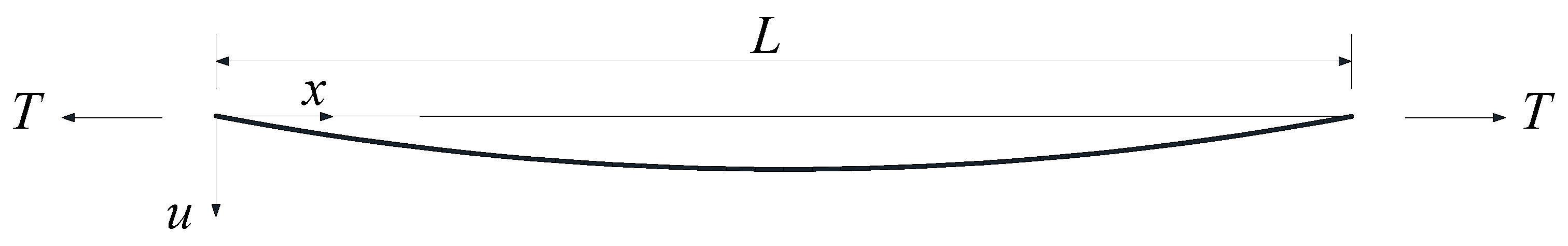
The coordinate system of a tensioned cable is illustrated in Figure 1. When ignoring the influences of the sag and damping, Formula (1) is the free vibration equation of cables.
where u is the displacement of various points of cables at moment t, and m, L, EI, and T represent the linear density, length, flexural stiffness, and the tension, respectively, and are all constants, that is, they do not change with time and location.

Figure 1.
Coordinate system of a tensioned cable.
The equation is solved by separation of variables. The general solution is
where Ai (i =1, 2, 3, 4) is an undetermined coefficient related to the boundary condition, and ω is the angular frequency of vibration of the cable.
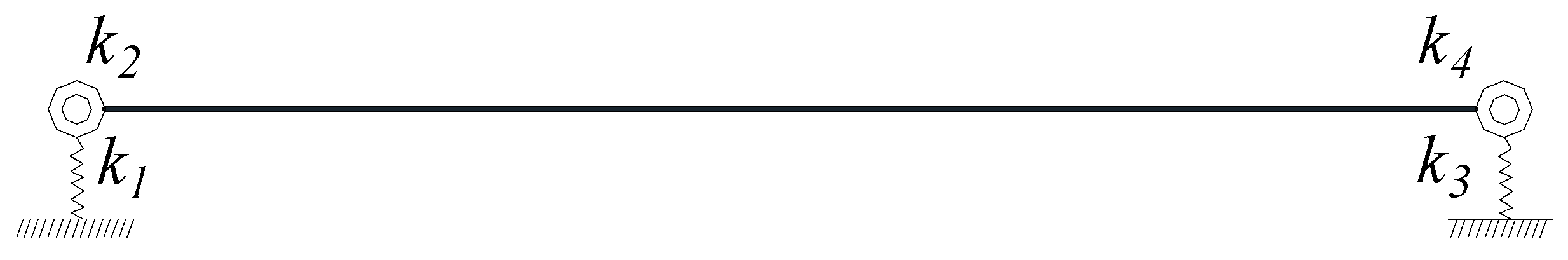
When there are elastic supports at both ends of a cable, the boundary condition is shown in Figure 2, that is,
where k1 and k3 are the vertical support stiffness at either ends of a cable, respectively, and k2 and k4 are the rotational restraint stiffness at either end of a cable, respectively.
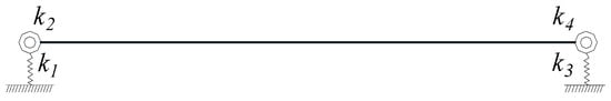
Figure 2.
General boundary conditions.
Under the hinged–hinged boundary condition, by setting k1= k3 = ∞ and k2 = k4 = 0, the following frequency equation is obtained:
Meanwhile, the explicit relationship between the cable tension and frequency under the hinged–hinged boundary condition is determined as follows:
where fn is the nth-order natural vibration frequency.
Under the fixed–hinged boundary condition, the following is obtained when k1 = k3= ∞, k2 = ∞, and k4 = 0:
Under the fixed–fixed boundary condition, k1 = k3 = k2 = k4 = ∞ is set, and the following frequency equation is determined:
When both ends of the cable have arbitrary rotational stiffness, that is, k1 = k3 = ∞, the frequency equation is obtained by substituting Equation (4) into Equation (2):
The physical parameters of the cable are substituted into Equations (6), (8), and (9), thus ascertaining vibration angular frequencies ωnss, ωnfh, and ωnff of the cable with hinged–hinged, fixed–hinged, and fixed–fixed boundary conditions, respectively; n is the order of the mode of vibration. Equations (8)–(10) are transcendental, so no explicit solution can be obtained.
2.2. Fixed–Fixed Boundary Condition
Parameters of some representative booms and cables are listed in Table 1 and Table 2, in which ξ is a dimensionless parameter that reflects the relative flexural stiffness of cables, as expressed by Equation (11) [18]. The lower the value of ξ is, the greater the relative stiffness of cables. Given m, L, EI, and T, the frequency ratio (zn) of cables with a fixed–fixed boundary condition to those with a hinged–hinged boundary condition can be obtained by combining Equations (6) and (9), as expressed by Equation (12).

Table 1.
Parameters pertaining to booms.
Table 2.
Parameters pertaining to cables.
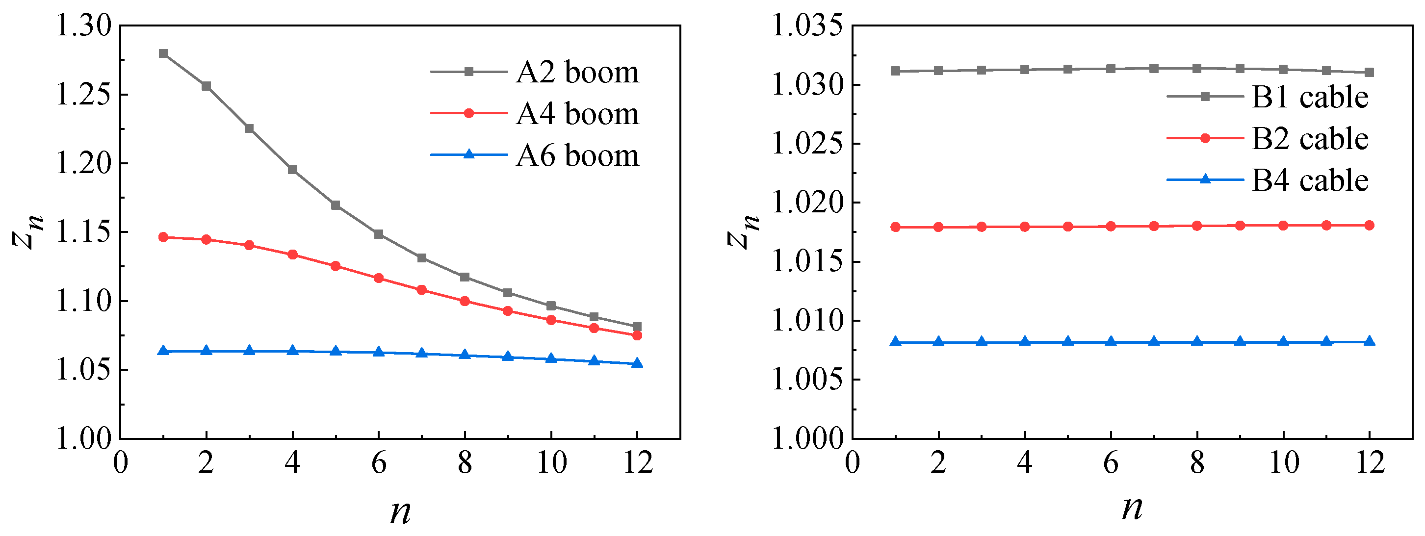
The frequency ratios (zn) of booms A2, A4, and A6 and cables B1, B2, and B3 are analyzed in Figure 3. It can be seen from Figure 3 that the smaller the ξ value of booms is, the greater the frequency ratio (zn), and the frequency ratio declines with rising order. The frequency ratios of various orders of the same cable are basically identical, and the values of zn of cables B1, B2, and B4 reduce successively.
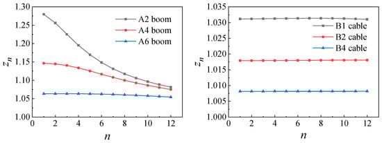
Figure 3.
The frequency ratios of booms and cables.
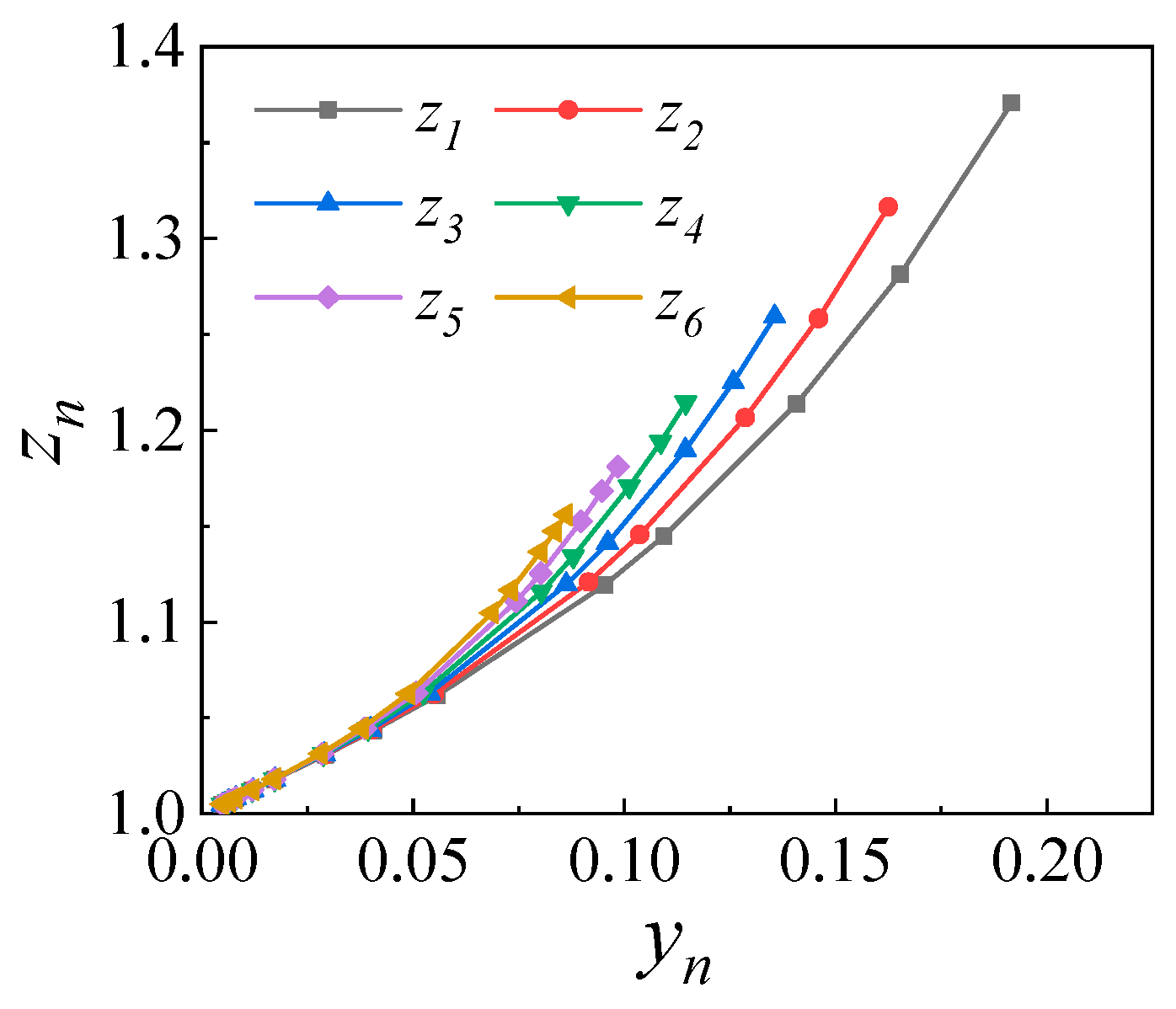
A dimensionless parameter (yn) is proposed, as expressed by Equation (13), and the yn–zn relationship is fitted. On this basis, the frequency ratio (zn) can be calculated with unknown tension. Equation (12) can be used to calculate the frequency ratio (zn) of various orders of cables with different values of ξ; the yn–zn relationship curves of the first six frequencies are shown in Figure 4. Through polynomial fitting, various possible combinations of first-order to fourth-order polynomials are compared. Considering the computation accuracy and for the convenience of application, the combination of the first-order and third-order polynomials is fitted, and the fitting formula for the frequency ratio (zn) of the first six orders is expressed by Equation (14). The solid line in Figure 4 denotes the results arising from use of the regression formula, which conforms to the theoretical calculation results.
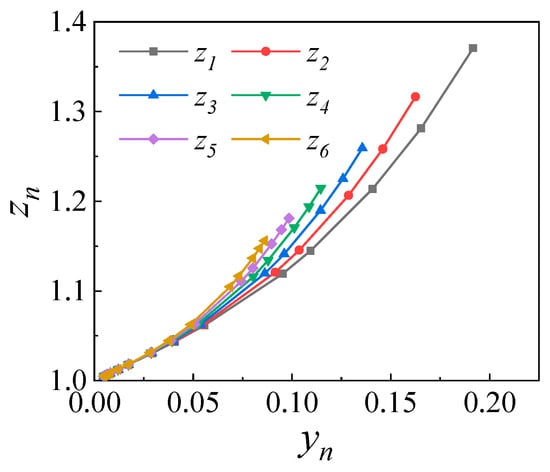
Figure 4.
yn–zn relationship curves.
The unified calculation formula for the frequency ratio (zn) is further fitted, as shown in Equation (15), according to which the calculation formula for tensions is obtained as Equation (16).
2.3. Fixed–Hinged Boundary Condition
The theoretical frequency ratio() of cables with fixed–hinged boundary conditions to those with hinged–hinged boundary conditions can be obtained (Equation (17)) by combining Equations (6) and (8).
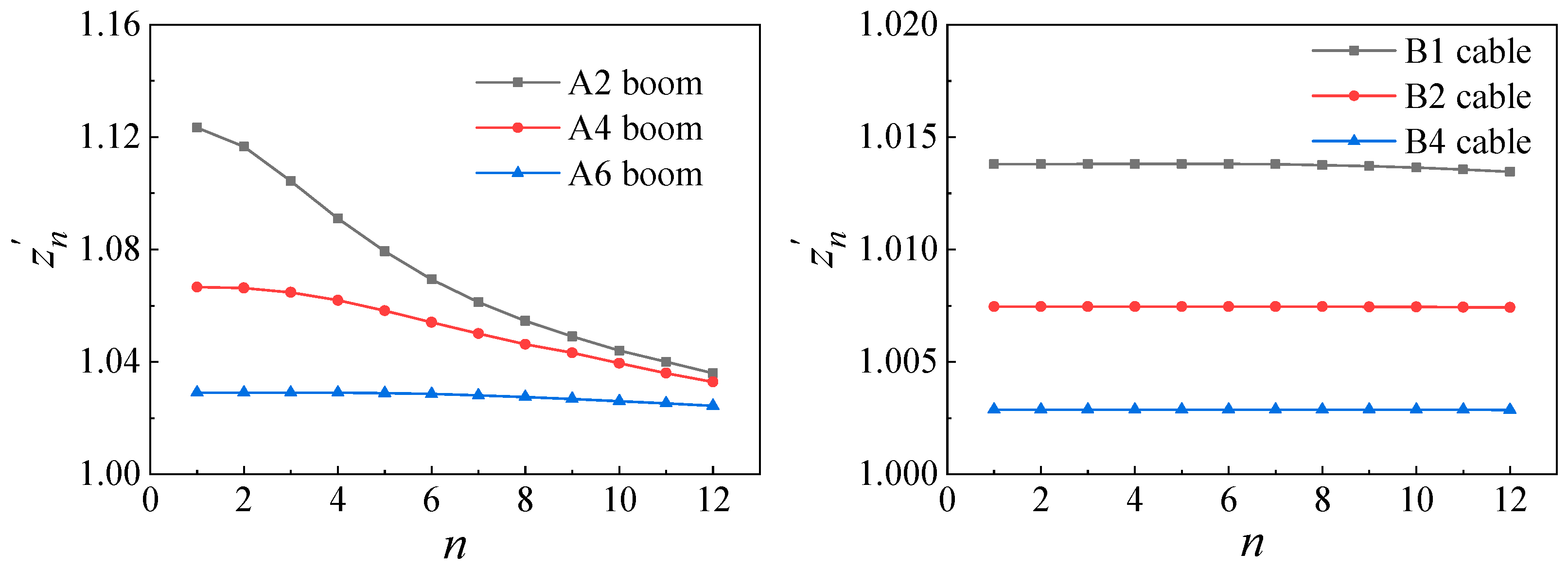
The theoretical frequency ratio() is calculated (Figure 5) according to the physical parameters of cables in Table 1 and Table 2. The theoretical frequency ratios() of booms A2, A4, and A6 increase with decreasing ξ, while they reduce with increasing order of frequency. The theoretical frequency ratios() of cables B1, B2, and B4 decrease successively, while their individual frequency ratios of various orders are similar.

Figure 5.
Frequency ratios of booms and cables.
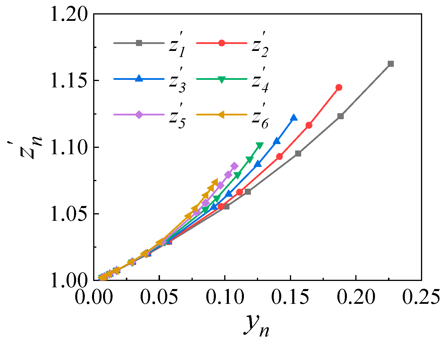
By using the dimensionless parameter (yn), the formulae for yn and of the first six frequencies are obtained via polynomial fitting, as expressed by Equation (18). The yn– relationship curves are shown in Figure 6.
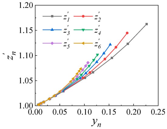
Figure 6.
yn– relationship curve.
The unified calculation (Equation (19)) of the frequency ratio() is obtained by further fitting, thus attaining the calculation formula for the tension of cables with fixed–hinged boundary conditions (Equation (20)).
2.4. Calculation Formula for Tension in a Cable with Arbitrary Rotational End-Restraints
The theoretical frequency of cables with rotational end-restraints and different values of rotational stiffness is calculated using Equation (10). Different boundary conditions of cables are displayed in Figure 7. Boundaries A and C are hinged-rotational and fixed-rotational boundary conditions, respectively, while boundary E indicates arbitrary rotational restraints at both ends, under which the rotational stiffness is k = pEI/L. Therein, EI/L is the linear stiffness, and p is a multiple of rotational stiffness over linear stiffness (EI/L) and is between 0 and 700. The cables in Table 3 were selected to evaluate changes in the fundamental frequency of cables with rotational end-restraints under different values of rotational stiffness. The red point in Figure 8 is the fundamental frequency with p between 0 and 700, and the blue points are the fundamental frequencies with p values of 2, 5, 10, 20, 40, 100, and 500. At p = 500, the error in the fundamental frequency of cables with the fixed–fixed boundary condition is lower than 0.5%, so this can be deemed equivalent to the fixed–fixed boundary condition. The blue points in the figure exhibit uniform frequency variation, so these representative points can be adopted for detailed tension analysis.
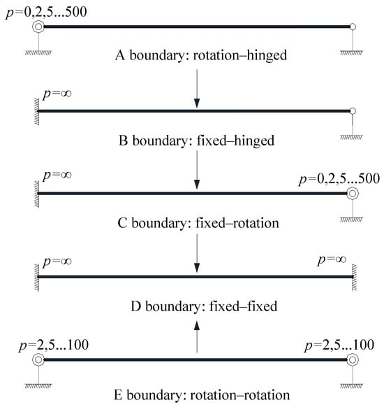
Figure 7.
Cables with different boundary conditions.
Table 3.
Parameters pertaining to the analyzed booms.
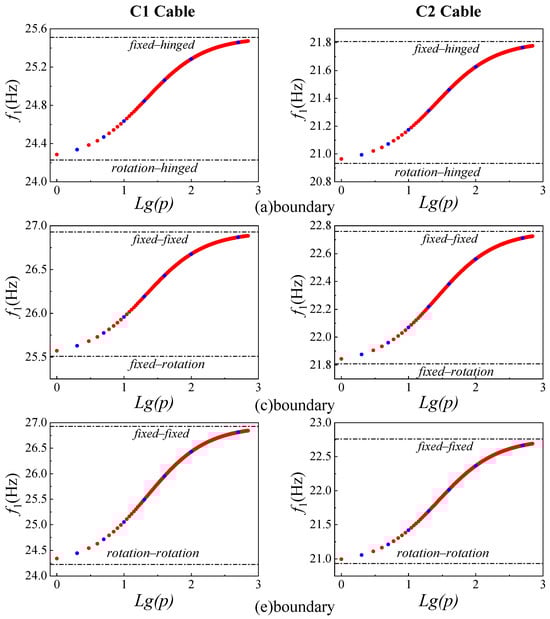
Figure 8.
Fundamental frequencies of cables C1 and C2.
Equation (16) is deduced from the fixed–fixed boundary condition of cables. In fact, apart from fixed–fixed and hinged–hinged boundary conditions, the boundary of cables can also show rotational support somewhat between the two. Summarizing the analysis in Section 2.2 and Section 2.3 shows that, for the frequency ratios of various orders of a cable, the of the cable with a fixed–hinged boundary condition is smaller than the zn of that with the fixed–fixed boundary condition. In addition, as ξ increases, the frequency ratios of various orders of the cable with the two boundary conditions tend to be the same. Therefore, the boundary coefficient(λ) is introduced to assume 1/zn2 = λ in Equation (16). In this way, the tension in cables with boundary conditions involving arbitrary rotational restraint stiffness at both ends can be written as follows:
According to Equation (21), each equation has two unknown quantities, namely T and λ. Two arbitrary frequencies are substituted into Equation (21) to obtain the following linear equation set:
Given the EI, the tension (T) and boundary coefficient(λ) can be obtained by solving the equation set. The cable in Table 3 is analyzed, at both ends of which different rotational restraints are set, and the value of rotational stiffness is valued in the range of 0~500 EI/L. In the table, k2 and k4 are the multiples of rotational restraint stiffness at either end over linear stiffness EI/L, respectively, and they are valued to be 0, 2, 5, 10, 20, 40, 100, and 500, which are combined to obtain 36 boundary conditions. The tension is computed using the above method, and the errors are listed in Table 4, Table 5, Table 6 and Table 7.
Table 4.
Computation errors of cable C1 (Formula (22); i = 1 and j = 2) (%).
Table 5.
Computation errors of cable C1 (Formula (22); i = 2 and j = 3) (%).
Table 6.
Computation errors of cable C2 (Formula (22); i = 1 and j =2) (%).
Table 7.
Computation errors of cable C2 (Formula (22); i = 2 and j = 3) (%).
Table 4, Table 5, Table 6 and Table 7 show that at i = 1 and j = 2, the computation error of tension using Equation (22) is lower than that at i = 2 and j = 3, and the error for cable C1 is slightly larger. In the case of i = 1 and j = 2, the tension errors under six boundary conditions exceed 5%; under i = 2 and j = 3, the tension errors under 14 boundary conditions exceed 5%, with a maximum error of 6.84%. In comparison, the maximum tension error for cable C2 is only 4.79%, which is less than 5%.
The first five frequencies of cables are studied. The tension in a cable is calculated by substituting the ith and jth (condition kij) natural vibration frequencies under 36 boundary conditions into Equation (22), thus obtaining 36 relative errors in the tensions. The largest error is defined as eij (the black triangular point in Figure 9). Errors under each condition are shown in Figure 9. A total of 10conditions are set for each cable, so there are a total of 360 relative errors.
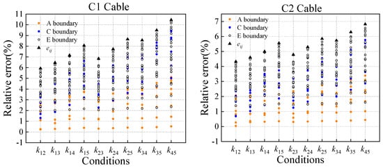
Figure 9.
Tension errors in cables C1 and C2 under each condition.
Among the 360 errors of cable C1, 167 errors exceed 5%, which account for 46.4%; the optimal computation accuracy is obtained under k12 among the ten conditions, under which some errors are also larger than 5% though. Only 39 errors of cable C2 exceed 5%, which account for 10.83%. The relative errors of tensions under conditions k12, k13, k14, and k23 are all below 5%. Additionally, the eij values of the two cables under ten conditions were compared, and the results show that the eij values of cable C1 are all larger than those of cable C2. This indicates that as ξ increases, Equation (22) is found to be more accurate.
The relative tension errors of cables C1 and C2 under boundaries A, C, and E are displayed in Figure 9. The majority of errors of the two cables under boundary A are smaller than 5%. To be specific, the errors of cable C2 under boundary A are all lower than 4%, suggesting favorable computation accuracy. Among the 70 errors of cable C1 under boundary C, 36 errors are higher than 5%, which exceeds 50%. Except for four errors of cable C2 under conditions k35 and k45 that are larger than 5%, errors under other conditions are all lower than 5%, showing moderate computational accuracy. The accuracy of the two cables under boundary E is lower, and the eij values under the ten conditions are all obtained under boundary E. The relative tension errors of cable C2 under four conditions (k12, k13, k14, and k23) are all under 5%.
The cables in Table 8 are analyzed, and emax1 is defined as the maximum eij (a total of 10 conditions). Meanwhile, the fundamental frequencies of cables are substituted into Equation (7) to calculate the tensions of cables under 36 boundary conditions. The maximum relative tension error is defined as emax2. The results are summarized in Table 9.
Table 8.
Parameters pertaining to the analyzed cables.
Table 9.
Cable tension errors (%).
It can be seen from Table 9 that when Equation (22) is used to calculate the tension using an arbitrary set of two of the first five natural vibration frequencies, the emax1 of cable C2 is 6.82%, and e12, e13, e14, and e23 are all no larger than 5%; with regard to cables with 25 ≤ ξ ≤ 114, as ξ increases, emax1 decreases and tends toward 1%; if 114 ≤ ξ ≤ 200, emax1 increases with increasing ξ, whereas, emax2 continues to decrease with increasing ξ, and the emax2 values of cables B3 and B4 are both less than 2%, suggesting slight influences of changes in the boundary conditions on cables with large ξ values. A comparison of the emax1 and emax2 values of the cables in Table 9 shows that when the ξ value of cables is approximately 165, emax1 and emax2 are both less than 2%; as ξ continues to increase, emax1 increases, while emax2 decreases.
According to the above analysis, the relative tension errors of cables with arbitrary rotational stiffness at both ends calculated by Equation (22) under conditions k12, k13, k14, and k23 are all below 5% when 25 ≤ ξ ≤ 165; if 34 ≤ ξ ≤ 165, the relative errors are all below 4% when calculating the tension using the first five natural vibration frequencies predicted using Equation (22); as ξ increases, the accuracy of the formula is improved.
3. Results and Discussion
3.1. Verification of Calculation under the Fixed–Fixed Boundary Condition
To verify the accuracy and range of application of the proposed calculation formulae for tensions, the booms and cables in Table 1 and Table 2 were selected to calculate their tensions using the fundamental frequency, and some booms and cables were selected to calculate their tensions using the higher-order frequencies. The results were compared using the following equations.
Huang provides the following formulae for the fixed–fixed boundary condition and the fixed–hinged boundary condition:
The following formula is for the fixed–fixed boundary condition:
The following formula is for the fixed–hinged boundary condition:
Fang’s formula is expressed as follows:
Ren’s formula is expressed as follows:
Zui’s formula is expressed as follows:
The tension errors in booms and cables calculated based on the fundamental frequency are shown in Figure 10; the errors in booms calculated using Ren’s formula are below 2.5%, indicating high accuracy; the use of Zui’s formula yields similar results to Ren’s formula in terms of computational accuracy; the tension errors are all below 2.5% when Fang’s formula, Huang’s formula, and Equation (16) are used for computation, among which Equation (16) performs best on the whole and shows tension errors of less than 1% for booms. When using the five formulae to calculate tensions of cables with large ξ values, the tensions calculated by five formulae show subtle differences, with errors all less than 2.5%.
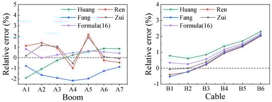
Figure 10.
Tension errors when using the five formulae.
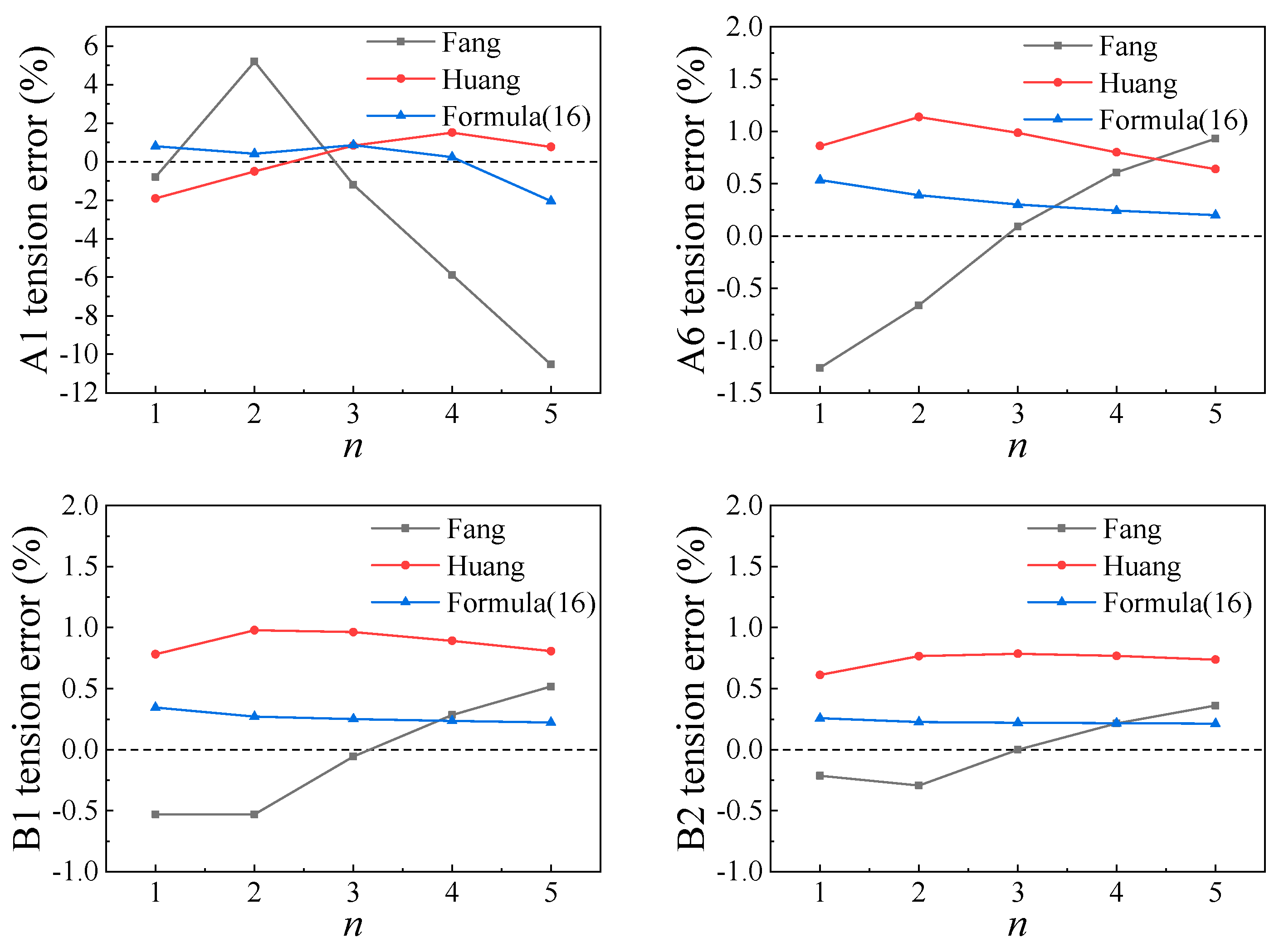
To verify the accuracy of Equation (16) in calculating tensions using the higher-order frequencies, the first five frequencies of booms were substituted into Fang’s formula, Huang’s formula, and Equation (16) to compute tensions. The relative errors are illustrated in Figure 11. The tensions of boom A1 calculated by Fang’s formula are highly discrete, which is indicative of large tension errors in the computation using higher-order frequencies, with the maximum tension error exceeding 10%. The tension errors of booms calculated by Huang’s formula and Equation (16) based on various frequencies are all lower than 2.5%, and Equation (16) performs better on the whole. Therefore, Equation (16) has the best computational accuracy and a wider range of applications.
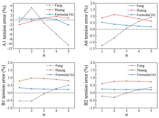
Figure 11.
Tension errors of fixed–fixed boundary booms and cables.
3.2. Verification of Calculation under the Fixed–Hinged Boundary Condition
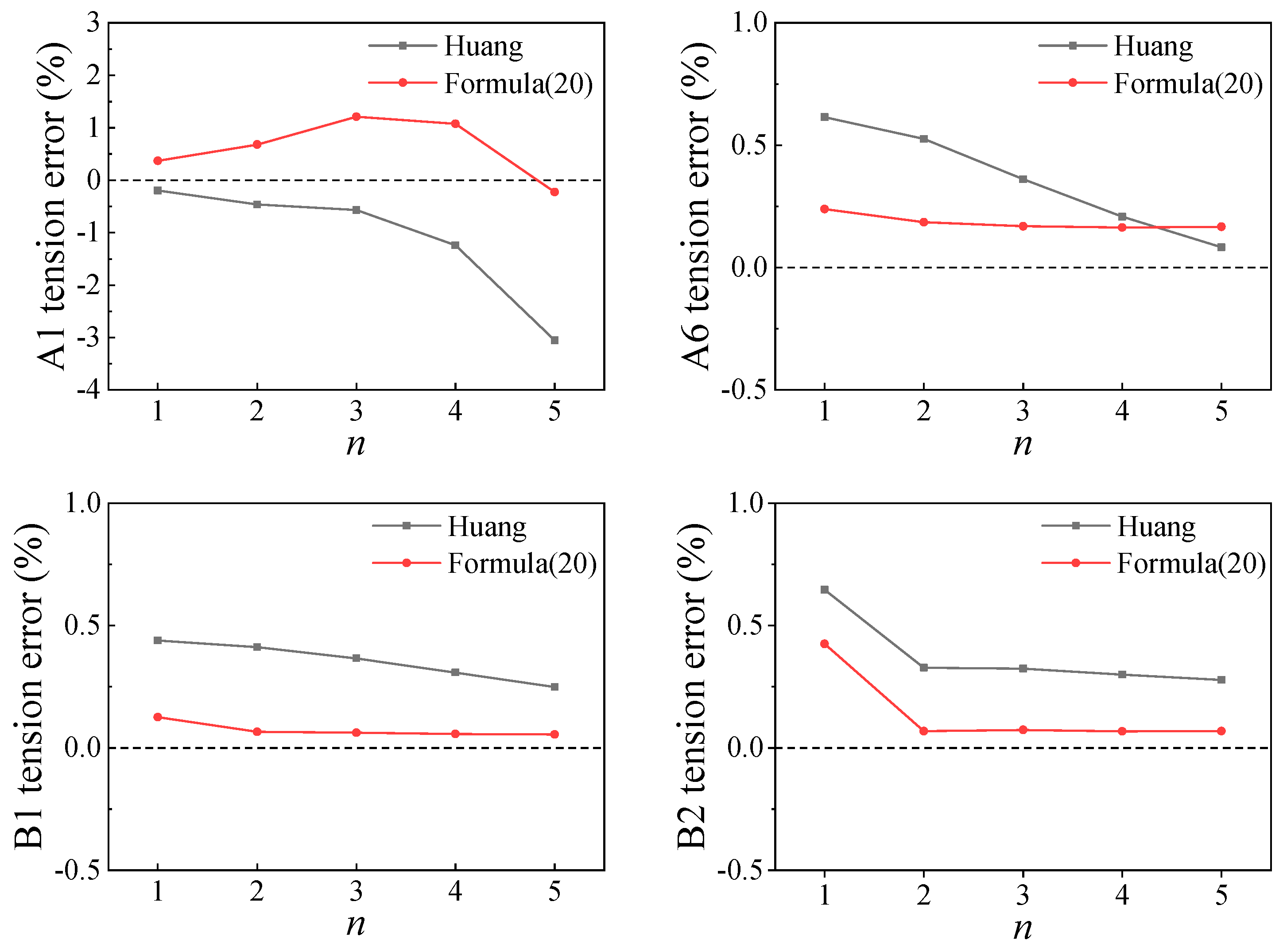
Booms A1 and A6 and cables B1 and B2 were analyzed. The errors of tensions calculated by different formulae with the real tensions are shown in Figure 12. The relative tension errors of boom A1 computed by Huang’s formula increase with rising order, and the maximum relative error is −3.05%, while the relative tension errors calculated by Equation (20) are less than 1.5%; the tension errors of boom A2 and cables B1 and B2 are always less than 1% when calculated using the two formulae, indicating the stable computational accuracy of the two. In comparison, Equation (20) is found to have higher computational accuracy under the fixed–hinged boundary condition.
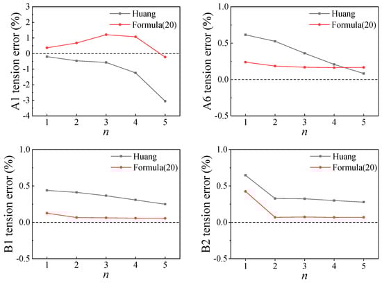
Figure 12.
Tension errors of fixed–hinged boundary booms and cables.
3.3. Verification of Calculation under Arbitrary Rotational Restraint at Each End
The finite element model and data reported in previous research [16] were used to verify Equation (22). The physical parameters of booms are listed in Table 10; the boundary conditions and multi-order frequencies are listed in Table 11.
Table 10.
Parameters pertaining to the analyzed boom.
Table 11.
Frequencies (Hz).
Given the multi-order frequencies and physical parameters of the boom, Equation (22) can be used to identify the cable tension. Table 12 and Table 13 separately show the tension errors of Formula (22) with real tensions under fixed–fixed and fixed–hinged boundary conditions, which are also compared with the calculation results of Equations (16) and (20). It can be seen from the table that the errors are always less than 0.2% when computed by Equations (16) and (20) based on the first five frequencies; the maximum relative error of tensions calculated by Equation (22) according to the first and second frequencies is 1.7%, and the relative error is always within 1% when computing tensions using frequencies other than the fundamental frequency.
Table 12.
Relative errors of T1 and T2 (fixed–fixed).
Table 13.
Relative errors of T1 and T2 (hinged–fixed).
The analysis objects in [16] were booms with the inclination of 90°, which do not sag. Here, the boom in Table 10 was taken as the object to analyze the accuracy of Equation (22) for the tensions of cables under fixed–fixed boundary conditions and different inclinations so as to study the influence of the sag thereon. Table 14 lists the relative errors of tensions of cables with seven inclinations calculated by Equation (22). Under condition k12, that is, calculating the tension using Equation (22) according to the first and second frequencies, the relative error exceeds 30% when the inclination is 0; the error is large under the condition of calculating the tension using Formula (22) based on the first frequency when the inclination is small, while if the inclinations are 75° and 90°, the errors are always less than 1%.
Table 14.
Tension errors for cables with different inclinations (%).
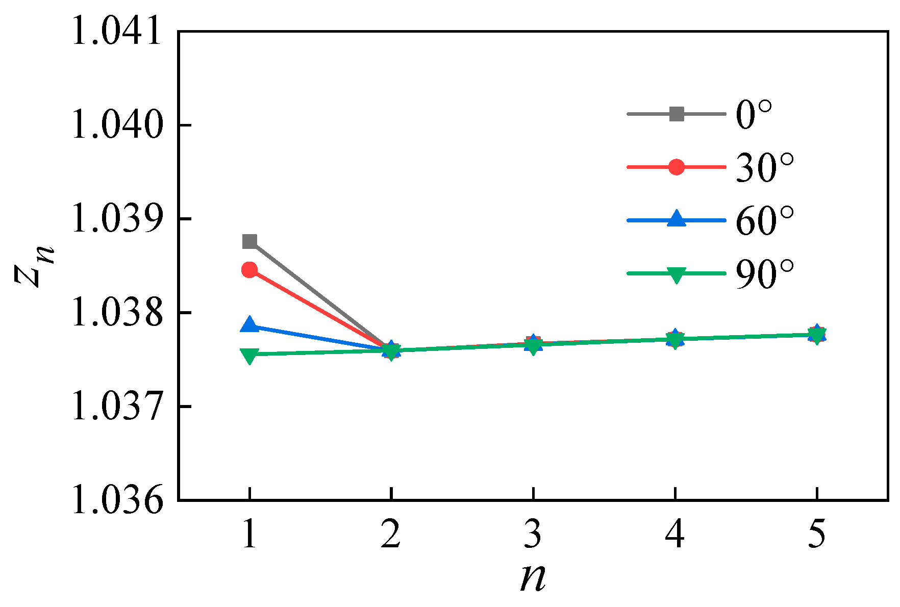
The reason for the poor computation accuracy of Equation (22) based on the first frequency under small inclinations was ascertained. The frequency ratios of cables with fixed–fixed boundary conditions to those with hinged–hinged boundary conditions under inclinations of 0°, 30°, 60°, and 90° were calculated (Figure 13); at an inclination of 90°, the frequency ratios of the first five orders of cables are consistent, while as the inclination decreases, the frequency ratio of the first order enlarges abruptly, while those of other orders remain largely unchanged. Therefore, when calculating tensions using Equation (22) based on the first frequency, the smaller the inclination, the greater the changes in the frequency ratio of the first order, which incurs larger tension errors. Considering this, when calculating the tension in an inclined cable using Equation (22) in engineering applications, using frequencies other than the fundamental frequency can improve the computational accuracy.
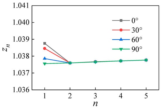
Figure 13.
The frequency ratios of cables.
3.4. Engineering Applications
3.4.1. Hedong Cable-Stayed Bridge
To validate the effectiveness of Equation (16), measured vibration data from [16] were adopted for analysis. The data were acquired from Hedong bridge in Guangzhou Province, China.
Hedong bridge is a double-tower, three-span (144 + 360 + 144 m), cable-stayed bridge that possesses 72 pairs of stay cables. The spacing between two adjacent cables is 9.5 m. The shortest and longest cables (C18 and C36, respectively) were analyzed, and their physical parameters are listed in Table 15. The inertia moments of cables were calculated by using the material mechanics method, and the cable frequencies were determined according to the frequency spectra of measured acceleration–time curves.
Table 15.
Parameters pertaining to the cables on Hedong bridge [16].
Table 16 compares the cable tensions calculated by different practical formulae, the results of which are similar to the designed cable tensions, with relative errors below 2%. Apparently, Fang’s formula and Equation (16) are both applicable to the computation of cable tensions, while computation using Equation (16) is simpler.
Table 16.
Comparison of computed cable tensions on Hedong bridge (unit: m).
3.4.2. Anchor-Span Strands on Hangrui Dongting Bridge
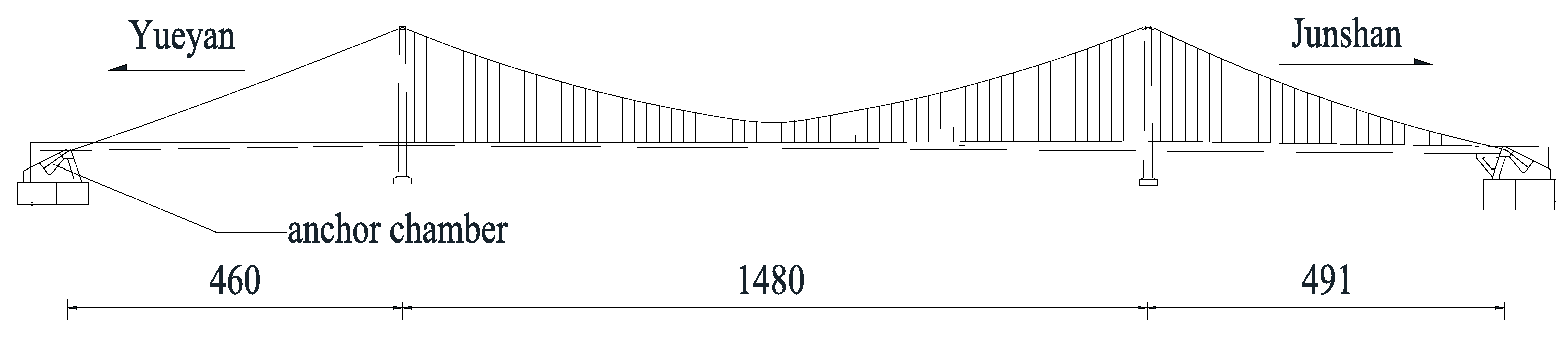
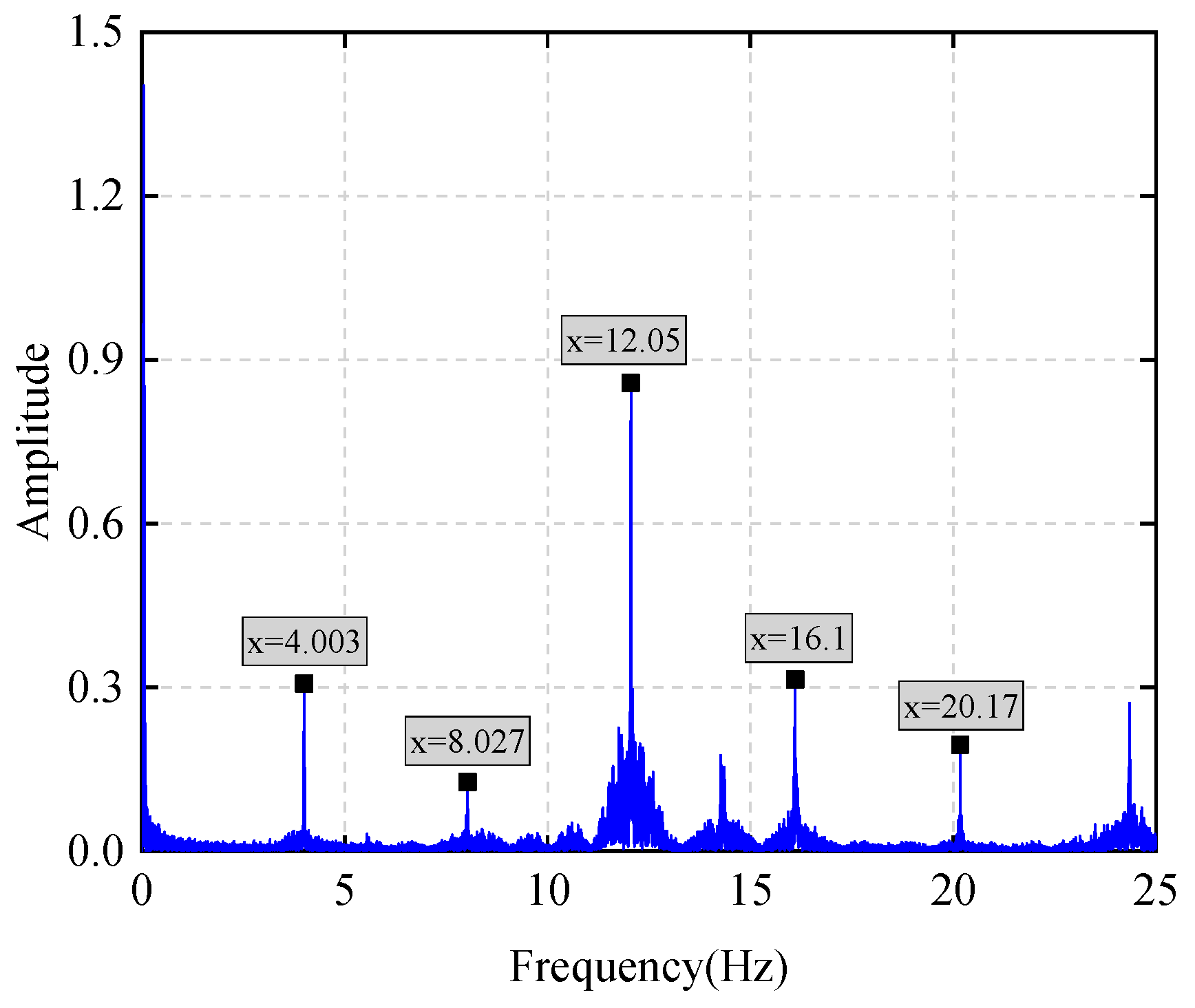
Hangrui Dongting bridge, located at the confluence of Dongting Lake and the Yangtze River, is an important project of the Linwu–Yueyang expressway. The bridge layout is displayed in Figure 14. The anchor span on the Yueyang City side and the strand arrangement are shown in Figure 15. Strand #85 was studied and the relevant parameters of which are shown in Table 17. The acceleration data of the strand sampled at a frequency of 100 Hz within 10 min were analyzed by fast Fourier transform (FFT), obtaining the frequency spectrum (Figure 16).
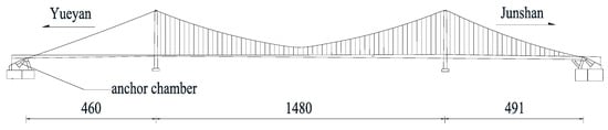
Figure 14.
Side view of Hangrui Dongting bridge (unit:m).
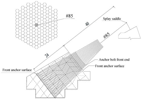
Figure 15.
Anchor span arrangement (unit: m).
Table 17.
Parameters pertaining to the analyzed cable on Hangrui Dongting bridge.
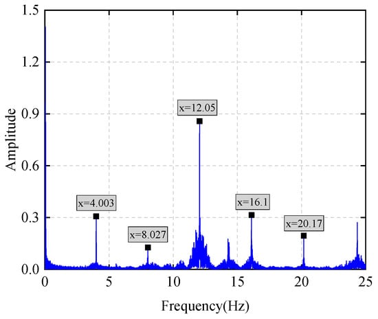
Figure 16.
Amplitude spectrum of acceleration.
Table 18 compares the calculation results of strand tensions of the proposed method and Equation (7). The relative tension errors of strand #85 calculated by Equation (7) at various frequencies are consistent and reach 2.17%; when calculating the strand tension based on f1 and f2 using the proposed method, the relative error is 36%, which is caused by the significant influence of the first frequency on sag according to the aforementioned analysis. When calculating the strand tension using the higher-order frequency, the results have a relative error lower than 0.6% with the design value. The computational accuracy of the two practical formulae is lower than 5%, and Equation (22) returns a higher accuracy.
Table 18.
Comparison of computed cable tensions on Hangrui Dongting bridge.
4. Conclusions
The frequency characteristic equations of cables with fixed–fixed, fixed–hinged, and hinged–hinged boundary conditions were first constructed. The frequency ratios of cables with fixed–fixed and fixed–hinged boundary conditions to those with hinged–hinged boundary conditions were obtained. In addition, a dimensionless parameter (yn) was introduced. By fitting the explicit relationship between the frequency ratio and the dimensionless parameter (yn), the calculation formulae for the tensions of cables with fixed–fixed and fixed–hinged boundary conditions were deduced. Changes in the frequency ratios of various orders of cables with different ξ values were analyzed in detail. The boundary coefficient(λ) was introduced, and a novel method for calculating the tensions of cables with arbitrary rotational restraints at both ends was proposed, which was proven to be effective with reference to practical engineering examples.
- (1)
- The dimensionless parameter (yn) was proposed, and its relationship with the frequency ratio was fitted. Accordingly, the calculated frequency ratios of the first six orders of cables with different ξ values were attained, which are similar to the theoretical values. This relationship can be used to calculate the frequency ratios of cables with fixed–fixed and fixed–hinged boundary conditions to those with hinged–hinged boundary conditions when the tension is unknown.
- (2)
- Practical formulae for calculating the tensions of cables with fixed–fixed and fixed–hinged boundary conditions were proposed based on the frequency ratio, which can be used to compute cable tensions with ξ values not lower than 6.9 based on multi-order frequencies. The tensions of obviously sagged cables calculated based on the fundamental frequency have a relative error smaller than 2.5%, while the error can be kept below 1.5% when higher-order frequencies are used for computation. The two formulae both result in high computational accuracy and a wide range of applications. In engineering examples, the tension errors of two stay cables are both lower than 2%, and the results are more accurate than the tensions calculated by Fang’s formula. This indicates that the proposed formulae are applicable to cables with different values of bending stiffness and sag.
- (3)
- Changes in the frequency ratios of cables with fixed–fixed and fixed–hinged boundary conditions to those with hinged–hinged boundary condition were evaluated. The results indicate that as ξ increases, the frequency ratios of various orders of cables tend to be the same. The boundary coefficient(λ) was introduced. Given the stiffness and two arbitrary natural vibration frequencies of cables, the tension and boundary coefficient(λ) can be obtained through linear regression. This method can be used to calculate the tension of cables with 25 ≤ ξ ≤ 165 and with unknown rotational restraints at both ends. When computing the tension using any two of the first five frequencies, most tension errors are below 5%; if the sag effect of cables is considered, calculations based on frequencies other than the fundamental frequency ensure that most errors are below 5%. The computational accuracy is highest when calculating the tension using the second and third frequencies, with the errors both less than 5%.
Author Contributions
Methodology, B.G. and S.T.; software, B.G. and M.Z.; validation, B.G. and X.Z.; investigation, B.G. and M.Z.; data curation, B.G. and G.Z.; writing—original draft preparation, B.G. and M.Z.; writing—review and editing, S.T. and X.Z.; funding acquisition, S.T. All authors have read and agreed to the published version of the manuscript.
Funding
This research was funded by the Scientific Research Fund of Hunan Provincial Education Department(20K126), the National Natural Science Foundation of China (51508488), the Hunan Provincial Natural Science Foundation of China (2019JJ50605), and the High-level Talent Gathering Project in Hunan Province (2019RS1059).
Data Availability Statement
The testing and analysis data used to support the findings reported in this study are included within the article.
Conflicts of Interest
Author Guogang Zhang was employed by the company Hunan Provincial Communications Planning, Survey & Design Institute Co., Ltd. The remaining authors declare that the research was conducted in the absence of any commercial or financial relationships that could be construed as a potential conflict of interest.
References
- Haji Agha Mohammad Zarbaf, S.E.; Norouzi, M.; Allemang, R.J.; Hunt, V.J.; Helmicki, A.; Nims, D.K. Stay Force Estimation in Cable-Stayed Bridges Using Stochastic Subspace Identification Methods. J. Bridge Eng. 2017, 22, 04017055. [Google Scholar] [CrossRef]
- Rebelo, C.; Júlio, E.; Varum, H.; Costa, A. Cable Tensioning Control and Modal Identification of a Circular Cable-Stayed Footbridge. Exp. Tech. 2009, 34, 62–68. [Google Scholar] [CrossRef]
- Wang, J.; Liu, W.; Wang, L.; Han, X. Estimation of main cable tension force of suspension bridges based on ambient vibration frequency measurements. Struct. Eng. Mech. 2015, 56, 939–957. [Google Scholar] [CrossRef]
- Nazarian, E.; Ansari, F.; Zhang, X.; Taylor, T. Detection of Tension Loss in Cables of Cable-Stayed Bridges by Distributed Monitoring of Bridge Deck Strains. J. Struct. Eng. 2016, 142, 04016018. [Google Scholar] [CrossRef]
- Yim, J.; Wang, M.L.; Shin, S.W.; Yun, C.-B.; Jung, H.-J.; Kim, J.-T.; Eem, S.-H. Field application of elasto-magnetic stress sensors for monitoring of cable tension force in cable-stayed bridges. Smart Struct. Syst. 2013, 12, 465–482. [Google Scholar] [CrossRef]
- Syamsi, M.I.; Wang, C.-Y.; Nguyen, V.-S. Tension force identification for cable of various end-restraints using equivalent effective vibration lengths of mode pairs. Measurement 2022, 197, 111319. [Google Scholar] [CrossRef]
- Fu, Z.; Ji, B.; Wang, Q.; Wang, Y. Cable Force Calculation Using Vibration Frequency Methods Based on Cable Geometric Parameters. J. Perform. Constr. Facil. 2017, 31, 04017021. [Google Scholar] [CrossRef]
- Xu, Y.; Xie, Y.; Chen, S.; Zhu, M. Evaluation of the Cable Force by Frequency Method for the Hybrid Boundary between the Ear Plate and the Anchor Plate. Buildings 2022, 12, 1853. [Google Scholar] [CrossRef]
- Kim, B.H.; Park, T. Estimation of cable tension force using the frequency-based system identification method. J. Sound Vib. 2007, 304, 660–676. [Google Scholar] [CrossRef]
- Wang, R.; Gan, Q.; Huang, Y.; Ma, H. Estimation of Tension in Cables with Intermediate Elastic Supports Using Finite-Element Method. J. Bridge Eng. 2011, 16, 675–678. [Google Scholar] [CrossRef]
- Liao, W.Y.; Ni, Y.Q.; Zheng, G. Tension Force and Structural Parameter Identification of Bridge Cables. Adv. Struct. Eng. 2016, 15, 983–995. [Google Scholar] [CrossRef]
- Ceballos, M.A.; Prato, C.A. Determination of the axial force on stay cables accounting for their bending stiffness and rotational end restraints by free vibration tests. J. Sound Vib. 2008, 317, 127–141. [Google Scholar] [CrossRef]
- Ni, Y.Q.; Ko, J.M.; Zheng, G. Dynamic Analysis of Large-Diameter Sagged Cables Taking into Account Flexural Rigidity. J. Sound Vib. 2002, 257, 301–319. [Google Scholar] [CrossRef]
- Zui, H.; Shinke, T.; Namita, Y. Practical Formulas for Estimation of Cable Tension by Vibration Method. J. Struct. Eng. 1996, 122, 651–656. [Google Scholar] [CrossRef]
- Fang, Z.; Wang, J.-q. Practical Formula for Cable Tension Estimation by Vibration Method. J. Bridge Eng. 2012, 17, 161–164. [Google Scholar] [CrossRef]
- Huang, Y.-H.; Fu, J.-Y.; Wang, R.-H.; Gan, Q.; Liu, A.-R. Unified Practical Formulas for Vibration-Based Method of Cable Tension Estimation. Adv. Struct. Eng. 2016, 18, 405–422. [Google Scholar] [CrossRef]
- Huang, Y.H.; Fu, J.Y.; Wang, R.H.; Gan, Q.; Rao, R.; Liu, A.R. Practical formula to calculate tension of vertical cable with hinged-fixed conditions based on vibration method. J. Vibroeng. 2014, 16, 997–1009. [Google Scholar]
- Ren, W.-X.; Chen, G.; Hu, W.-H. Empirical formulas to estimate cable tension by cable fundamental frequency. Struct. Eng. Mech. 2005, 20, 363–380. [Google Scholar] [CrossRef]
- Yan, B.; Yu, J.; Soliman, M. Estimation of Cable Tension Force Independent of Complex Boundary Conditions. J. Eng. Mech. 2015, 141, 06014015. [Google Scholar] [CrossRef]
- Chen, C.-C.; Wu, W.-H.; Chen, S.-Y.; Lai, G. A novel tension estimation approach for elastic cables by elimination of complex boundary condition effects employing mode shape functions. Eng. Struct. 2018, 166, 152–166. [Google Scholar] [CrossRef]
- Chen, C.C.; Wu, W.H.; Leu, M.R.; Lai, G.L. Tension determination of stay cable or external tendon with complicated constraints using multiple vibration measurements. Measurement 2016, 86, 182–195. [Google Scholar] [CrossRef]
- Chen, C.C.; Wu, W.H.; Huang, C.H.; Lai, G.L. Determination of stay cable force based on effective vibration length accurately estimated from multiple measurements. Smart Struct. Syst. 2013, 11, 411–433. [Google Scholar] [CrossRef]
- Xu, Y.; Zhang, J.; Zhang, Y.; Li, C. A Novel Approach for Cable Tension Monitoring Based on Mode Shape Identification. Sensors 2022, 22, 9975. [Google Scholar] [CrossRef] [PubMed]
- Le, L.X.; Siringoringo, D.M.; Katsuchi, H.; Fujino, Y. Stay cable tension estimation of cable-stayed bridge under limited information on cable properties using artificial neural networks. Struct. Control Health Monit. 2022, 29, e3015. [Google Scholar] [CrossRef]
- Dan, D.-h.; Xia, Y.; Xu, B.; Han, F.; Yan, X.-f. Multistep and Multiparameter Identification Method for Bridge Cable Systems. J. Bridge Eng. 2018, 23, 04017111. [Google Scholar] [CrossRef]
- Zhang, W.M.; Wang, Z.W.; Feng, D.D.; Liu, Z. Frequency-based tension assessment of an inclined cable with complex boundary conditions using the PSO algorithm. Struct. Eng. Mech. 2021, 79, 619–639. [Google Scholar] [CrossRef]
- Gai, T.T.; Yu, D.H.; Zeng, S.; Lin, J.C.W. An optimization neural network model for bridge cable force identification. Eng. Struct. 2023, 286, 116056. [Google Scholar] [CrossRef]
- Ma, L. A highly precise frequency-based method for estimating the tension of an inclined cable with unknown boundary conditions. J. Sound Vib. 2017, 409, 65–80. [Google Scholar] [CrossRef]

Disclaimer/Publisher’s Note: The statements, opinions and data contained in all publications are solely those of the individual author(s) and contributor(s) and not of MDPI and/or the editor(s). MDPI and/or the editor(s) disclaim responsibility for any injury to people or property resulting from any ideas, methods, instructions or products referred to in the content. |
© 2024 by the authors. Licensee MDPI, Basel, Switzerland. This article is an open access article distributed under the terms and conditions of the Creative Commons Attribution (CC BY) license (https://creativecommons.org/licenses/by/4.0/).