Study on the Equivalent Stiffness of a Local Resonance Metamaterial Concrete Unit Cell

Abstract

This paper addresses the pressing scientific problem of accurately predicting the equivalent stiffness of local resonance metamaterial concrete unit cells. Existing theoretical models often fail to capture the nuanced dynamics of these complex systems, resulting in suboptimal predictions and hindering advancements in engineering applications. To address this deficit, this paper proposes a novel two-dimensional theoretical vibration model that incorporates shear stiffness, a crucial yet often overlooked parameter in previous formulations. Motivated by the need for improved predictive accuracy, this paper rigorously validates a new theoretical model through numerical simulations, considering variations in material parameters and geometric dimensions. The analysis reveals several key findings: firstly, the equivalent stiffness increases with elastic modulus while the error rate decreases, holding geometric parameters and Poisson’s ratio constant. Secondly, under fixed geometric parameters and coating elastic modulus, the equivalent stiffness rises with an increasing Poisson’s ratio, accompanied by a decrease in error rate. Importantly, this paper demonstrates that the proposed model exhibits the lowest error rate across all parameter conditions, facilitating superior prediction of equivalent stiffness. This advancement holds significant implications for the design and optimization of metamaterial structures in various engineering applications for vibration isolation, with promising enhancements of performance and efficiency.

1. Introduction

“Metamaterial” is a general term for composite materials that have artificially designed microstructures and exhibit extraordinary physical properties not found in the natural materials. These composites exhibit unusual properties when interacting with electromagnetic waves [1,2], acoustic waves [3,4,5,6,7,8,9] and elastic waves.

Metamaterial concrete replaces general aggregates in concrete with spherical aggregates formed by composite materials [10,11,12,13]. The spherical aggregates are designed as a layered structure consisting of high-density heavy metal cores and an outer soft coating. The energy dissipation, shock absorption and anti-explosion of the structure are of great significance, and they are mainly used in major engineering fields such as vibration equipment foundations, high-speed railway flat tracks, nuclear power plants and offshore platforms [14,15,16,17,18].

The bandgap is one of the most remarkable features of metamaterial concrete, which can isolate the propagation of specific frequency waves [19,20,21,22,23,24,25]. Many scholars have carried out numerical simulations and experimental studies on the bandgap characteristics and obtained the parameters and laws affecting the bandgap [26,27,28,29,30]. Although these studies have calculated the bandgap values of the concrete cells of metamaterials under different parameter conditions and obtained the corresponding parameter laws, we cannot establish the specific correspondence between the bandgap frequency and the parameter values, and in actual engineering, when facing a project-specific frequency, we cannot directly determine the parameter conditions of the concrete cells of metamaterials, which creates a need to study the specific numerical relationships between equations. Gongye Zhang et al. [31] proposed a new one-dimensional metamaterial model, where they studied a rod-like metamaterial model under an axial end force, with the results showing that compressional deformation occurred at the free end, with counterclockwise torsion. Youchuan Zhou et al. [32] designed a novel three-dimensional mechanical metamaterial with low-frequency bandgaps and a negative Poisson’s ratio, and the bandgap characteristics of the proposed metamaterial were determined computationally, with the mechanism for bandgap occurrence characterized as the local resonance of ligaments and resonators. En Zhang et al. [33] designed the phononic crystal structure of a local resonance composite unit to have good low-frequency characteristics, and they discussed the formation mechanism and influencing factors of the bandgap. Jie Han et al. [34,35,36] established a three-dimensional vibration model based on a one-dimensional spring–mass system model. Bo Zhang et al. [37] proposed a new approach for calculating the effective mass density of a composite containing local resonance units with hard spherical cores, with the calculation based on vibration theory. Nhi Vo et al. [38,39] proposed a dual-meta panel functioning as a sacrificial cladding and conducted a theoretical derivation of the bandgap formulation, which was in good agreement with the numerical model. Junmin Yu et al. [40] produced a bandgap equation derived from the general mass–spring system, where the final bandgap was derived by substituting the system into a serpentine resonator.

According to the existing theoretical formula for determining the bandgap bandwidth, the start and end frequencies of the bandgap are only related to the equivalent stiffness $k$ value and effective masses $M_1$ and $M_2$, and the equivalent stiffness $k$ is one of the most important quantities affecting the value of the bandgap. Accordingly, since the existing research fails to accurately describe the unit cell’s equivalent stiffness, there is a need to carry out an in-depth study of the equivalent stiffness value, determine its calculation formula and verify its accuracy. With those aims, based on the previous research, this paper proposes an improved two-dimensional theoretical vibration model, which is developed by citing two existing theoretical models. By analyzing the geometric dimensions, elastic moduli and Poisson’s ratios of the new model and those from which it is developed, the accuracy of their calculation results is compared using the finite element simulation method.

2. Theoretical Model

2.1. One-Dimensional Vibration Theory Model

The mechanism of bandgap generation in metamaterial concrete monoliths is local resonance. Local resonance is an important phenomenon in phononic crystals, which involves the scattering of phonons due to periodic modulation of the lattice. Within the local resonance region, phonons are damped, creating a local resonance mode and leading to the formation of a phonon bandgap, which prevents phonons from propagating in a specific frequency range.

The equivalent mass is used to describe the mechanical properties of metamaterial concrete. In metamaterial concrete, the basic unit is taken as the research object, as shown in Figure 1. The metamaterial concrete unit cell is simplified to a mechanical model, as shown in Figure 2, where the mass of the mortar matrix is $m_1$, the mass of the core column is $m_2$, the soft coating is equivalent to a spring with a stiffness of $k_{e2}$ and the displacements of the mortar and the core column are, respectively, $u_1$ and $u_2$.

In order to calculate the effective mass of metamaterial concrete, Figure 2 can again be assumed to be a one-dimensional metamaterial concrete lattice system connected by external springs with stiffness $k_e$ ($k_e$→∞), as shown in Figure 3.

Mortar, like many other materials, exhibits both elastic and viscous behavior under stress. When modeling the viscoelastic behavior of metamaterial concrete, one would need to consider the viscoelastic properties of each constituent material, including the mortar. This can be achieved by incorporating appropriate constitutive equations for each material component within the unit cell model. One common model for linear viscoelasticity is the Kelvin–Voigt model, which combines a spring (representing elasticity) and a dashpot (representing viscosity) in parallel. The stress–strain relationship for this model can be expressed as

$$\mathit{\sigma }\left(t\right)=Eϵ\left(t\right)+\eta \frac{dϵ\left(t\right)}{dt}$$

(1)

where $\mathit{\sigma }\left(t\right)$ is the stress at time t, $ϵ\left(t\right)$ is the strain at time t, E is the elastic modulus and $\eta$ is the viscosity coefficient.

For a one-dimensional lattice system, the equation of motion of the jth unit cell can be given according to the kinetic equilibrium equation:

$$m_1^j{\ddot{u}}_1^j+k_e\left(2u_1^j-u_1^{j-1}-u_1^{j+1}\right)+k_e\left(u_1^j-u_2^j\right)=0$$

(2)

$$m_2^j{\ddot{u}}_2^j+k_{e2}\left(u_2^j+u_1^j\right)=0$$

(3)

Considering the steady-state simple harmonic vibration of the periodic system, the displacement solution [14] can be set as

$$u^{j+n}=A{e}^{i\left(jqL+nqL-\omega t\right)}$$

(4)

where A is the wave amplitude, q is the wave number, L is the side length of the unit cell and ω is the excitation frequency.

Therefore,

$${\ddot{u}}_1^j=-{\omega }^2{u}_i^j, {\ddot{u}}_2^j=-{\omega }^2{u}_2^j$$

(5)

$$u_1^{j+1}=u_1^j{e}^{iqL}, u_1^{j-1}=u_1^j{e}^{-iqL}$$

(6)

So, Equations (2) and (3) can be simplified as

$$-m_1^j{\omega }^2{u}_1^j+k_{e1}\left(2u_1^j-u_1^j{e}^{-iqL}-u_1^j{e}^{iqL}\right)+k_{e2}\left(u_1^j-u_2^j\right)=0$$

(7)

$$-m_2^j{\omega }^2{u}_2^j+k_{e2}\left(u_2^j-u_1^j\right)=0$$

(8)

Use the following identities again:

$$e^{iqL}+e^{-iqL}=2\cos \left(qL\right)$$

(9)

$$1-\cos \left(qL\right)=2si{n}^2\left(qL/2\right)$$

(10)

Equations (7) and (8) can be simplified as

$$\left[-{\mathrm{m}}_1^j{\omega }^2+k_{e2}+4k_{e}si{n}^2\left(\frac{qL}{2}\right)\right]u_1^j-k_{e2}{u}_2^j=0$$

(11)

$$-k_{e2}{u}_1^j+\left(k_{e2}-m_2^j{\omega }^2\right)u_2^j=0$$

(12)

In order to obtain the dispersion relation of the system, Equations (11) and (12) can be regarded as the problem of solving the eigenvalues of the matrix, which can be simplified to the following form:

$$\left(K_r-{\omega }^2{M}_r\right)u=0$$

(13)

where $K_r$ and $M_r$ are the stiffness matrix and mass matrix of the system, respectively, ω is the frequency and $u$ is the displacement vector of the degrees of freedom in the system. Thus, the equation of motion of the system can be written in the following form:

$$\left[\begin{array}{cc}-m_1^j{\omega }^2+k_{e2}+4k_{e1}si{n}^2\left(\frac{qL}{2}\right)& -k_{e2}\\ -k_{e2}& -m_2^j{\omega }^2+k_{e2}\end{array}\right]\left(\begin{array}{c}{u}_1^j\\ u_2^j\end{array}\right)=0$$

(14)

This eigenvalue problem has a non-zero solution only if $K_r-{\omega }^2{M}_r=0$. Therefore,

$$m_1^j{m}_2^j{\omega }^4-\left[k_{e2}\left(m_1^j+m_2^j\right)+4m_2^j{k}_{e}si{n}^2\left(\frac{qL}{2}\right)\right]{\omega }^2+4k_e{k}_{e2}si{n}^2\left(\frac{qL}{2}\right)=0$$

(15)

Combining Equations (9), (10) and (15), we can obtain

$$\cos \left(qL\right)=1+\frac{{\omega }^4{m}_1{m}_2-{\omega }^2{k}_{e2}\left(m_1+m_2\right)}{2k_e{k}_{e2}-2{\omega }^2{k}_e{m}_2}$$

(16)

For the one-dimensional single-atom lattice system in Figure 2, its equivalent mass $m_{eff}$ [14] can be expressed as

$$m_{eff}{\omega }^2=2k_e\left[1-cos\left(qL\right)\right]$$

(17)

For the one-dimensional single-atom lattice system in Figure 2, its equivalent mass $m_{eff}$ can be expressed as

$$m_{eff}=m_1+\frac{m_2{\omega }_1^2}{{\omega }_1^2-{\omega }^2}$$

(18)

where ${\omega }_1=\sqrt{k_{e2}/m_2}$.

When calculating the equivalent stiffness $k_{e2}$ of the soft coating, only the tensile and compressive effects of the left and right soft coatings are considered, and the front and rear two sides are ignored. Given the shearing action of the side soft coating, the equivalent stiffness $k_{e2}$ can be simplified as

$$k_{e2}=\frac{2Ebl}{t}$$

(19)

where E is the elastic modulus of the coating, b is the side length of the stem, $l$ is the height of the stem, regarded as 1, and t is the thickness of the soft coating.

This model considers two parallel surfaces of a single cell since elastic deformation usually occurs near the surface of the material during force application. However, the formula is derived based on simplifying assumptions and ignores the complexity of the internal structure of the material, nor is the circumference of the circle taken into account.

2.2. Two-Dimensional Vibration Theory Model

Figure 4 shows a primary cell of local resonance metamaterial concrete. Assuming that the metal heavy core vibrates left and right, it can be considered that only the soft coating in area A plays a major role. Through simple analysis, it can be found that the soft coating in area A forms an arc-shaped spherical shell, and its thickness is different in the direction of motion of the heavy core. Among them, the thickness r is the thinnest at the central point, and the thicknesses of other regions, especially the edges, are much greater than r. Divide the soft coating in area A into many slender strips in the horizontal direction; then, the overall equivalent stiffness of the soft coating in area A is the parallel connection of the equivalent stiffness of each slender strip. Therefore, the overall equivalent stiffness of the soft coating in area A is recalculated using the integral method. First, set the mass of a single lead ball as $m_1$ and the mass of the mortar matrix in a single period as $m_3$. Accordingly,

$$m_1={\rho }_1\pi r_1^2$$

(20)

$$m_3={\rho }_3\left(a^2-\pi r_2^2\right)$$

(21)

The cladding equivalent mass is not negligibly small compared to the core and matrix, so to make the model more accurate, we take the cladding mass into account.

First of all, as shown in Figure 5, the rubber coating layer in area B mainly vibrates with the matrix, so the mass $m_B$ of this part should be included in the mass point $M_2$, while the mass $m_A$ of the rubber coating layer that acts as a spring in area A should be calculated according to the ratio of the static point on the spring to the position of the two mass points, that is [41],

$$\{\begin{array}{c}{M}_1=m_1+m_A\frac{\alpha }{1+\alpha }\\ M_2=m_3+m_B+m_A\\ \alpha =\raisebox{1ex}{$M_2$}\!\left/ \!\raisebox{-1ex}{$M_1$}\right.\end{array}\frac{1}{1+\alpha }$$

(22)

The solution can be obtained:

$$\mathsf{\alpha }=\frac{m_A+m_B+m_3}{m_A+m_1}$$

(23)

$$\{\begin{array}{c}{m}_B=2{\rho }_{coating}{{\displaystyle \int }}_{r_1}^{r_2}2\sqrt{r_2^2-x^2}dx=\\ 2{\rho }_{coating}\left(arccos\left(\raisebox{1ex}{$r_1$}\!\left/ \!\raisebox{-1ex}{$r_2$}\right.\right)r_2^2-r_1^2\sqrt{r_2^2-r_1^2}\right)\\ m_A={\rho }_{coating}\pi \left(r_2^2-r_1^2\right)-m_B\end{array}$$

(24)

By bringing the former two equations into the latter equation, we can obtain $M_1$ and $M_2$.

As shown in Figure 5, assuming that the central heavy nucleus vibrates up and down, it can be considered that only the soft coating cladding layer in region A plays a major role. The rubber coating layer in area A is arc-shaped, and the thickness in the vibration direction of the vibrator is different. If the soft coating cladding layer in area A is divided into many slender vertical strips, the overall equivalent stiffness will be the parallel connection of the equivalent stiffness of each slender strip. Therefore, we will use the integral method to calculate its equivalent stiffness $k$.

$$k=4C_{11}{{\displaystyle \int }}_0^{r_1}\frac{dx}{\sqrt{r_2^2-x^2}-\sqrt{r_1^2-x^2}}=$$

$$2C_{11}\left[\frac{r_1}{\sqrt{r_2^2-r_1^2}}+\frac{\pi r_1^2/2+r_2^{2}arcsin\left(r_1/r_2\right)}{r_2^2-r_1^2}\right]$$

(25)

In the formula, $C_{11}={\lambda }_{coating}+2{\mu }_{coating},{\lambda }_{coating}$ and ${\mu }_{coating}$ are the two lame constants of the rubber coating layer, respectively.

This model only takes into account the effect of the stiffness of the A component of the soft coating and ignores the possible effect of the B component.

2.3. Finite Element Model

In order to verify the accuracy of the above theoretical models and further discuss the effects of local resonance metamaterial concrete unit cell’s material parameters and geometric parameters on the equivalent stiffness and the application range of each theoretical model, the COMSOL Multiphysics 5.6 was used to calculate the equivalent stiffness. The finite element calculation model is shown in Figure 6, where the side length L is 20 mm, $r_1$ is 8 mm and t is 1 mm, as shown in

Table 1. Model’s geometry.

	L (mm)	${\mathit{r}}_1$ (mm)	t (mm)
Basic Model	20	9	1

. The materials of the matrix, soft coating and inner core are mortar, rubber and lead, respectively, all of which are elastic materials, and the corresponding material parameters are shown in

Table 2. Basic material parameters.

Material	Density (kg/m3)	Modulus of Elasticity (GPa)	Poisson’s Ratio	$\mathbf{Lame}\mathbf{Constant}\mathbf{\lambda }$ (GPa)	$\mathbf{Lame}\mathbf{Constant}\mathbf{\mu }$ (GPa)
Mortar	2500	30	0.2	8.33	12.5
Lead	11,600	16.00	0.369	42.00	14.90
Rubber	1300	$1.2\times {10}^{-4}$	0.469	$6\times {10}^{-4}$	$4\times {10}^{-5}$

. The mortar, rubber and lead are connected by a common node, which is used to transmit the corresponding force and displacement. A fixed boundary condition is applied around the model, a unit line load of 1 N/m is applied to the diameter of the heavy core and the displacement of the center of the circle and the corresponding equivalent stiffness k are calculated.

Use COMSOL Multiphysics 5.6 to carry out finite element simulation, establish the model as shown in Figure 6, use the solid mechanics module, set fixed constraints around it, apply a unit line load of 1 N/m to the diameter of the heavy core, as shown in Figure 6, and calculate the displacement at the center of the circle. The corresponding equivalent stiffness $k$ is obtained.

In order to verify the accuracy of the model in this paper, the calculation results were compared with the results in the literature [42]. The material parameters and geometric dimensions of the model used in the checking calculation were all from the literature [42]. The verification process was as follows: from Equation (19), the natural frequency of the kernel is

$$f_1=\frac{1}{2\pi }\sqrt{\frac{k}{M_1}}$$

(26)

where $M_1$ is the equivalent mass of the center heavy nucleus.

Then, the equivalent stiffness is

$$k={\left(2\pi f_1\right)}^2{M}_1$$

(27)

The equivalent stiffness obtained by finite element calculation is $5.63\times {10}^8\mathrm{kN}/\mathrm{m}$. From Figure 5b in the literature [42], it can be seen that the starting frequency $f_1$ of the bandgap curve is 0.95 kHz, which is determined by the equivalent stiffness $k,$ calculated by Formula (27) to be $5.27\times {10}^8 \mathrm{kN}/\mathrm{m}$. The value obtained by the finite element calculation is very close to that found in the literature, so it is thought that the finite calculation is suitable for the calculation of equivalent stiffness in this paper.

2.4. Model Comparison

In order to compare the accuracy of the one- and two-dimensional vibration theory models, the selected soft coating material—at thicknesses of 1 mm, 2 mm and 3 mm—was divided into rubber and nylon. The table lists the one- and two-dimensional vibration theory computational results for our models and numerical simulations.

It can be seen from

Table 3. Comparison of two-dimensional and one-dimensional vibration theory models with numerical simulation results.

Coating	Equivalent Stiffness (103 kN/m)
	Numerical Simulation	One-Dimensional Model	Error Rate (%)	Two-Dimensional Model	Error Rate (%)
1 mm rubber	19.41	3.84	−80.22	17.91	−7.73
2 mm rubber	8.59	1.68	−80.44	8.08	−5.94
3 mm rubber	4.80	0.96	−80.00	4.75	−1.04

that the error rate of the two-dimensional vibration theory model was smaller than that of the one-dimensional model under all working conditions. For the metamaterial concrete unit cell whose coating material was rubber, the equivalent stiffness calculated by the two-dimensional vibration theory model is greater than the equivalent stiffness calculated by the numerical simulation. When the coating thicknesses were 1 mm, 2 mm and 3 mm, respectively, the error rates of the equivalent stiffness calculated by the theoretical model and the equivalent stiffness calculated by the numerical simulation were −7.73%, −5.94% and −1.04%, respectively. The error rate decreased with the increase in the coating thickness, and the theoretical prediction results were lower than the numerical value simulation results, due to us neglecting the stiffness provided by the soft coating around the circumference when simplifying the model. The one-dimensional model simplifies the compressed and stretched soft-coated material into a circle of equal size to the cross-section of the heavy nucleus, and it does not consider the soft-coated portion as a circle, meaning it does not consider the possibility of different thicknesses in the direction of vibration of the heavy nucleus. Moreover, the one-dimensional model contains only the geometrical material of the single cell and the modulus of elasticity in the coated material, and does not take into account the effect of Poisson’s ratio of the coated material, which affects the shear stiffness. The two-dimensional model is simplified without considering the effect of the shear stiffness of the component B on the equivalent stiffness value, which affects the deformation characteristics of the single cell. On the whole, the accuracy of the two-dimensional vibration theory model is greater than that of the one-dimensional model. Coating material parameters (elastic modulus, Poisson’s ratio) and geometric parameters (thickness) have a great influence on the error rate of the theoretical model. In the third section, a systematic parameter analysis is reported on this matter.

3. Improved Model and Parameter Analysis

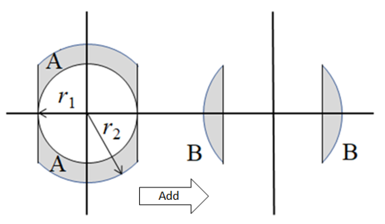
3.1. Improved Model

The second section gave the two-dimensional vibration model. When comparing the equivalent stiffness values calculated by the two-dimensional theoretical vibration model with the equivalent stiffnesses calculated based on numerical values, it was found that when the coating material was rubber, the calculation results of the two-dimensional theoretical vibration model were lower than the results of numerical calculations, which was due to the underestimation of the equivalent stiffness of the soft coating; moreover, component B was not considered, which may have had an impact on the results. Through simple analysis, it can be found that when the soft coating in region B vibrates left and right, it undergoes shear deformation and provides a certain degree of rigidity. The shear stiffness of the B component can affect the elastic properties of the metamaterial concrete, which modulates the frequency of the single cell and thus the formation and nature of the bandgap of the metamaterial concrete. Therefore, in the improved two-dimensional vibration theory model, the stiffness of this part is included in the calculation of the equivalent stiffness of the soft coating, to achieve an overall equivalent stiffness value that is closer to the real situation.

As shown in Figure 7, the equivalent stiffness k of the soft coating in area A is calculated according to Formula (25), denoted as $k_a$, and the equivalent stiffness $k_b$ of the soft coating in area B can be expressed as

$$k_b=\frac{2\times G\times \sqrt{r_2^2-r_1^2}+r_2\arccos \left(r_1/r_2\right)}{r_2-r_1}$$

(28)

Then, the overall equivalent stiffness k is

$$k=k_a+k_b$$

(29)

According to the material parameters in Table 2 and the geometric dimensions in Table 1, the equivalent stiffness of the aggregate of the improved two-dimensional vibration theory model can be calculated by Formula (29). In order to compare the improved two-dimensional vibration theory model with the first two models, the prediction results of the three models and the calculation results of numerical simulation are also listed in

Table 4. Comparison of the improved two-dimensional model and numerical simulation results.

Coating	Equivalent Stiffness (103 kN/m)
	Numerical Simulation	One- Dimensional Model	Error Rate (%)	Two-Dimensional Model	Error Rate (%)	Improved Two-Dimensional Model	Error Rate (%)
1 mm Rubber	19.41	3.84	−80.22	17.91	−7.73	18.58	−4.28
2 mm Rubber	8.59	1.68	−80.44	8.08	−5.94	8.55	−0.47
3 mm Rubber	4.80	0.96	−80.00	4.75	−1.04	5.13	6.88

.

It can be seen from Table 4 that for the metamaterial concrete unit cell whose coating material is rubber, the equivalent stiffness calculated by the improved two-dimensional vibration theory model is greater than the equivalent stiffness calculated by numerical simulation. When the coating thicknesses are at 1 mm, 2 mm and 3 mm, the error rates between the equivalent stiffness calculated by the two-dimensional vibration theory model and the equivalent stiffness calculated by numerical simulation are −4.28%, −0.47% and 6.88%, respectively. When the coating thickness is small, the error rate of the improved two-dimensional model is negative, and the error rate of the improved two-dimensional model decreases with the increase in Poisson’s ratio; when the coating thickness is large, the error rate of the improved two-dimensional model becomes positive. The reason for the above phenomenon is that when the thickness of the coating material increases, the shear action considered by the improved two-dimensional theoretical model is less likely to occur, and the force required for shearing motion is greater, resulting in the predicted values of the improved two-dimensional theoretical model becoming greater than the numerical simulation results.

3.2. Parameter Analysis

In the previous section, the one-dimensional theoretical vibration model, the two-dimensional model and the improved two-dimensional model for calculating the equivalent stiffness value of the metamaterial concrete unit cell were given, respectively. When comparing the equivalent stiffness values calculated by the theoretical models and the equivalent stiffness values of the numerical simulation, it could be seen that the size of the resonant aggregate and the material parameters of the coating material affected the error rates of the three theoretical vibration models. In order to further determine the application range of the different theoretical vibration models, this section comprehensively analyzes the prediction results and error rates of the three models under different resonant aggregate sizes and coating material parameters. This section is divided into three working conditions, namely working condition 1 ($r_2$ = 9 mm, t = 1 mm), working condition 2 ($r_2$ = 8 mm, t = 2 mm) and working condition 3 ($r_2$ = 7 mm, t = 3 mm). The elastic modulus and Poisson’s ratio of the soft coating were changed under each working condition. The elastic moduli G of the coating were 3 × 10⁻⁵ GPa, 3 × 10⁻⁴ GPa, 3 × 10⁻³ GPa and 3 × 10⁻² GPa. The one-dimensional model, two-dimensional model and improved two-dimensional model were used to calculate the theoretical solutions under various working conditions, and the error rates between the calculation results and the numerical simulation results were calculated.

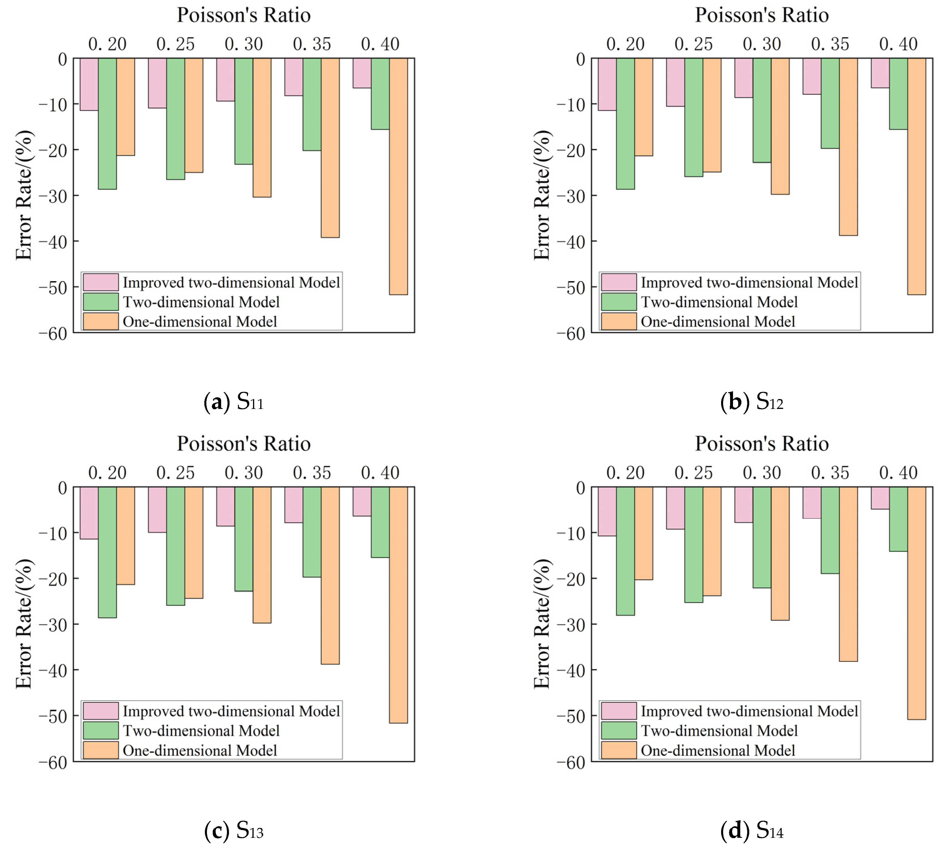
3.2.1. Working Condition 1

Table 5. Comparison of the improved two-dimensional theoretical vibration model and numerical simulation results in working condition 1.

Parameters		Equivalent Stiffness (103 kN/m)
S	$\mathit{\nu }$	Numerical Simulation	One- Dimensional	Error Rate (%)	Two- Dimensional	Error Rate (%)	Improved Two- Dimensional	Error Rate (%)
S11	0.20	1.22	0.96	−21.31	0.87	−28.69	1.08	−11.48
	0.25	1.28		−25.00	0.94	−26.56	1.14	−10.94
	0.30	1.38		−30.43	1.06	−23.19	1.25	−9.42
	0.35	1.58		−39.24	1.26	−20.25	1.45	−8.22
	0.40	1.99		−51.76	1.68	−15.58	1.86	−6.53
S12	0.20	12.21	9.60	−21.38	8.71	−28.67	10.81	−11.47
	0.25	12.78		−24.88	9.41	−25.91	11.43	−10.56
	0.30	13.68		−29.82	10.56	−22.81	12.50	−8.63
	0.35	15.69		−38.81	12.59	−19.76	14.45	−7.90
	0.40	19.90		−51.75	16.81	−15.57	18.61	−6.48
S13	0.20	122.14	96.00	−21.40	87.14	−28.66	108.15	−11.45
	0.25	126.98		−24.39	94.11	−25.89	114.28	−10.00
	0.30	136.75		−29.80	105.57	−22.80	124.97	−8.61
	0.35	156.86		−38.80	125.87	−19.76	144.55	−7.85
	0.40	198.76		−51.70	168.05	−15.45	186.07	−6.38
S14	0.20	1205.01	960.00	−20.33	871.39	−28.11	1081.54	−10.78
	0.25	1259.84		−23.80	941.10	−25.30	1142.84	−9.29
	0.30	1355.93		−29.20	1055.72	−22.14	1249.71	−7.83
	0.35	1553.40		−38.20	1258.67	−18.97	1445.47	−6.95
	0.40	1955.99		−50.92	1680.53	−14.08	1860.66	−4.87

shows the law of numerical simulation results changing with coating elastic modulus and Poisson’s ratio when $r_2$ = 9 mm and t = 1 mm, and the prediction results of the three theoretical models and their error rates compared to the numerical simulation results. S₁₁, S₁₂, S₁₃ and S₁₄ in the Table 5 represent the models where the elastic modulI were 3 × 10⁻⁵ GPa, 3 × 10⁻⁴ GPa, 3 × 10⁻³ GPa and 3 × 10⁻² GPa, respectively. The positive and negative values of the error rate indicate that the theoretical result was smaller than or greater than the numerical simulation result, respectively.

It can be seen from Table 5 and Figure 8 and Figure 9 that when the elastic modulus of the coating is constant, an increase in Poisson’s ratio leads to more lateral expansion during stress, which increases the effective stiffness of the surface, and the equivalent stiffness value obtained by numerical simulation increases with the increase in Poisson’s ratio. In contrast, the one-dimensional model may not be able to take into account this lateral expansion effect, so the prediction results of the one-dimensional theoretical model remain unchanged. The one-dimensional model assumes that the deformation of the material occurs in only one direction, ignoring the lateral expansion effect of the surface, and, therefore, fails to capture the effect of increasing Poisson’s ratio on the surface stiffness. Taking S₁₁ as an example, when Poisson’s ratio increases from 0.20 to 0.40, the error rate of the one-dimensional theoretical model increases from −21.31% to −51.76%. When the elastic modulus is constant, the prediction result of the two-dimensional theoretical model increases with the increase in Poisson’s ratio, so the error rate of the two-dimensional model decreases with the increase in Poisson’s ratio. Taking S₁₁ as an example, when Poisson’s ratio increases from 0.20 to 0.40, the error rate of the two-dimensional theoretical model decreases from −28.69% to −15.58%. When the elastic modulus is constant, the prediction results of the improved two-dimensional theoretical model increase with the increase in Poisson’s ratio. Taking S₁₁ as an example, when Poisson’s ratio increases from 0.20 to 0.40, the error rate of the improved two-dimensional theoretical model changes from negative to positive, from −11.48% to 6.53%. This lateral expansion effect may be better accounted for in the improved two-dimensional theoretical model as Poisson’s ratio increases due to the model’s more comprehensive consideration of the deformation properties of the coating material.

It can be seen from Table 5 and Figure 10 and Figure 11 that when Poisson’s ratio is constant, the equivalent stiffness value obtained by numerical simulation increases. The prediction result of the one-dimensional theoretical model increases with the increase in the elastic modulus, and the error rate of the one-dimensional theoretical model decreases with the increase in the elastic modulus. Taking a Poisson’s ratio of 0.25 as an example, when the elastic modulus increases from 3 × 10⁻⁵ GPa to 3 × 10⁻² GPa, the error rate of the one-dimensional theoretical model decreases from −25.00% to 23.80%. When Poisson’s ratio is constant, the prediction results of the two-dimensional theoretical model increase with the increase in the elastic modulus, and the error rate of the two-dimensional model decreases with the increase in the elastic modulus. Taking Poisson’s ratio of 0.25 as an example, when the elastic modulus increases from 3 × 10⁻⁵ GPa to 3 × 10⁻² GPa, the error rate of the two-dimensional theoretical model decreases from −26.56% to −25.30%. When Poisson’s ratio is constant, the prediction result of the improved two-dimensional theoretical model increases with the increase in the elastic modulus, and the error rate of the improved two-dimensional model decreases with the increase in the elastic modulus. Taking a Poisson’s ratio of 0.25 as an example, when the elastic modulus increases from 3 × 10⁻⁵ GPa to 3 × 10⁻² GPa, the error rate of the improved two-dimensional theoretical model decreases from −10.94% to −9.29%. The error rate of the improved two-dimensional model in working condition 1 is generally within 10%, and the error rate of the improved two-dimensional theoretical model is much lower than the error rates of the one- and two-dimensional models. The improved two-dimensional model shows significant advantages in terms of prediction error rate, especially under operating condition 1, where the error rate usually stays within 10%, which is much lower than that of the one- and two-dimensional theoretical models.

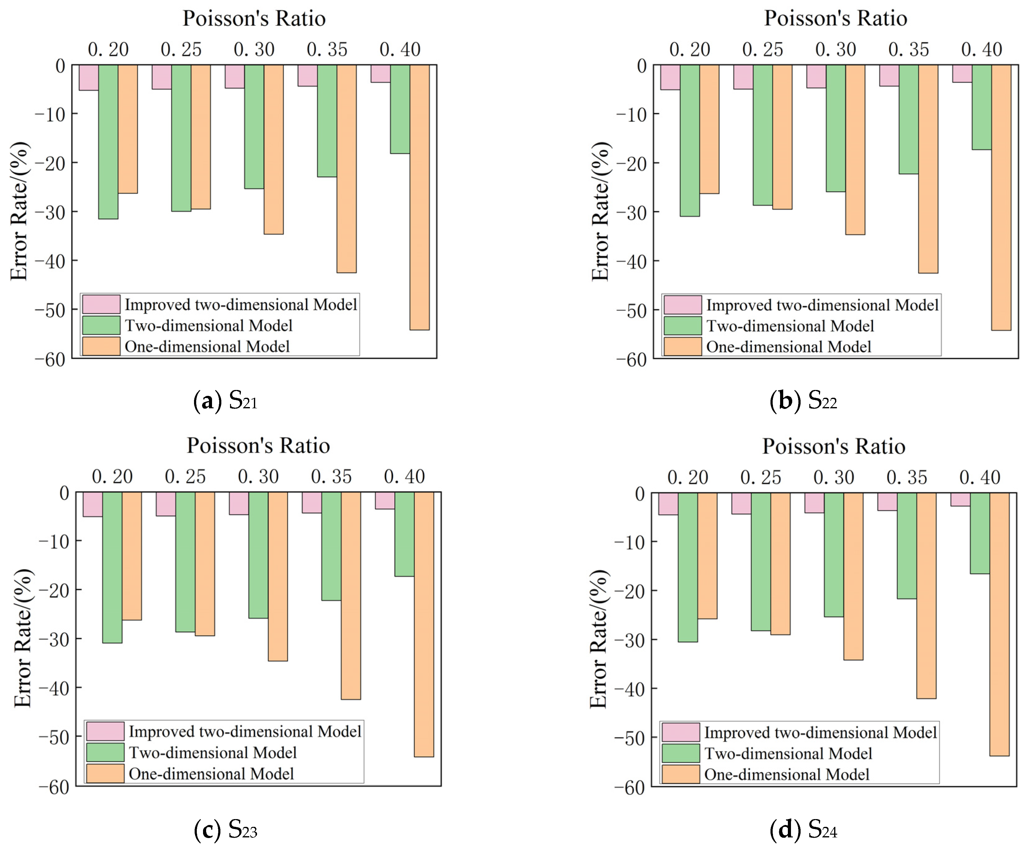
3.2.2. Working Condition 2

Table 6. Comparison of the improved two-dimensional theoretical vibration model and numerical simulation results in working condition 2.

Parameters		Equivalent Stiffness (103 kN/m)
S	$\mathit{\nu }$	Numerical Simulation	One- Dimensional	Error Rate (%)	Two- Dimensional	Error Rate (%)	Improved Two- Dimensional	Error Rate (%)
S21	0.20	0.570	0.42	−26.32	0.393	−31.58	0.540	−5.26
	0.25	0.596		−29.53	0.425	−30.00	0.566	−5.03
	0.30	0.643		−34.68	0.476	−25.35	0.612	−4.82
	0.35	0.731		−42.55	0.568	−22.97	0.699	−4.42
	0.40	0.918		−54.25	0.759	−18.21	0.885	−3.63
S22	0.20	5.699	4.20	−26.30	3.932	−31.00	5.404	−5.17
	0.25	5.959		−29.52	4.247	−28.73	5.660	−5.02
	0.30	6.431		−34.69	4.764	−25.92	6.123	−4.80
	0.35	7.311		−42.55	5.680	−22.31	6.988	−4.42
	0.40	9.178		−54.24	7.584	−17.38	8.845	−3.63
S23	0.20	56.95	42.00	−26.25	39.32	−30.96	54.04	−5.11
	0.25	59.56		−29.48	42.47	−28.69	56.60	−4.97
	0.30	64.27		−34.65	47.64	−25.88	61.26	−4.68
	0.35	73.06		−42.51	56.80	−22.26	69.88	−4.35
	0.40	91.71		−54.20	75.83	−17.32	88.45	−3.55
S24	0.20	566.15	420.00	−25.81	393.22	−30.54	540.40	−4.55
	0.25	591.98		−29.05	424.68	−28.26	565.97	−4.39
	0.30	638.71		−34.24	476.41	−25.41	612.26	−4.14
	0.35	725.61		−42.12	567.99	−21.72	698.81	−3.69
	0.40	909.55		−53.82	758.36	−16.62	884.51	−2.75

Note: Since the values of S₂₁ and S₂₂ are relatively small, three decimal places are reserved.

shows the law of the numerical simulation results changing with the elastic modulus and Poisson’s ratio of the coating when $r_2$ = 9 mm and t = 2 mm, as well as the prediction results of the three theoretical models and their error rates with the numerical simulation results. S₂₁, S₂₂, S₂₃ and S₂₄ in the Table 6 represent the models where the elastic moduli are 3 × 10⁻⁵ GPa, 3 × 10⁻⁴ GPa, 3 × 10⁻³ GPa and 3 × 10⁻² GPa, respectively. The positive and negative values of the error rate indicate that the theoretical result is smaller than or greater than the numerical simulation result, respectively.

Comparing Table 5 and Table 6, it can be found that when the elastic modulus and Poisson’s ratio are determined, the prediction results of the one-dimensional theoretical model decrease with the increase in coating thickness t, while the error rate increases with the increase in coating thickness t. Taking the elastic modulus of 3 × 10⁻² GPa and Poisson’s ratio of 0.25 as an example, when the thickness of the coating increases from 1 mm to 2 mm, the error rate of the one-dimensional model increases from −23.80% to −29.05%. The one-dimensional model simplifies the coating thickness variation by treating it as a uniform layer throughout the structure. As the coating thickness increases, this simplification becomes less accurate, leading to decreased prediction results and increased error rates. When the elastic modulus and Poisson’s ratio are determined, the prediction results of the two-dimensional theoretical model decrease with the increase in coating thickness t, while the error rate increases with the increase in coating thickness t. Taking the elastic modulus of 3 × 10⁻² GPa and Poisson’s ratio of 0.25 as an example, when the coating thickness increases from 1 mm to 2 mm, the error rate of the two-dimensional model increases from −25.30% to −28.26%. The reason for the above phenomenon is that the two-dimensional model simplifies the mechanical behavior of the coating by neglecting certain deformation modes, such as shear deformation, which become more significant as the coating thickness increases. This simplification contributes to larger errors in predicting mechanical behavior, particularly in regions with thicker coatings. When the elastic modulus and Poisson’s ratio are determined, the prediction results of the improved two-dimensional theoretical model decrease with the increase in coating thickness t, while the error rate decreases with the increase in coating thickness t. Taking the elastic modulus of 3 × 10⁻² GPa and Poisson’s ratio of 0.25 as an example, when the coating thickness increases from 1 mm to 2 mm, the error rate of the two-dimensional model decreases from −9.29% to −4.39%. Compared to the two-dimensional model, the improved model addresses limitations such as neglecting shear deformation, resulting in decreased error rates, particularly in regions with thicker coatings. In working condition 2, the error rate of the improved two-dimensional model is generally within 5%, and the error rate of the improved two-dimensional theoretical model is much lower than the error rates of the one- and two-dimensional theoretical models.

From Table 6 and Figure 12 and Figure 13, it can be seen that when the geometric conditions are determined, the predicted change laws of the three models are basically consistent with those of working condition 1 ($r_2$ = 9 mm, t = 1 mm). That is, when the elastic modulus of the coating is constant, the equivalent stiffness value obtained by numerical simulation increases with the increase in Poisson’s ratio; the prediction result of the one-dimensional theoretical model remains unchanged, so the error rate of the one-dimensional theoretical model increases with the increase in Poisson’s ratio. Taking S₂₁ as an example, when Poisson’s ratios are 0.20, 0.25, 0.30, 0.35 and 0.40, the error rates of the one-dimensional theoretical model are −26.32%, −29.53%, −34.68%, −42.55% and −54.25%, respectively.

It can be seen from Table 6 and Figure 14 and Figure 15 that when the elastic modulus is constant, the prediction result of the two-dimensional theoretical model increases with the increase in Poisson’s ratio, so the error rate of the two-dimensional model decreases with the increase in Poisson’s ratio. Taking S₂₁ as an example, when Poisson’s ratios are 0.20, 0.25, 0.30, 0.35 and 0.40, the error rates of the two-dimensional theoretical model are −31.58%, −30.00%, −25.35%, −22.97% and −18.21%, respectively. When the elastic modulus is constant, the prediction result of the improved two-dimensional theoretical model increases with the increase in Poisson’s ratio, so the error rate of the improved two-dimensional model decreases with the increase in Poisson’s ratio. Taking S₂₁ as an example, when Poisson’s ratios are 0.20, 0.25, 0.30, 0.35 and 0.40, the error rates of the improved two-dimensional theoretical model are −5.26%, −5.03%, −4.82%, −4.42% and −3.63%, respectively. When Poisson’s ratio is constant, the equivalent stiffness value obtained by numerical simulation increases with the increase in the elastic modulus, while the prediction result of the one-dimensional theoretical model increases and its error rate decreases. Taking Poisson’s ratio of 0.25 as an example, when the elastic modulus increases from 3 × 10⁻⁵ GPa to 3 × 10⁻² GPa, the error rate of the one-dimensional theoretical model decreases from −29.53% to −29.05%. When Poisson’s ratio is constant, the prediction results of the two-dimensional theoretical model increase with the increase in the elastic modulus, while the error rate of the two-dimensional model decreases. Taking Poisson’s ratio of 0.25 as an example, when the elastic modulus increases from 3 × 10⁻⁵ GPa to 3 × 10⁻² GPa, the error rate of the two-dimensional theoretical model decreases from −30.00% to −28.26%. When Poisson’s ratio is constant, the prediction result of the improved two-dimensional theoretical model increases with the increase in the elastic modulus, while the error rate of the improved two-dimensional model decreases. Taking Poisson’s ratio of 0.25 as an example, when the elastic modulus increases from 3 × 10⁻⁵ GPa to 3 × 10⁻² GPa, the error rate of the improved two-dimensional theoretical model decreases from −5.03% to −4.39%.

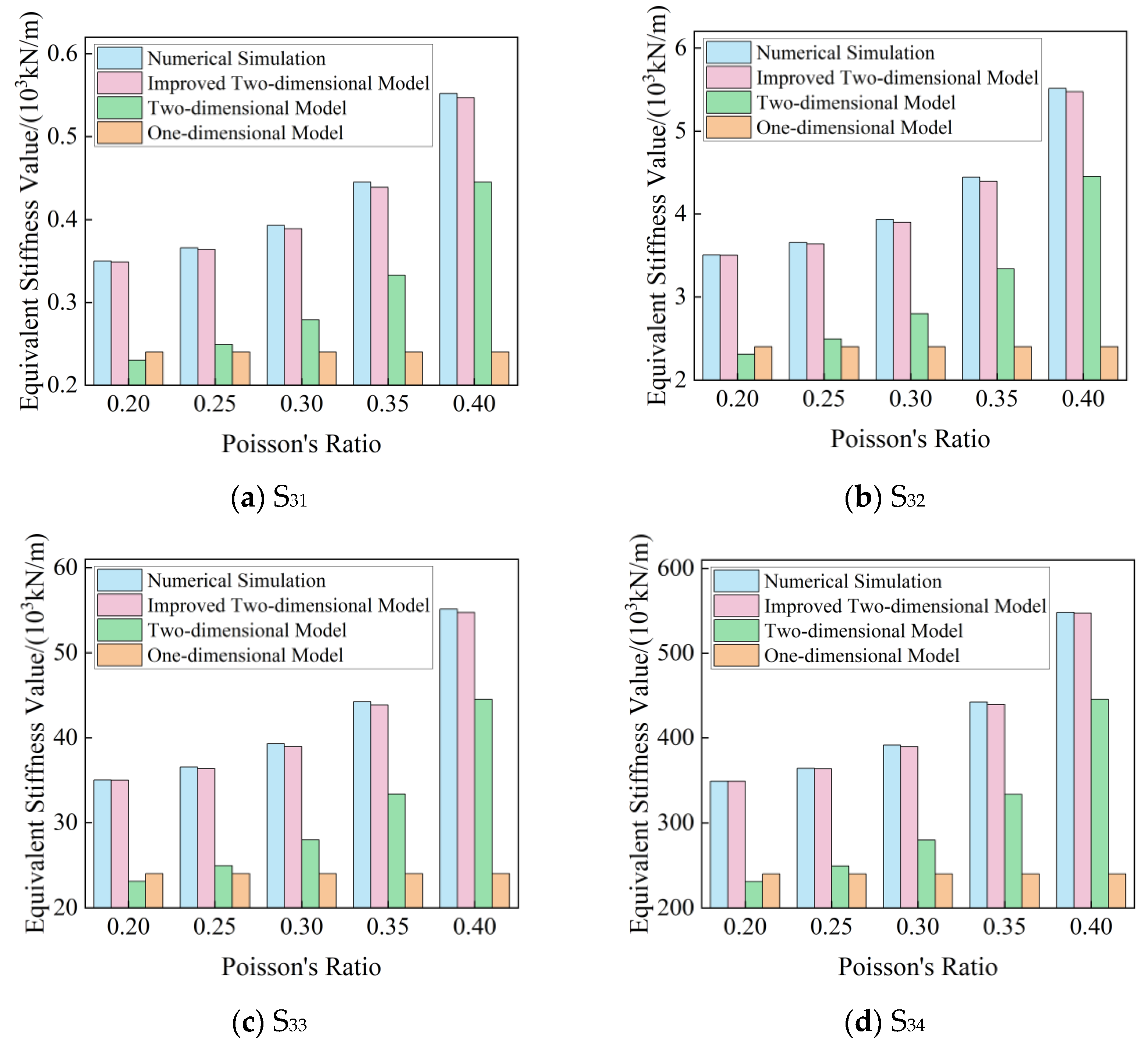
3.2.3. Working Condition 3

Table 7. Comparison of the improved two-dimensional theoretical vibration model and numerical simulation results in working condition 3.

Parameters		Equivalent Stiffness (103 kN/m)
S	$\mathit{\nu }$	Numerical Simulation	One- Dimensional	Error Rate (%)	Two- Dimensional	Error Rate (%)	Improved Two- Dimensional	Error Rate (%)
S31	0.20	0.350	0.24	−31.51	0.230	−34.28	0.349	−0.14
	0.25	0.366		−34.36	0.249	−31.97	0.364	−0.55
	0.30	0.393		−38.97	0.279	−29.01	0.389	−1.02
	0.35	0.445		−46.01	0.333	−25.27	0.439	−1.15
	0.40	0.552		−56.49	0.445	−19.38	0.547	−0.75
S32	0.20	3.504	2.40	−31.51	2.310	−34.08	3.500	−0.11
	0.25	3.656		−34.36	2.494	−31.78	3.636	−0.55
	0.30	3.933		−38.97	2.798	−28.86	3.897	−0.92
	0.35	4.445		−46.01	3.336	−24.95	4.394	−1.15
	0.40	5.515		−56.49	4.454	−19.24	5.474	−0.74
S33	0.20	35.03	24.00	−31.49	23.10	−34.06	35.00	−0.09
	0.25	36.55		−34.34	24.94	−31.76	36.37	−0.49
	0.30	39.31		−38.95	27.98	−28.82	38.97	−0.86
	0.35	44.28		−45.80	33.36	−24.66	43.89	−0.88
	0.40	55.12		−56.46	44.54	−19.19	54.74	−0.69
S34	0.20	348.91	240.00	−31.21	230.97	−33.80	348.89	−0.01
	0.25	364.02		−34.07	249.45	−31.47	363.67	−0.10
	0.30	391.46		−38.69	279.83	−28.52	389.66	−0.46
	0.35	442.24		−45.73	333.63	−24.56	439.39	−0.64
	0.40	548.21		−56.22	445.45	−18.74	547.43	−0.14

Note: Since the values of S₃₁ and S₃₂ are relatively small, three decimal places are reserved.

shows the law of numerical simulation results changing with the coating elastic modulus and Poisson’s ratio when $r_2$ = 9 mm and t = 3 mm, as well as the prediction results of the three theoretical models and their error rates compared to the numerical simulation results. S₃₁, S₃₂, S₃₃ and S₃₄ in the Table 7 represent models where the elastic moduli are 3 × 10⁻⁵ GPa, 3 × 10⁻⁴ GPa, 3 × 10⁻³ GPa and 3 × 10⁻² GPa, respectively. The positive and negative values of the error rate indicate that the theoretical result was smaller than or greater than the numerical simulation result, respectively.

When comparing Table 5, Table 6 and Table 7, it can be found that when the elastic modulus and Poisson’s ratio are determined, the prediction results of the one-dimensional theoretical model decrease with the increase in coating thickness t, while the error rate increases t. Taking the elastic modulus of 3 × 10⁻² GPa and Poisson’s ratio of 0.25 as an example, when the coating thicknesses are 1 mm, 2 mm and 3 mm, the error rates of the one-dimensional model are −23.80%, −29.05% and −34.07%. Consistent with the analysis in Section 3.2.2, the reason for the above phenomenon is that when the coating thickness is small (1 mm), the thickness difference between the coating at the center and the coating at both ends is small. According to the one-dimensional theoretical model, it is relatively reasonable to simplify the coating to a round rod with equal thickness. When the elastic modulus and Poisson’s ratio are determined, the prediction results of the two-dimensional theoretical model decrease with the increase in coating thickness t, while the error rate increases. Taking the elastic modulus of 3 × 10⁻² GPa and Poisson’s ratio of 0.25 as an example, when the coating thicknesses are 1 mm, 2 mm and 3 mm, the error rates of the two-dimensional model are −25.30%, −28.26% and −31.47%. When the elastic modulus and Poisson’s ratio are determined, the prediction results of the improved two-dimensional theoretical model decrease with the increase in coating thickness t, while the error rate decreases. Taking the elastic modulus of 3 × 10⁻² GPa and Poisson’s ratio of 0.25 as an example, when the coating thicknesses are 1 mm, 2 mm and 3 mm, the error rates of the improved two-dimensional model are −9.29%, −4.39% and −0.10%, respectively. In working condition 3, the error rate of the improved two-dimensional model is generally within 1%, and the error rate of the improved two-dimensional theoretical model is much lower than the error rates of the one- and two-dimensional theoretical models.

From Table 7 and Figure 16 and Figure 17, it can be seen that when the geometric conditions are determined, the predicted change laws of the three models are basically consistent with those of working condition 1 ($r_2$ = 9 mm, t = 1 mm) and working condition 2 ($r_2$ = 9 mm, t = 2 mm). That is, when the elastic modulus of the coating is constant, the equivalent stiffness value obtained by numerical simulation increases with the increase in Poisson’s ratio. The prediction result of the one-dimensional theoretical model remains unchanged, so the error rate of the one-dimensional theoretical model increases with the increase in Poisson’s ratio.

It can be seen from Table 7 and Figure 18 and Figure 19 that when the elastic modulus is constant, the prediction result of the two-dimensional theoretical model increases with the increase in Poisson’s ratio, so the error rate of the two-dimensional model decreases. When the elastic modulus is constant, the prediction results of the improved two-dimensional theoretical model increase with the increase in Poisson’s ratio. The two-dimensional model is able to capture the additional deformation associated with transverse strains. Higher Poisson’s ratios indicate a greater tendency for transverse expansion or contraction under loading, which can be more accurately accounted for by the two-dimensional model than the one-dimensional model. When Poisson’s ratio is constant, the equivalent stiffness value obtained by numerical simulation increases; meanwhile, the prediction result of the one-dimensional theoretical model increases with the increase in the elastic modulus, while its error rate decreases. When Poisson’s ratio is constant, the prediction results of the two-dimensional theoretical model increase with the increase in the elastic modulus, while the error rate of the two-dimensional model decreases. When Poisson’s ratio is constant, the prediction result of the improved two-dimensional theoretical model increases with the increase in the elastic modulus, while the error rate of the improved two-dimensional model decreases. The improved two-dimensional model takes into account the shear behavior in the material when modeling, rather than being limited to considering only its tensile and compressive properties. Meanwhile, the two-dimensional model usually assumes that the material will only deform orthogonally, ignoring shear deformation. However, in some cases, especially when the material is subjected to complex loading, shear deformation can have a significant effect on the behavior of the structure.

4. Discussion

Through the above study, we found that the values of the newly proposed two-dimensional model were closest to the numerical simulation results, with the smallest error rates under various working conditions. The model was compared with the theoretical model of metamaterial concrete monoclonal cells proposed by Yingjie Gao [43] in a concrete wave-absorbing plate,. The model proposed by Yingjie Gao takes into account the influence of the soft-coated circular material on the basis of a one-dimensional model, and multiplies the perimeter π on the basis of the formula of that model. From Table 5, Table 6 and Table 7, it can be seen that, when the results of the one-dimensional model are multiplied by the perimeter π, the value of the model will be much larger than the results of the numerical simulation, and the corresponding error rate will be much higher than that of the improved two-dimensional model.

Bandgap is an important property of metamaterials, which refers to the specific blocking effect of metamaterials on the propagation of electromagnetic or mechanical waves in a specific frequency range. Introducing metamaterial structures with bandgap properties into concrete can give concrete new functions, such as vibration isolation.

The study of bandgap characteristics enables us to obtain the parameters and laws affecting the bandgap value of metamaterial concrete, which guides the application of metamaterial concrete in practical vibration isolation projects. The calculation of theoretical formulas helps us to better understand the vibration mode and vibration mechanism of the monoclonal cell of metamaterial concrete and its energy absorption and vibration isolation mechanism. Equivalent stiffness, as one of the important quantities in the bandgap calculation formula, is of great significance in determining the geometric dimensions and material parameters of the metamaterial concrete’s single cell. In actual projects such as subway and underpass tunnels, its vibration frequency is relatively fixed, within a range, and the vibration frequency that needs to be blocked is the target bandgap. The accurate calculation of the formula can be obtained from the concrete cell of metamaterials and parameter optimization to achieve the safety, economy and efficiency of the project.

Other influences on the equivalent stiffness of metamaterial concrete’s unit cell deserve to be discussed. Equivalent mass is one of the important quantities affecting the bandgap of metamaterial concrete, so it is also necessary to derive the effective mass formula accurately. Meanwhile, the model in this paper only includes a single aggregate, and the bandgap characteristics and corresponding theoretical formulas for multiple aggregates, such as double-cladding and multi-cladding metamaterial concretes, have not yet been investigated. In addition, aggregate shape is also a point of interest, which can be optimized using computer technology. The above will be studied in subsequent work.

5. Conclusions

Based on the existing one- and two-dimensional theoretical vibration models, an improved two-dimensional theoretical vibration model has been proposed, and finite element simulation has been carried out to analyze the influence of different parameters on its equivalent stiffness. The following conclusions are drawn:

(1)

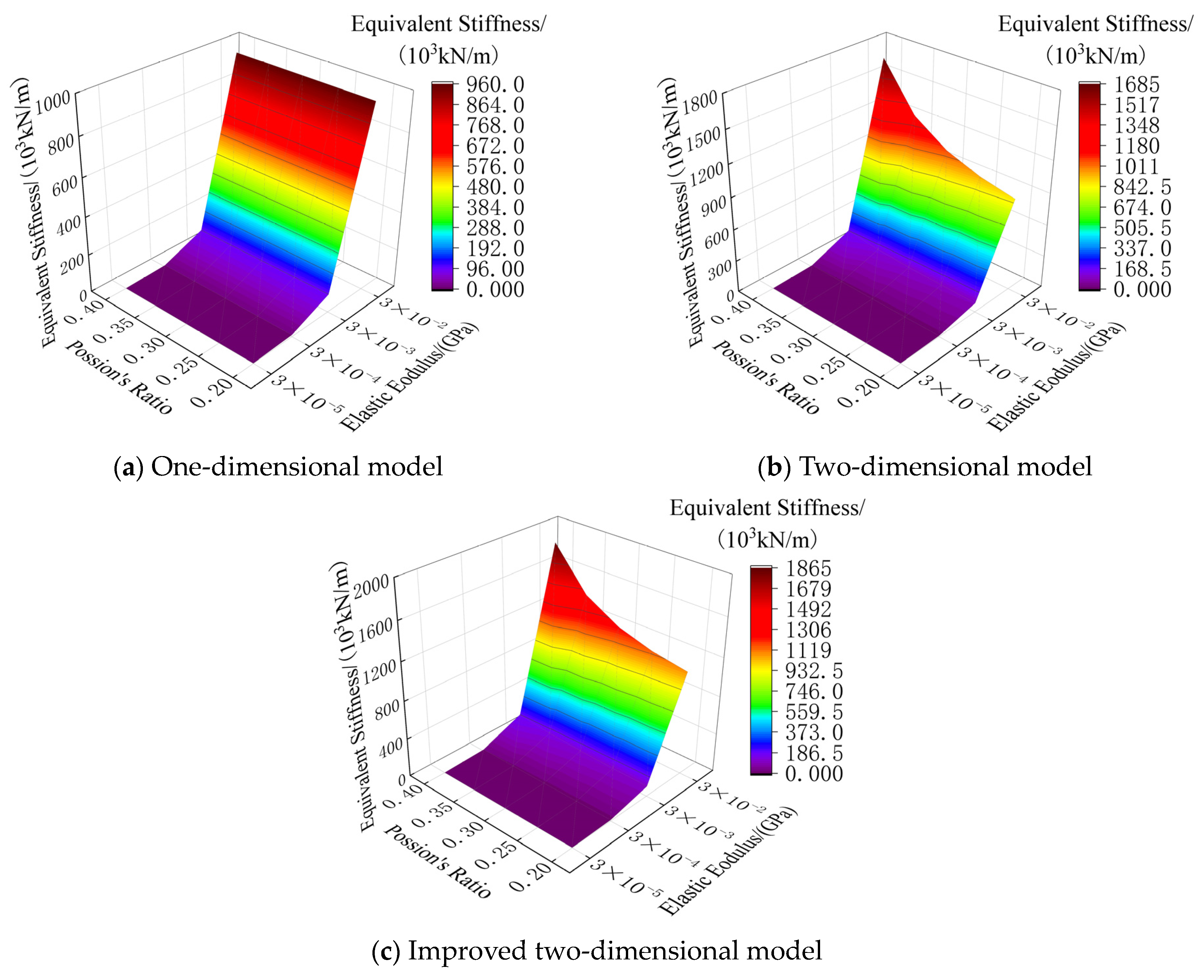
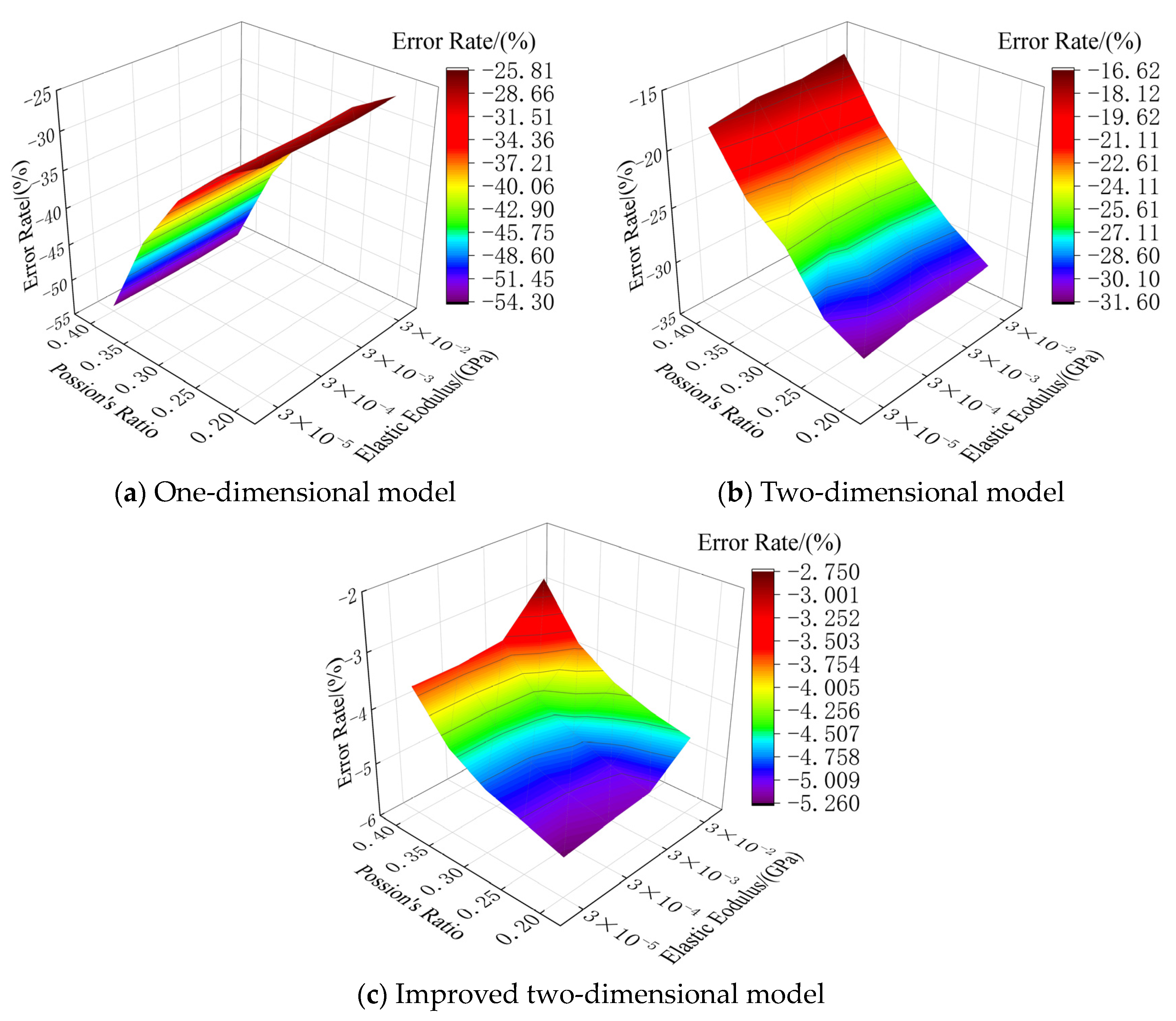
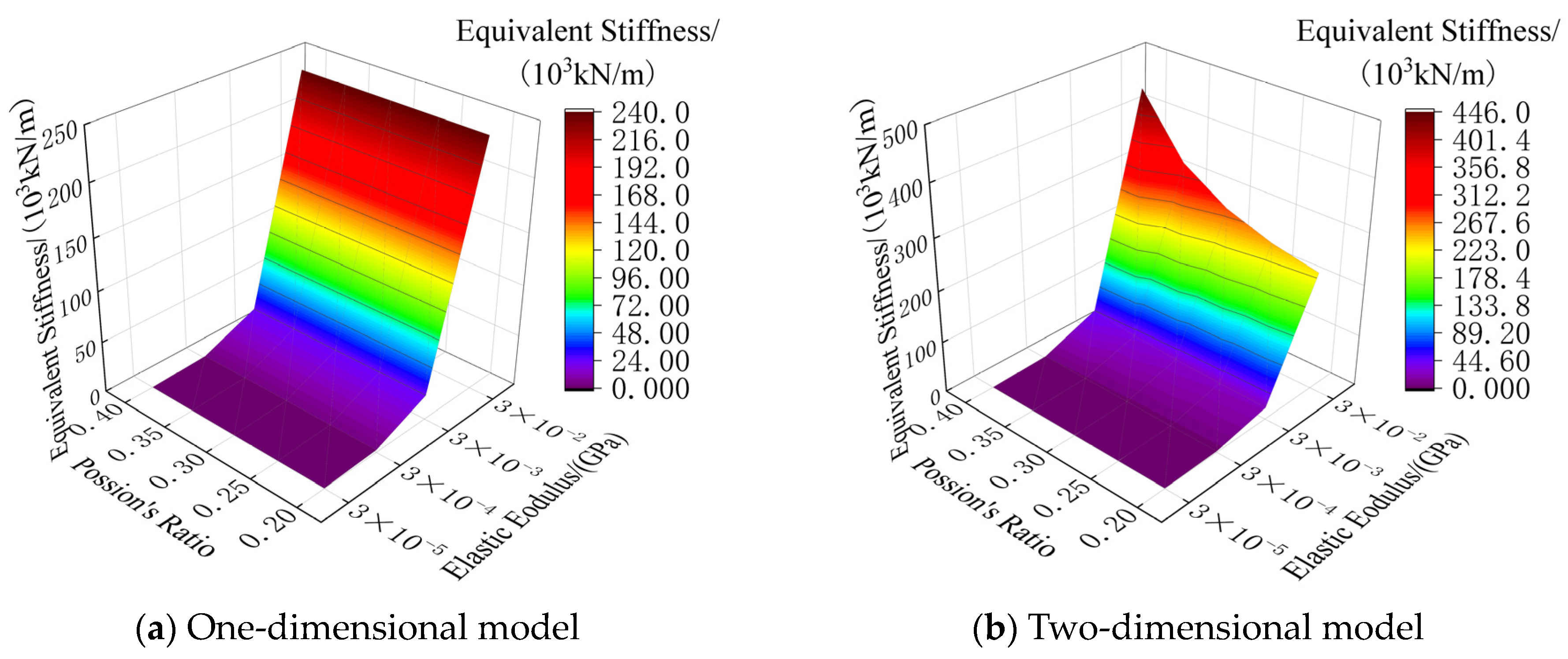
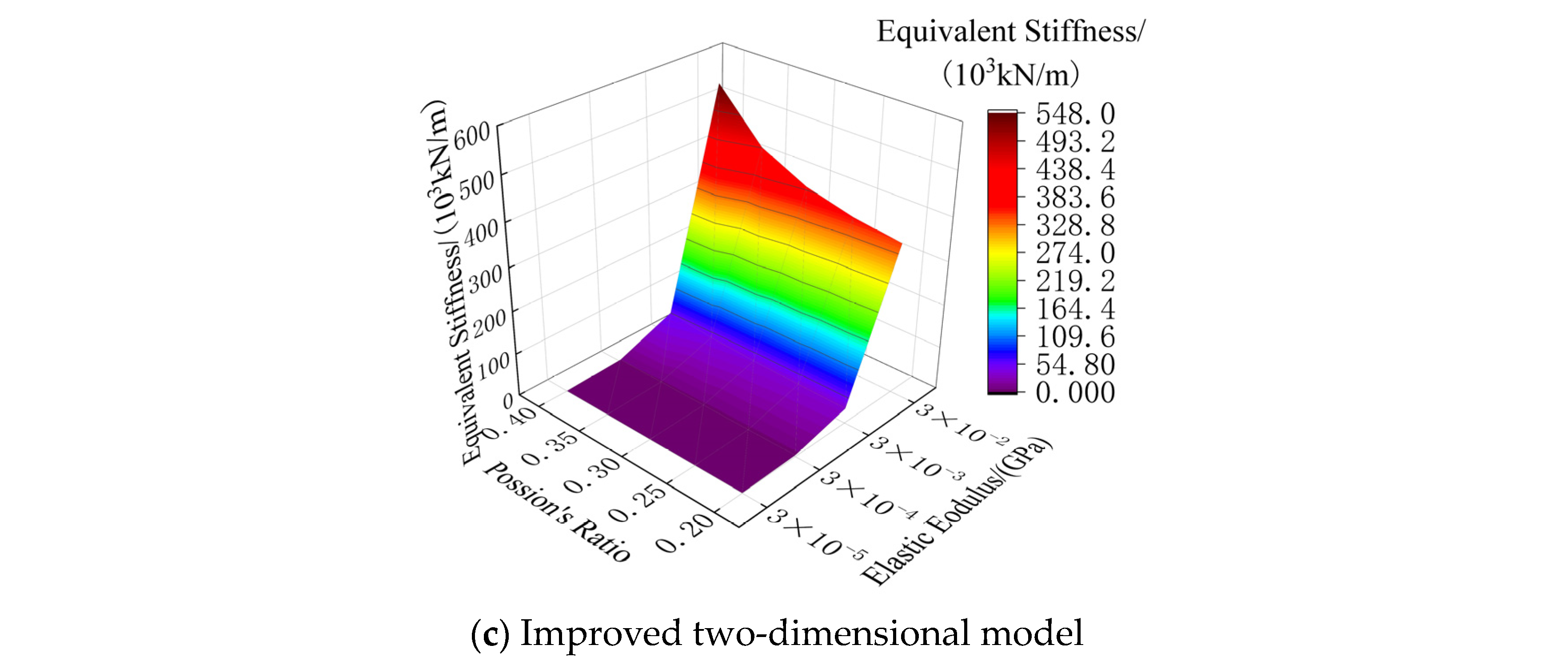
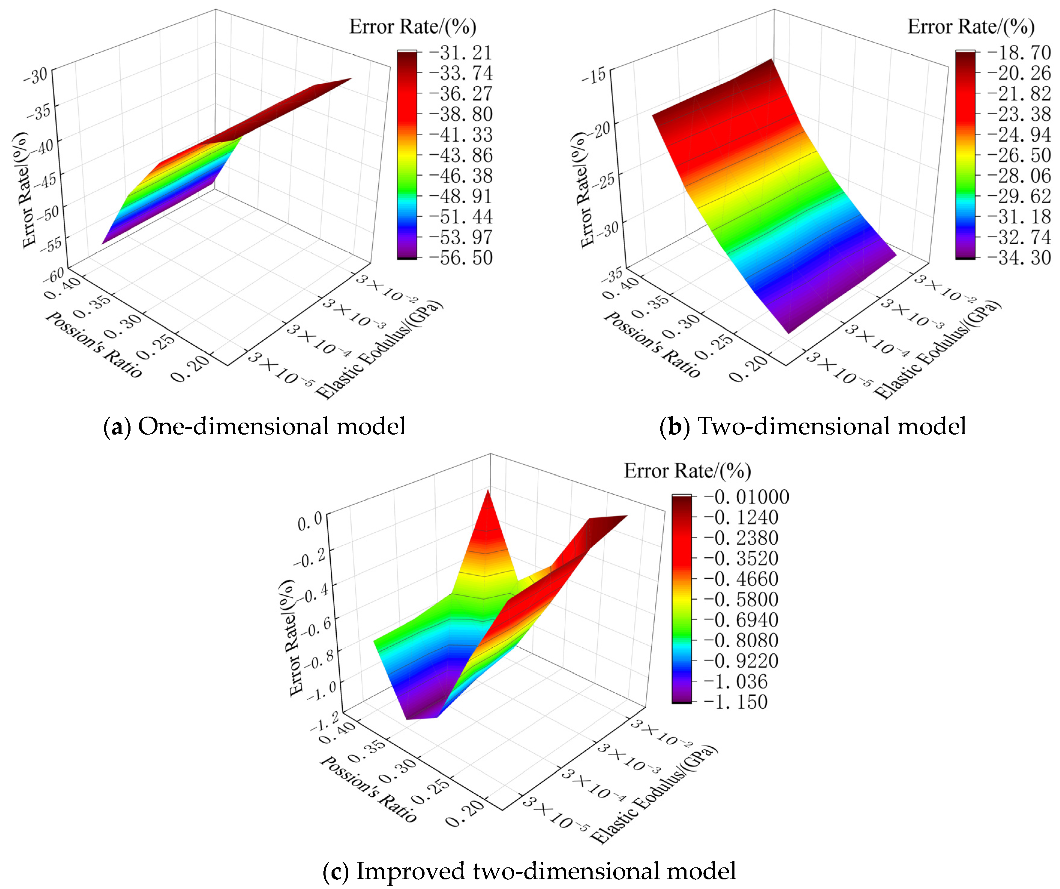
When the elastic modulus and Poisson’s ratio are constant, the prediction results of the one- and two-dimensional theoretical vibration models and the improved two-dimensional model all decrease with the increase in the coating thickness, while the error rates increase. When the geometric parameters and Poisson’s ratio are constant, the prediction results of the one-and two-dimensional theoretical vibration models and the improved two-dimensional model increase with the increase in the elastic modulus, while the error rates decrease.

(2)

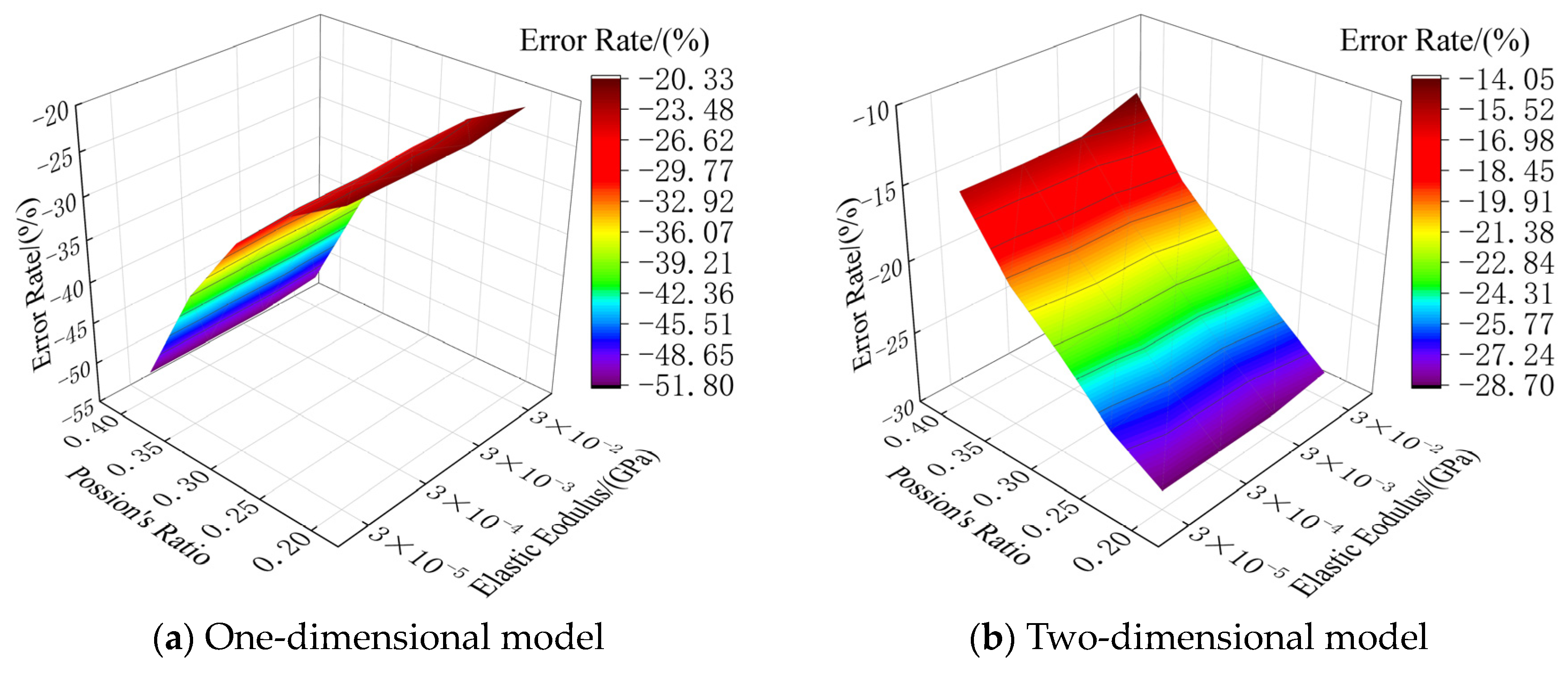
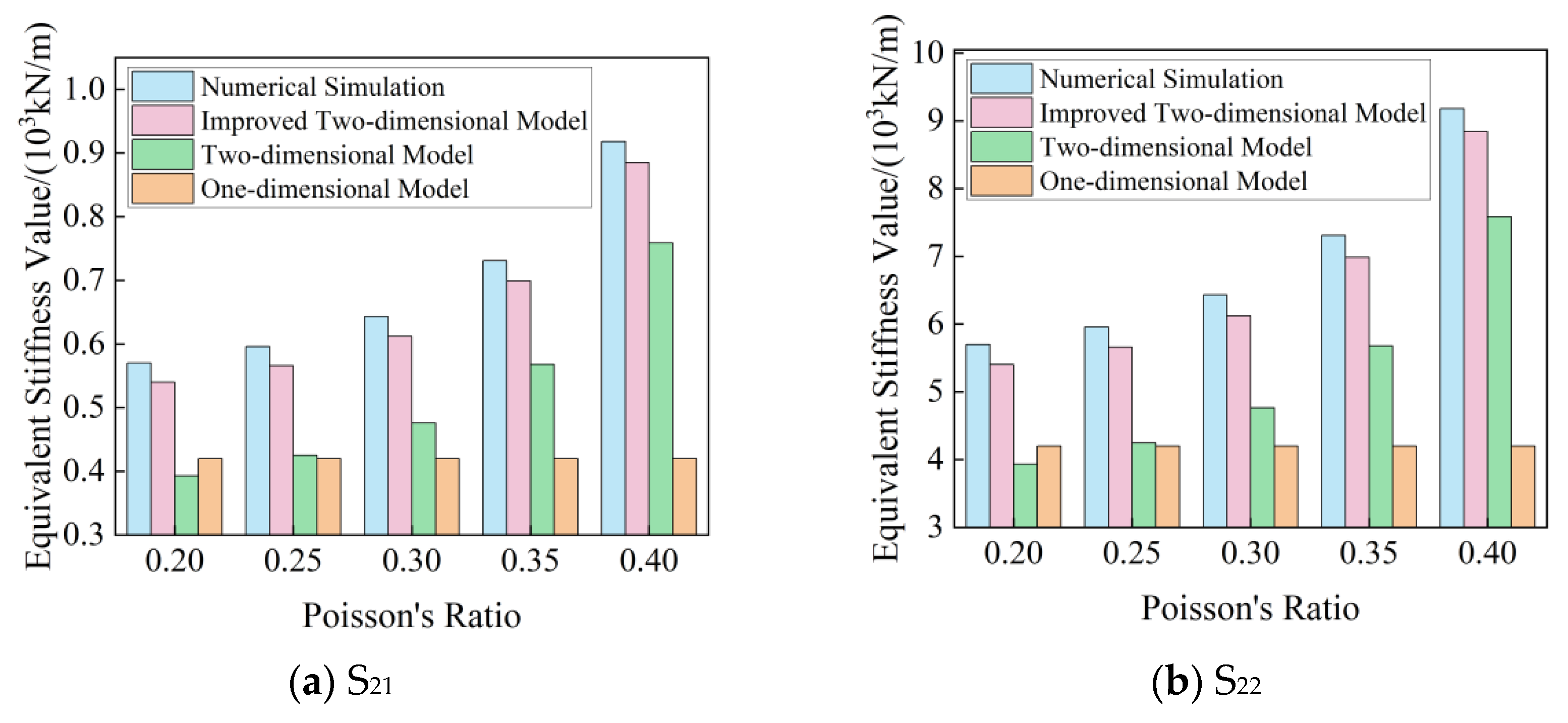
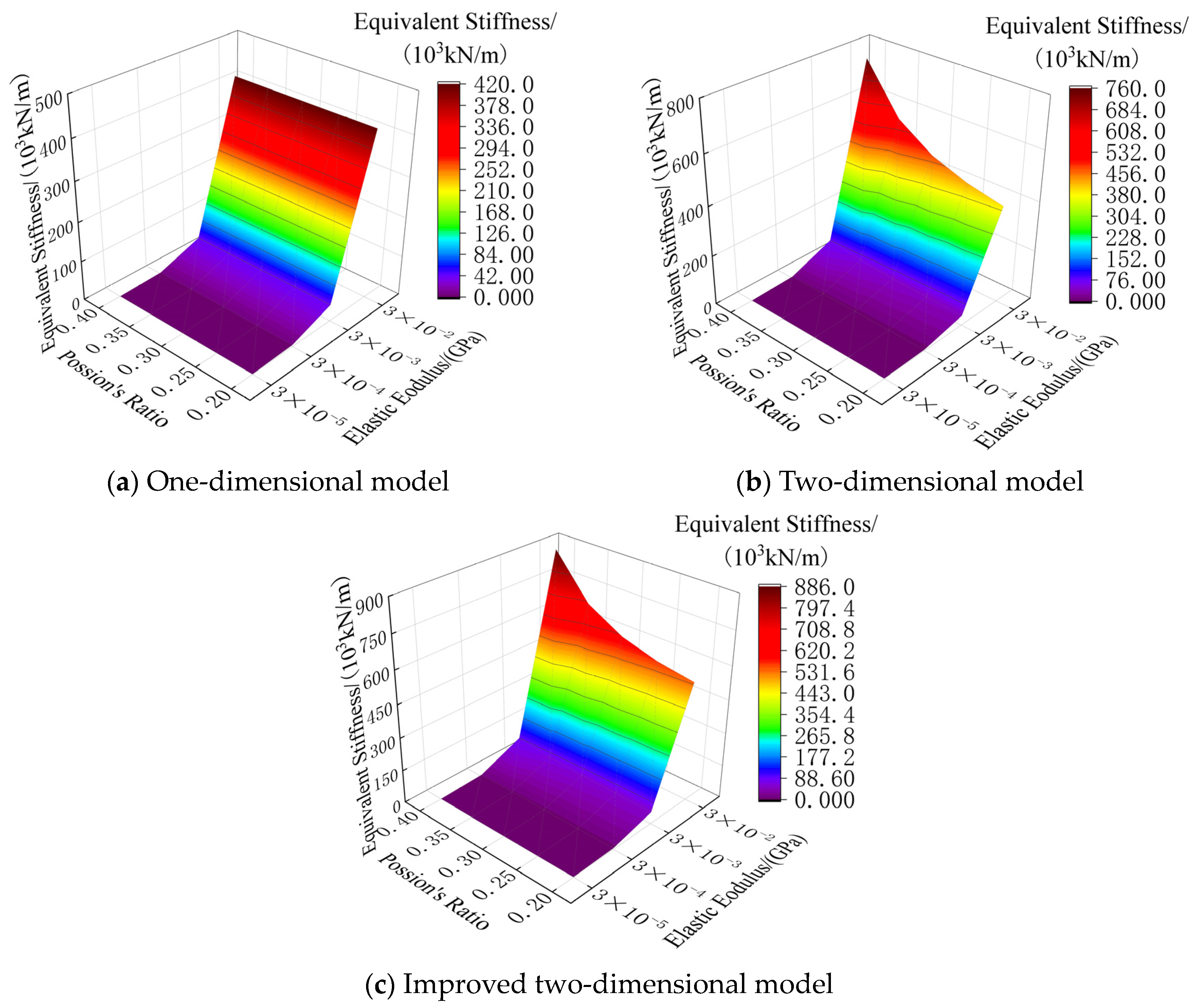
When the geometric parameters and elastic modulus of the coating remain unchanged, the prediction results of the one-dimensional vibration-theoretical model remain unchanged, and the error rate increases with the increase in Poisson’s ratio. The prediction results of the two-dimensional vibration theory model and the improved two-dimensional model increase with the increase in Poisson’s ratio, while the error rates decrease.

(3)

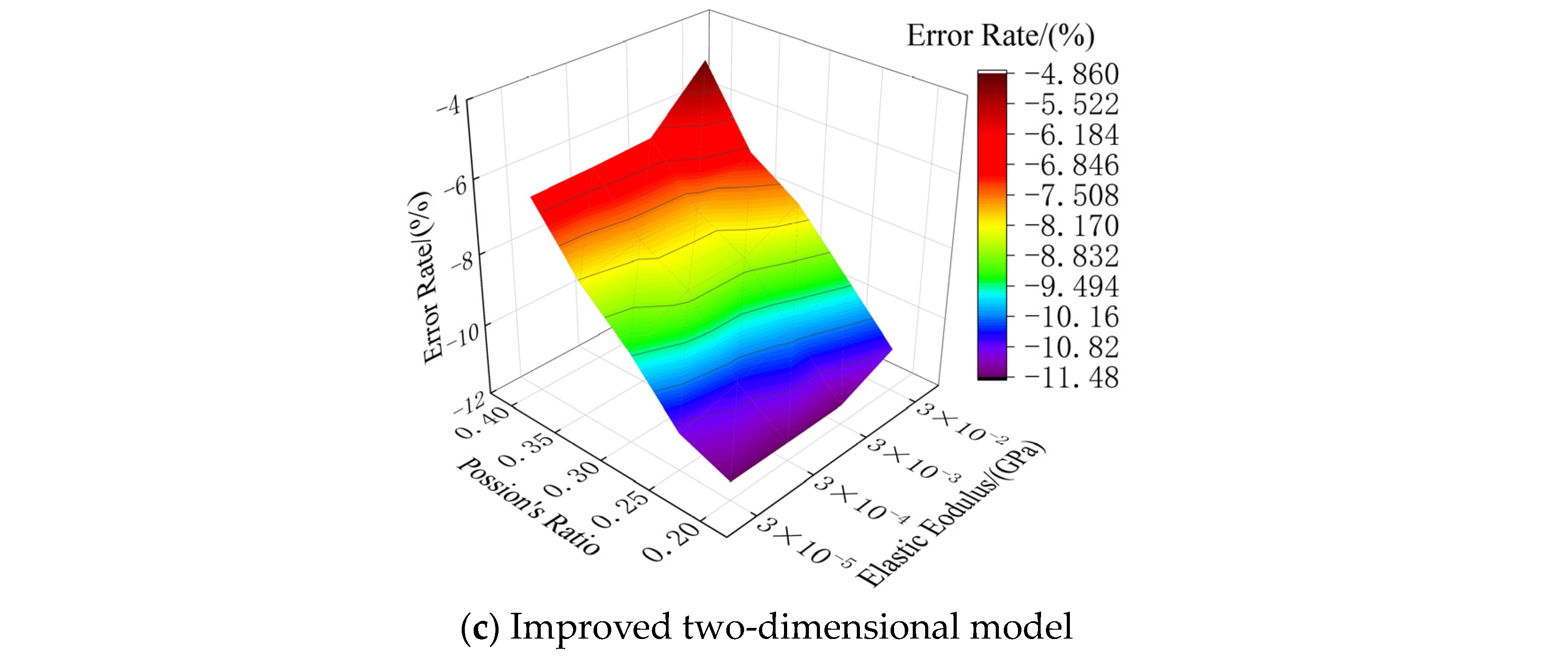
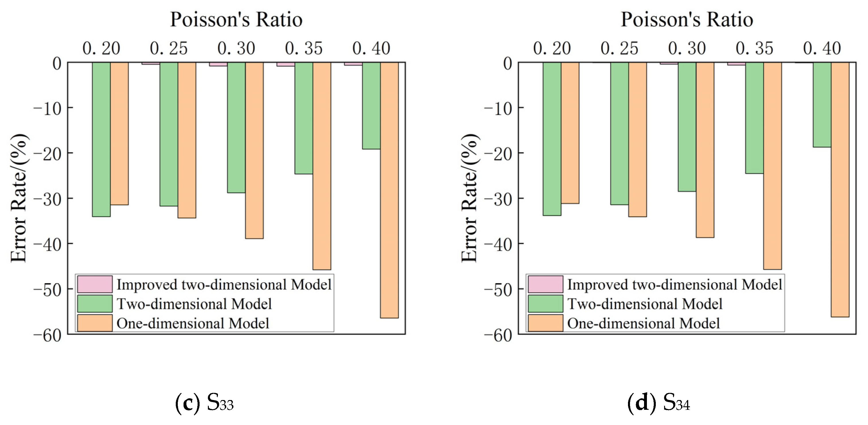
The one-dimensional theoretical vibration model cannot accurately predict the simulation results; in the research scope of this paper, the error rate is up to −56.49% (the negative sign means that the theoretical result is smaller than the simulation result). The two-dimensional theoretical vibration model is suitable for the case of a large elastic modulus, large Poisson’s ratio and thin coating thickness. In other cases, the error rate of the two-dimensional theoretical vibration model can reach up to −34.28%. The improved two-dimensional theoretical vibration model is applicable to all situations. The absolute value of the error rate of working condition 2 is generally within 5%, and it is generally within 1% for working condition 3. This shows that the improved two-dimensional theoretical vibration model proposed in this paper is more accurate, can better explain the vibration characteristics of the metamaterial concrete unit cell and is more suitable for the prediction of its equivalent stiffness value.

The proposed model provides simpler and more transparent descriptions of the underlying physical phenomena. It is derived from fundamental principles and equations, making it easy to understand the assumptions and limitations of the model. The proposed model can also be computationally more efficient compared to numerical methods like those used in COMSOL, since it requires less computational resources and time, which can be advantageous for quick analysis or exploration of a wide range of scenarios. In addition, the application of specific formulas to mathematical computation software can speed up the calculation of the equivalent stiffness values of a single metamaterial concrete unit cell under different parameter conditions compared to finite element software calculations. The theoretical formulation of equivalent stiffness can be established to solve the problem of a specific vibration isolation frequency in practical engineering, and in this way, we can determine the geometric and material parameters of metamaterial concrete according to the frequency range.

References

1. Wegener, M. Metamaterials Beyond Optics. Science 2013, 342, 939–940. [Google Scholar] [CrossRef] [PubMed]
2. Landy, N.; Smith, D.R. A full-parameter unidirectional metamaterial cloak for microwaves. Nat. Mater. 2013, 12, 25–28. [Google Scholar] [CrossRef] [PubMed]
3. Marunin, M.V.; Polikarpova, N.V. Polarization of Acoustic Waves in Two-Dimensional Phononic Crystals Based on Fused Silica. Materials 2022, 15, 8315. [Google Scholar] [CrossRef] [PubMed]
4. Li, B.; Tan, K.T.; Christensen, J. Tailoring the thermal conductivity in nanophononic metamaterials. Phys. Rev. B 2017, 95, 144305. [Google Scholar] [CrossRef]
5. Wang, Y.-Z.; Li, F.-M.; Wang, Y.-S. Influences of active control on elastic wave propagation in a weakly nonlinear phononic crystal with a monoatomic lattice chain. Int. J. Mech. Sci. 2016, 106, 357–362. [Google Scholar] [CrossRef]
6. Banerjee, B.; Nagy, P.B. An Introduction to Metamaterials and Waves in Composites. J. Acoust. Soc. Am. 2012, 131, 1665–1666. [Google Scholar] [CrossRef]
7. Al Ba’Ba’A, H.B.; Nouh, M. Mechanics of longitudinal and flexural locally resonant elastic metamaterials using a structural power flow approach. Int. J. Mech. Sci. 2017, 122, 341–354. [Google Scholar] [CrossRef]
8. Liu, X.N.; Hu, G.K.; Huang, G.L.; Sun, C.T. An elastic metamaterial with simultaneously negative mass density and bulk modulus. Appl. Phys. Lett. 2011, 98, 251907. [Google Scholar] [CrossRef]
9. Li, J.; Chan, C.T. Double-negative acoustic metamaterial. Phys. Rev. E 2004, 70, 055602. [Google Scholar] [CrossRef]
10. Xu, C.; Chen, W.; Hao, H.; Pham, T.M.; Li, Z.; Jin, H. Dynamic compressive properties of metaconcrete material. Constr. Build. Mater. 2022, 351, 128974. [Google Scholar] [CrossRef]
11. Ansari, M.; Tartaglione, F.; Koenke, C. Experimental Validation of Dynamic Response of Small-Scale Metaconcrete Beams at Resonance Vibration. Materials 2023, 16, 5029. [Google Scholar] [CrossRef] [PubMed]
12. Chen, Z.; Wang, G.; Lim, C. Artificially engineered metaconcrete with wide bandgap for seismic surface wave manipulation. Eng. Struct. 2023, 276, 115375. [Google Scholar] [CrossRef]
13. Xu, C.; Chen, W.; Hao, H.; Bi, K.; Pham, T.M. Experimental and numerical assessment of stress wave attenuation of metaconcrete rods subjected to impulsive loads. Int. J. Impact Eng. 2021, 159, 104052. [Google Scholar] [CrossRef]
14. Li, Q.Q.; He, Z.C.; Li, E.; Cheng, A.G. Design of a multi-resonator metamaterial for mitigating impact force. J. Appl. Phys. 2019, 125, 035104. [Google Scholar] [CrossRef]
15. Jin, H.; Chen, W.; Hao, H.; Hao, Y. Numerical study on impact resistance of metaconcrete. Sci. Sin. Phys. Mech. Astron. 2020, 50, 024609. [Google Scholar] [CrossRef]
16. Briccola, D.; Cuni, M.; De Juli, A.; Ortiz, M.; Pandolfi, A. Experimental validation of the attenuation properties in the sonic range of metaconcrete containing two types of resonant inclusions. Exp. Mech. 2020, 61, 515–532. [Google Scholar] [CrossRef]
17. Li, C.; Qing, H.; Ru, C.Q. On two initial-boundary-value problems for impact dynamics of metaconcrete rods. Eng. Math. 2023, 140, 5. [Google Scholar] [CrossRef]
18. Jin, H.; Hao, H.; Hao, Y.; Chen, W. Predicting the response of locally resonant concrete structure under blast load. Constr. Build. Mater. 2020, 252, 118920. [Google Scholar] [CrossRef]
19. Jin, H.; Hao, H.; Chen, W.; Xu, C. Effect of enhanced coating layer on the bandgap characteristics and response of metaconcrete. Mech. Adv. Mater. Struct. 2021, 30, 175–188. [Google Scholar] [CrossRef]
20. Gao, Y.; Wang, H. Comparative investigation of full bandgap behaviors of perforated auxetic metaconcretes with or without soft filler. Mater. Today Commun. 2024, 38, 108526. [Google Scholar] [CrossRef]
21. Xiao, P.; Miao, L.; Zheng, H.; Lei, L. Low frequency vibration reduction bandgap characteristics and engineering application of phononic-like crystal metaconcrete material. Constr. Build. Mater. 2024, 411, 134734. [Google Scholar] [CrossRef]
22. Xiong, J.; Ren, F.; Li, S.; Tian, S.; Li, Y.; Mo, J. A study on low-frequency vibration mitigation by using the metamaterial-tailored composite concrete-filled steel tube column. Eng. Struct. 2024, 305, 117673. [Google Scholar] [CrossRef]
23. Chen, B.; Zheng, Y.; Dai, S.; Qu, Y. Bandgap enhancement of a piezoelectric metamaterial beam shunted with circuits incorporating fractional and cubic nonlinearities. Mech. Syst. Signal Process. 2024, 212, 111262. [Google Scholar] [CrossRef]
24. Bae, M.H.; Oh, J.H. Nonlinear elastic metamaterial for tunable bandgap at quasi-static frequency. Mech. Syst. Signal Process. 2022, 170, 108832. [Google Scholar] [CrossRef]
25. Anigbogu, W.; Bardaweel, H. A Comparative Study and Analysis of Layered-Beam and Single-Beam Metamaterial Structures: Transmissibility Bandgap Development. Appl. Sci. 2022, 12, 7550. [Google Scholar] [CrossRef]
26. Jian, Y.; Hu, G.; Tang, L.; Xu, J.; Aw, K.C. A generic theoretical approach for estimating bandgap bounds of metamaterial beams. J. Appl. Phys. 2021, 130, 054501. [Google Scholar] [CrossRef]
27. Ma, Y.L.; Wang, X.M.; Mei, Y.L. Acoustic Metamaterials Composed of Pre-stressed Oscillator Unit Cells and the Effective Method of Adjusting and Expanding Bandgap. In Advances in Machinery, Materials Science and Engineering Application; License CC BY-NC 4.0; IOS Press: Amsterdam, The Netherlands, 2022. [Google Scholar] [CrossRef]
28. Cui, R.; Zhou, J.; Gong, D. Wave-resistance sleeper with locally resonant phononic crystals: Bandgap property and vibration reduction mechanism. AIP Adv. 2021, 11, 035043. [Google Scholar] [CrossRef]
29. Carvalho, A.L.L.; Gomes, C.B.F.; dos Santos, J.M.C.; de Miranda, E.J.P., Jr. Effect of Resonant Aggregate Parameters in Metaconcrete Thin Plates on Flexural Bandgaps: Numerical Simulations. Mater. Res. 2023, 26 (Suppl. 1), e20220547. [Google Scholar] [CrossRef]
30. Slesarenko, V. Bandgap structure in elastic metamaterials with curvy Bezier beams. Appl. Phys. Lett. 2023, 123, 081702. [Google Scholar] [CrossRef]
31. Chen, J.; Qu, Y.; Guo, Z.; Li, D.; Zhang, G. A one-dimensional model for mechanical coupling metamaterials using couple stress theory. Math. Mech. Solids 2023, 28, 2732–2755. [Google Scholar] [CrossRef]
32. Zhou, Y.; Ye, L.; Chen, Y. Developing three-dimensional mechanical metamaterials with tailorable bandgaps for impact mitigation. J. Phys. D Appl. Phys. 2024, 57, 195501. [Google Scholar] [CrossRef]
33. Zhang, E.; Lu, G.Y.; Yang, H.W.; Lin, S. Band gap characteristics of metamaterial concrete and its attenuation effect on shock wave. Explos. Shock. 2020, 502, 116088. [Google Scholar]
34. Han, J.; Lu, G.Y. A study of undamped free vibration characteristics on a metaconcrete unit cell. J. Vib. Shock 2021, 40, 173–178. [Google Scholar] [CrossRef]
35. Han, J.; Lu, G.Y.; Zhao, Y.T. A study of damped free vibration characteristics on a metaconcrete unit. J. Vib. Shock 2022, 41, 31. [Google Scholar] [CrossRef]
36. Han, J.; Lu, G. Study on damping forced vibration characteristics of metamaconcrete unit cell and optimizing aggregate selection. Constr. Build. Mater. 2024, 421, 135598. [Google Scholar] [CrossRef]
37. Bo, Z.; Li, Z. New Analytical Model for Composite Materials Containing Local Resonance Units. J. Eng. Mech. 2011, 137, 1–7. [Google Scholar] [CrossRef]
38. Vo, N.H.; Pham, T.M.; Bi, K.; Chen, W.; Hao, H. Stress Wave Mitigation Properties of Dual-meta Panels against Blast Loads. Int. J. Impact Eng. 2021, 154, 103877. [Google Scholar] [CrossRef]
39. Vo, N.H.; Pham, T.M.; Bi, K.; Hao, H. Model for analytical investigation on meta-lattice truss for low-frequency spatial wave manipulation. Wave Motion 2021, 103, 102735. [Google Scholar] [CrossRef]
40. Yu, J.; Jung, J.; Wang, S. Derivation and Validation of Bandgap Equation Using Serpentine Resonator. Appl. Sci. 2022, 12, 3934. [Google Scholar] [CrossRef]
41. Wen, X.S.; Wen, J.H.; Yu, D.L. Phononic Crystal; National Defense Industry Press: Arlington, VA, USA, 2009. [Google Scholar]
42. Oyelade, A.O.; Abiodun, Y.O.; Sadiq, M.O. Dynamic behaviour of concrete containing aggregate resonant frequency. J. Comput. Appl. Mech. 2018, 49, 380–385. [Google Scholar] [CrossRef]
43. Gao, Y.J.; Fan, H.L.; Zhang, B.; Jin, F.N. Research on the clipping effect of metamaterial wave-absorbing concrete slabs under the action of two-dimensional plane waves. J. Vib. Shock 2018, 37, 39–44. [Google Scholar] [CrossRef]
Figure 1. Metamaterial concrete unit cell.
Buildings 14 01035 g001
Figure 2. Simplified model of metamaterial concrete unit cell.
Buildings 14 01035 g002
Figure 3. One-dimensional metamaterial concrete lattice system.
Buildings 14 01035 g003
Figure 4. Simplified element model.
Buildings 14 01035 g004
Figure 5. Element calculation model.
Buildings 14 01035 g005
Figure 6. Metamaterial concrete model.
Buildings 14 01035 g006
Figure 7. Schematic diagram of the selection of equivalent stiffness for the improved two-dimensional model.
Buildings 14 01035 g007
Figure 8. Equivalent stiffness of the improved two-dimensional theoretical vibration model and numerical simulation results in working condition 1.
Buildings 14 01035 g008
Figure 9. Error ratio of the improved two-dimensional theoretical vibration model and numerical simulation results in working condition 1.
Buildings 14 01035 g009
Figure 10. Equivalent stiffness in working condition 1.
Buildings 14 01035 g010
Figure 11. Error rate in working condition 1.
Buildings 14 01035 g011aBuildings 14 01035 g011b
Figure 12. Equivalent stiffness of the improved two-dimensional theoretical vibration model and numerical simulation results in working condition 2.
Buildings 14 01035 g012aBuildings 14 01035 g012b
Figure 13. Error ratio of the improved two-dimensional theoretical vibration model and numerical simulation results in working condition 2.
Buildings 14 01035 g013
Figure 14. Equivalent stiffness in working condition 2.
Buildings 14 01035 g014
Figure 15. Error rate in working condition 2.
Buildings 14 01035 g015
Figure 16. Equivalent stiffness of the improved two-dimensional theoretical vibration model and numerical simulation results in working condition 3.
Buildings 14 01035 g016
Figure 17. Error ratio of the improved two-dimensional theoretical vibration model and numerical simulation results in working condition 3.
Buildings 14 01035 g017aBuildings 14 01035 g017b
Figure 18. Equivalent stiffness in working condition 3.
Buildings 14 01035 g018aBuildings 14 01035 g018b
Figure 19. Error rate in working condition 3.
Buildings 14 01035 g019