Technical Note

Precision of Measurements of Delayed Slip in Structural High-Strength Assemblies by Contact and Optical Methods

1
ETSI Minas y Energía, Universidad Politécnica de Madrid, C/ Alenza 4, 28003 Madrid, Spain
2
School of Civil Engineering and Architecture, Xinjiang University, Urumqi 830047, China
3
ETSI Caminos, C. y P., Universidad de Castilla-La Mancha, Av. Camilo José Cela s/n, 13071 Ciudad Real, Spain
4
E. I. Minera e Industrial de Almadén, Universidad de Castilla-La Mancha, Pza. Manuel Meca 1, 13400 Almadén, Spain
*
Author to whom correspondence should be addressed.
Buildings 2024, 14(4), 1046; https://doi.org/10.3390/buildings14041046
Submission received: 29 December 2023 / Revised: 26 March 2024 / Accepted: 4 April 2024 / Published: 9 April 2024
(This article belongs to the Special Issue Performance Analysis of Steel Structure in Construction)

Abstract

:
Structural bolted connections of steel plates must fulfill the requirements specified by the standard EN 1090-2:2018 in the European Union. For the slip-resistant joints, the standard establishes the experimental procedure to obtain the delayed slip under a constant loading, which should not exceed 2 μm from the first five minutes to three hours. However, the usual extensometers available in laboratories, like LVDTs, lack the necessary precision to obtain a reliable measurement of such a small displacement because, even if their resolution is 1 μm, the scatter of repeated measurements of the same distance is normally higher. In contrast, the resolution and precision in optical methods like Digital Image Correlation (DIC) can be easily set under 1 μm depending on the number of pixels covering the studied area and the performed subpixel interpolation. This work introduces the use of DIC for delayed slip tests. In comparison with an LVDT, it is verified that this technique is a valid alternative to measure displacements at that scale with a simpler experimental setup.

1. Introduction

Steel structures are made of a series of structural members that are produced and shaped in a factory or workshop and that are later assembled at the construction site. Two main assembly methods are used [1,2]. On the one hand, two steel members can be joined by a welded connection where their base material is fused with a molten filler metal so that a continuous solid material is formed between both when it cools. On the other hand, they can be joined by a bolted connection. In this case, a certain flat portion of their length can be overlapped, if the shape of the members allows it, or auxiliary plates can be used to create a bridge between them. Then, the different layers are pressed together by some tightened bolts that pass through them.
Focusing on bolted joints, in cases when it is necessary to avoid the relative displacement between both members, their contact must be resistant to slip movements. With this purpose, the contact surfaces have to be prepared to achieve the required slip factor. This is achieved, for example, by blasting the metal surface with grit. The capacity of bolted assemblies against slip is controlled in European countries by the requirements of the standard EN 1090-2:2018 [2,3,4]. In particular, Annex G of this document establishes the procedure for the experimental determination of the friction coefficient provided by the applied surface treatment depending on the obtained slip force and the preloading of the bolts. Moreover, the standard sets what is the admissible evolution of the possible slip under a given constant loading along the service life of the structure. In order to fulfill this requirement, the delayed slip after three hours in a test at a constant loading equal to 90% of the mean slip force previously determined must not exceed 2 μm.
However, this slip tolerance poses the problem of the measuring accuracy that is necessary to check this requirement. In the present work, it is emphasized that common measuring instruments for displacements that are used in testing laboratories lack the needed precision to provide a reliable measurement at that scale. These contact extensometers, mainly Linear Variable Differential Transducers (LVDT) and clip-on extensometers, generally have measuring resolutions of 1 μm, which is just 50% of the total allowed relative displacement during the test. In any case, the real problem lies in the precision of the instrument, which is usually worse than that resolution, meaning that repeated measurements of the same distance will vary among them by more than 1 μm. This is what marks the lower limit of the range of applicability of these tools. Therefore, accurately measuring a slip of 2 μm will be beyond the possibilities of most devices, even if they provide measurements at the micrometer level. More specialized extensometers [5] are capable of measuring displacements with the required precision, but they are less affordable and their measuring range is rather limited, which is inconvenient for the particular application treated here.
In contrast to the measuring methods based on contact extensometers, optical methods offer an alternative with a wider range of possibilities. For example, small displacements of moving objects can be measured from videos of fast cameras by applying the phase-based motion magnification technique [6,7]. This consists in decomposing the original video signal into sinusoidal waves, which are magnified and reassembled later. The modified video is read by software with algorithms to follow the movement of key points on the studied object. Another example is the use of 2D or 3D laser Doppler vibrometers. Applied mainly for vibrations, they are based on the Doppler effect by detecting the change in wave frequency of the oscillating movement from the object to the laser measuring device, which allows displacements to be computed [8].
Among these optical techniques, one of the most popular ones that has experienced a large development since it first appeared [9,10,11] is the Digital Image Correlation (DIC) method [12]. This is a full-field method, as it can compute the displacement of a series of rectangular or square regions that are distributed all over a given portion of the surface of the studied material. This is achieved by tracking their centers through a sequence of pictures taken during the deformation process of the specimen. The complete displacement field on the surface, from which the strain field can be derived, is obtained by the proper interpolation between those points.
The DIC method can be applied independently of the scale of the dimensions of the studied surface because the basic length unit in the method is the pixel width of the digital images that are used. Therefore, the displacements on the real surface are obtained by scaling that width to the corresponding length. This means what counts is the area of the material surface covered by the images, which can range from photographs of real-scale structural elements [13] to micrographs [14]. The application field where DIC is more extensively used is in experimental tests for the mechanical characterization of materials, with a scale in the range of millimeters to hundreds of millimeters [15]. By means of the interpolation methods, displacements on the surface can be provided even at levels as refined as lengths corresponding to 0.0002 pixels [16], although the precision of those measurements keeps in practice a certain minimum proportion in relation to the size of the analyzed surface due to a series of unavoidable error sources of the experimental setup [17].
With this background in sight, the present work tries to warn about the significance of the measuring precision that is required for the delayed slip tests prescribed by the standard [2]. One of the characteristics of the DIC technique is that its variable resolution can be adequately set below 1 μm. Therefore, the objective of this study is to analyze if this method is valid to assess, with the necessary accuracy, the requirement of the standard on the maximum admissible delayed slip. In previous research by other authors [18,19,20], DIC has already been applied to measure the relative slip between two steel plates in a bolted assembly. The novelty introduced here is to use it for measurements within that smaller displacement range at the micrometer scale as a plausible alternative to traditional contact devices for this standardized test. With this aim, the scope of the study includes the comparison of results collected by means of an LVDT and DIC used simultaneously.
A brief description of both measuring techniques is offered in the next section. The specimen and the performed test are described later and, finally, the results are discussed and the conclusions of the study are presented.

2. Measuring Methods

2.1. LVDT

LVDTs are transducers that relate the movement of a ferromagnetic bar inside a series of windings and the induced electrical current that this generates [5]. The casing of the LVDT is fixed to a certain point, and the extreme of the bar is pressed to another one, so the LVDT measures the relative displacement between both points along the direction of the central axis of the instrument. Transverse movements must be avoided as the lateral friction of the bar inside the LVDT affects the measurement.
The precision of this type of device is usually provided as a percentage of the full range of measurements that they cover. For clarity, the term precision is defined as ‘the closeness of agreement between independent test results obtained under stipulated conditions’ [21,22]. In other words, the precision is related to the deviation of several measurements taken with the same device of a given distance. Apart from how close these measurements are among them, the accuracy of the measuring instrument consists in how close said measurements are to the real value of that distance. The accuracy can be controlled by the correct calibration of the instrument, but the precision depends on its design and determines the intrinsic measuring error of the device.
Table 1 presents the displacement error that can be expected in LVDTs for different combinations of typical measuring ranges and precision levels based on information from different providers, (for example, HBM (Darmstadt, Germany), models WA-T, WA-L and WI; Burster (Gernsbach, Germany), Models 8740 and 8741; Applied Measurements (Aldermaston, Berkshire, UK), AML/E series; TE Connectivity (Berwyn, PA, USA), GCA and HC-485 Series; Meggitt (Sensorex) (Archamps, France), models SX20MD and SX20MExR; etc.). The case that attains the lowest error is the one with the shortest range and the best precision. However, its error can be as high as 1 μm, which, even in this case, raises the issue of the suitability of its use to measure a maximum admissible slip displacement of 2 μm in the practical application treated in this study. Other cases in Table 1 could be directly rejected for this application.

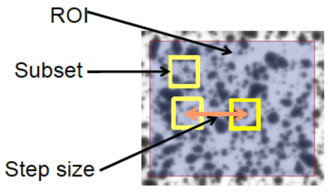
2.2. Digital Image Correlation

The Digital Image Correlation (DIC) method consists in establishing the correspondence of centers of facets located on a surface between a reference and the subsequent state. The images have to cover the area of the surface that must be analyzed, known as the Region of Interest (ROI). The surface must have a color gradient in both directions of its plane that facilitates the identification of those points on each image. Regarding surfaces with low contrast, artificial patterns of dots can be added. In these cases, it is usual to paint the surface white, first, adding black dots afterward.
The correspondence between points on different images can be established by either a global or a local approach [14]. In the former, the complete pattern of points on the ROI is analyzed in order to perform the match between them. In the latter case, however, the studied area is subdivided into smaller regions known as subsets with a certain size in pixels. This is the most common approach, as it was the first type that was used [9]. A series of subsets distributes over the ROI. The distance between the center points of neighbor subsets is the step size (Figure 1) [12,23]. The patterns of points or color gradients are locally analyzed within those subsets so that they can be detected between different images. Then, it is possible to determine the transformations experienced by the subset, like translation, rotation, and linear and angular deformations. After having computed the transformations of each subset, interpolation algorithms are applied to determine the complete displacement field on the surface. In this step, computations performed in terms of pixels are translated to length units by establishing the appropriate scale between the image and the real surface.
By means of those algorithms, it is possible to reach precision measurements at subpixel scales [24]. Most of the effort put into the development of the method consists in the improvement of the interpolation algorithms [16,25,26,27]. For this, synthetic images prepared so that the real displacement field is already known are usually employed to compare the solution given by the DIC method. The achieved precision can be 0.01 pixels [24,28,29] and even better [16]. However, in real experimental images, various error sources can affect the quality of the correlation method [17,30,31]. Some other articles focus on improving the efficiency of the algorithms to reduce the computation time [32,33]. The development of the DIC method is still open [34,35].

3. Experimental Test
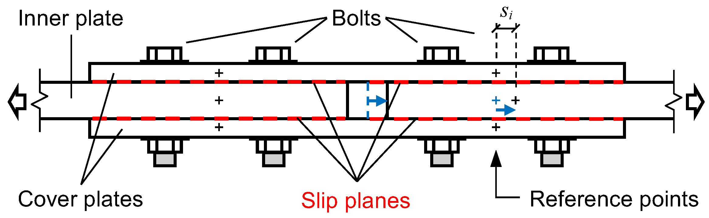
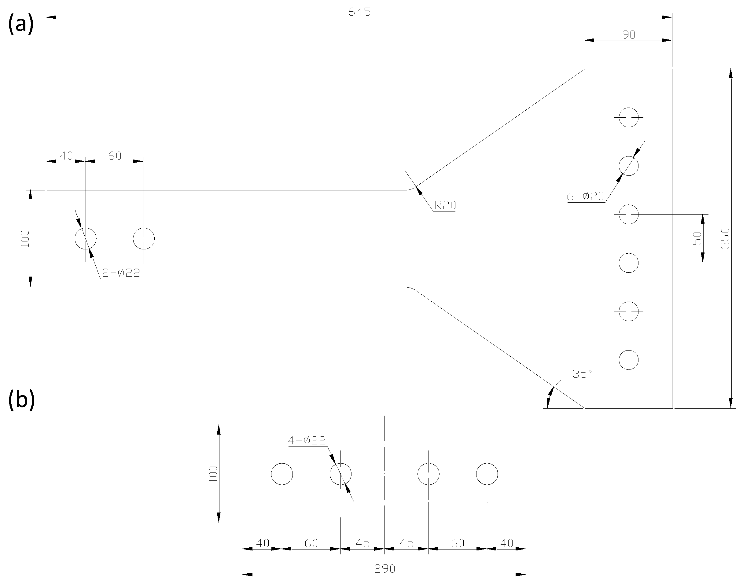
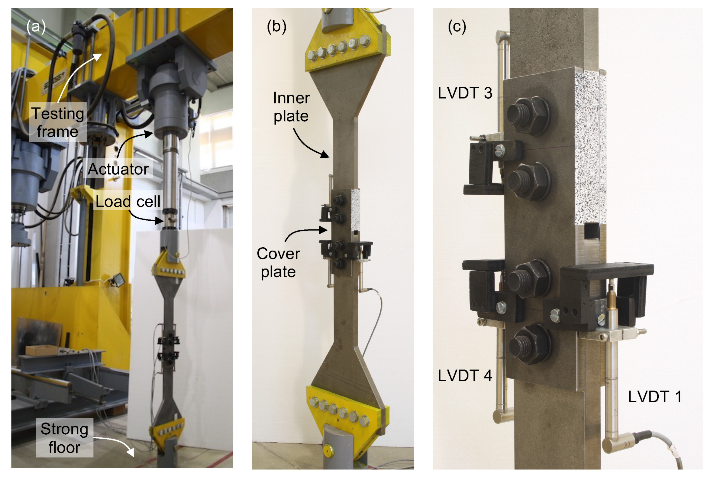
3.1. Specimen

A slip test was performed following the indications stated in Annex G of the standard EN 1090-2:2018 [2]. The first step was to produce the specimen for the test. This specimen is composed of four steel plates of two different types. These are two inner plates that are connected by two cover plates, one on each side of the inner plates. The material of the plates was a low-carbon steel grade S355J2. The surface of the plates was treated by blasting with a shot of copper slag in order to create enough roughness to reach the friction coefficient needed for the destination structure. This type of connection and material can be found, for instance, in pin-jointed trusses of roofs of industrial and sports installations.
All plates in the region of the assembly have the dimensions specified in the standard. The thickness of the inner plates is 20 mm, and the one of the cover plates is 10 mm. The width of both types of plates is 100 mm. The length of the cover plates is 290 mm, while the inner plates have to be at least longer than half of that length so that they extend beyond the cover plates after assembling the specimen. The outer extreme of the inner plates was shaped with a larger width, 300 mm, in order to reduce the stress concentration at the anchoring points and to transmit a uniform distributed stress to the area of contact between the inner and cover plates. For this same purpose, the total length of the inner plates was set as 645 mm. This design also favors stability against the rotation around the axis perpendicular to the plate. A schematic diagram with the shape and dimensions of the different plates of the specimen is shown in Figure 2.
Each inner plate is fixed to both cover plates by means of two high-strength bolts M20 × 70 10.9 HV, with a diameter of 20 mm. The holes for the bolts have an extra diameter of 2 mm with respect to the bolts. In this manner, the plates can be assembled so that there is enough margin for the slip displacement during the test.
The bolts were tightened so as to reach a load ( F p , C ) in their shaft equivalent to 70% of their strength ( f u b ), which for bolts M20 and quality 10.9 corresponded to F p , C = 0.7 f u b A s = 172 kN. For this, the torque method was applied by means of a wrench with a capacity of 1500 Nm. The four bolts were tightened in different steps of increasing torque following the same sequence in each step: the inner bolts in the first place and the outer ones next.

3.2. Slip Measurements

3.2.1. LVDT

Following the standard, displacements have to be measured at the four slip planes, which are both contact surfaces of both inner plates, and at both sides of the specimen, that is, the thickness side of the plates. Therefore, a total of eight independent measurements could be obtained. In any case, these eight measurements have to be grouped depending on the undergone slip process to provide two mean values per specimen. Each slip displacement between an inner plate and a cover plate is measured between two points centered on the thickness of their corresponding plate, which are initially leveled in the direction of the load at the mid position between the two holes for the bolts in the inner plates. Figure 3 sketches the assembly of the plates and the position of the reference points for slip measurements.
In order to measure the slip by means of LVDTs, there are different conditions to meet. In the first place, eight LVDTs would be necessary following the instructions of the standard. They would need to be fixed at the reference points on the sides of the cover plates, and they would measure against a stop object fixed at the reference point on the corresponding inner plate.
In the second place, the precision should be enough to measure a displacement of 2 μm for the delayed slip test. For this, if the LVDTs were to be chosen from Table 1, only the LVDT with a total measuring range of 1 mm and a precision of 0.10% would be an adequate candidate.
In the third place, however, it would be appropriate that the range of the LVDTs could cover the length of the total possible slip displacement of the plates, which is the 2 mm clearance between the bolts and the holes. This conflicts with the previous condition. There is no obligation to carry this out, but it is convenient for two reasons. On the one hand, the delayed slip test continues after the loading phase under a sustained force until the complete slip of the plates to obtain another value of the slip factor. On the other hand, an early failure of the assembly can take place either before or during that phase. If the range of the LVDTs is shorter than that maximum slip, it is necessary to place the LVDTs so that they start the test with their tip compressed and the direction of the slip must decompress the LVDTs until they lose contact with the reference point at the end of their measuring range, while the slip continues until the complete slip of 2 mm. In the opposite case, if the displacement direction of the slip compresses the LVDTs, the maximum slip could not be larger than 1 mm so as not to damage them. Due to the configuration of this type of test, the inner plates are pulled outwards from the assembly. This means that the LVDTs should be placed over the central part of the specimen pointing towards its ends so that they decompress during the slip displacement.
The size of small LVDTs is around 45–60 mm plus the length of the probe at one extreme and, possibly, the cable at the other extreme. Their diameter is around 20 mm. On each side of the bolted assembly, four of these LVDTs would have to be stably fixed to the cover plates at the reference points, which form a rectangle of 150 mm × 30 mm. Furthermore, at the middle point of the 30 mm sides, the stop objects that mark the reference point on the inner plates would also have to be fixed, between two LVDTs each. Finally, the four LVDTs would have to be aligned with the slip direction as well as possible.
These observations make clear that it is very difficult to arrange all these elements in that space and obtain precise measurements. For these reasons, the procedure to measure slip displacements by LVDTs was adapted here, as shown in Figure 4. On the one hand, LVDTs with a range larger than 2 mm were chosen. In particular, LVDTs HBM with a range of 10 mm were used. On the other hand, instead of independently measuring the relative slip in all contact surfaces, an averaged measurement of the slip of each inner plate with respect to both cover plates is obtained. With this aim, an LVDT is fixed to the inner plate by a metallic support. This support is held by a small screw at the center point of the plate thickness. The probe tip is in contact with a flat piece that is anchored at both sides to the cover plates at points leveled with the fixing point of the LVDT. In this case, the LVDTs have to be placed pointing to the central part of the assembly but, as they are fixed to the inner plate instead, the slip displacement tends to decompress the probe.
With this setup, four LVDTs are needed to measure the mean slip at both sides of the inner plates (Figure 4a). In the case of the delayed slip test, the position of one of them was prepared to apply the DIC method (Figure 4b,c), so only three LVDTs were used in this case.
As this type of LVDT is expected to lack the necessary precision, a verification of their measurement was performed with a calibrated extensometer, a Sylvac Dial Gage S229 with a repeatability of 2 μm. The following procedure consisted in comparing repeated measurements of each LVDT with those given by the reference extensometer at different points along their complete 10 mm range, with intervals of 0.5 mm (Figure 5). In the figure, the vertical axis represents the difference in the displacement measurement Δ s given by the instrument between two consecutive steps. The measurements were taken in both directions, compressing and decompressing the LVDT. The measurement error in a displacement of 0.5 mm is obtained as e = Δ s 0.5 . This type of error is related to the nonlinearity of the instrument.
As shown in Figure 5, the mean absolute error for this step size was 4 μm in the four LVDTs. Figure 5 allows us to check, as well, how the error varies along the measuring range. In certain sections, the error is minimum, below 1 μm, but in other sections, the error can reach 8–10 μm. In one case, the maximum error reached 23 μm, although this measurement could be considered an outlier as it is not in consonance with the tendency of the error in that section of the range.
Regarding precision, following its definition, it consists in the difference between the measurements of a given distance. The precision values obtained are 4 μm, 4 μm, 3 μm, and 2 μm, respectively, from LVDT 1 to LVDT 4, discarding the outlier value in LVDT 3. Expressed as a percentage of the range, the worst precision is 0.04%, which is very good in comparison with common reference values from manufacturers in Table 1. In any case, this is a simple estimation, as only a couple of measurements were taken at each one of the selected points along their range. Increasing the number of repeated measurements will initially increase the scatter of the obtained values and, thus, the precision error that the instrument presents in reality.

3.2.2. DIC

In order to employ the DIC method in the delayed slip test, a side of the specimen in the overlapping area of the cover plates with one of the inner plates was prepared as the ROI by creating a speckle pattern of black dots on the surface painted in white (Figure 4c). The random pattern was created by spraying the black ink. Two lamps lit the surface during the test.
Digital images were taken by means of a Canon EOS 1000D digital SLR camera (Canon, Tokyo, Japan) with an APS-C sensor with a resolution of 3888 × 2592 pixels (10 megapixels). Different recommendations for 2D-DIC systems were followed to minimize error sources in the application of the DIC method [23]. The camera was equipped with a Canon EF-S lens with a fixed focal length of 60 mm, which allowed reducing angular distortions. The camera was mounted on a tripod with its optical axis perpendicularly directed towards the specimen surface. It was placed at a distance of 1.5 m in order to cover the full 135 mm × 40 mm domain so that the whole speckle pattern filled the image. Pictures were taken with the same exposure time at uniform intervals of 2 min during the test and with the autofocusing function switched off.
The DIC analysis was performed with the commercial software VIC 2D, appropriately setting the different analysis parameters [23]. As the initial step, input images were prepared by automatically converting them into grayscale ones and by removing some high-frequency information through a low-pass filter. The subset size was established as 41 pixels, while the step size was 10 pixels. The adopted matching or correlation criterion was the normalized sum of square differences. A Gaussian subset weight function was used so as to give a higher influence on the correlation to the pixels closer to the central point of the subset. The applied computational method was the Forward Additive Newton–Raphson algorithm.
Due to the combination of the distance of the camera to the specimen and the focal length that was used, the complete thickness of the three layers of plates in the ROI, 40 mm, corresponded to 1014 pixels in the digital image. As a result, the pixel width was equivalent to 39 μm. The final resolution was set to 0.39 μm by considering 100-pixel subdivisions by means of an optimized 8-tap interpolation function. Taking into account the considerations introduced in the description of the method, the precision of the measurements made by means of the DIC analysis, or displacement accuracy, is equivalent in magnitude to the resolution, so it can be taken as 0.4 μm, by rounding that value. Therefore, the precision of the DIC method is around 5 to 10 times better than the LVDTs used in the test.

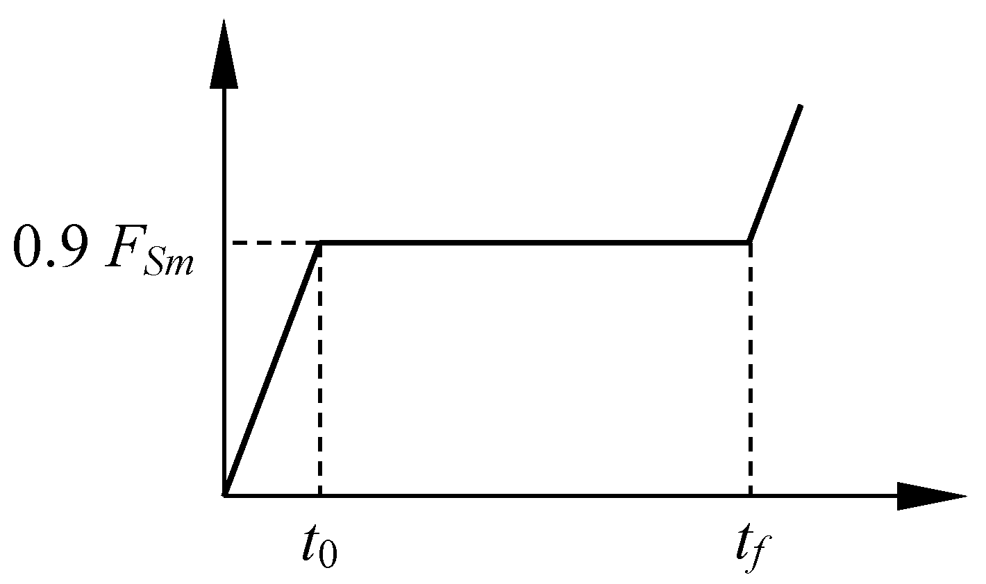
3.3. Experimental Procedure

The testing machine consisted of a servo-hydraulic Servosis actuator mounted on a steel testing frame, with a load cell with a maximum capacity of ±1000 kN. The specimen was placed vertically, anchoring the bottom part to the strong floor of the laboratory and the upper part to the actuator. Figure 4a shows the testing equipment with a specimen.
Two types of tests are necessary to characterize the behavior of bolted joints against slip [2]. Firstly, four specimens must be tested under a monotonically increasing force until completing the possible slip displacement in every contact surface of the assembly. From the force–displacement curve provided by each LVDT, the slip force is obtained as the highest force value within the first interval of 0.15 mm of slip displacement.
Secondly, the delayed slip experienced by the joint under a sustained force is assessed by a creep test. In this test, the force is increased until 90% of the mean slip force obtained in the previous tests, and then it is maintained at that value for three hours. After that time, the loading continues increasing in order to obtain the slip force with the criterion expressed before. Only one specimen is initially needed for this test. If the slip that takes place during the interval from the first five minutes under the sustained force until the three hours keeps under a tolerance displacement of Δ s tol = 2 μm, the requirement of the standard for delayed slips is fulfilled, and no more tests are necessary. In the case that the measured slip in that time interval is higher, then at least three additional extended creep tests are necessary. In this case, the phase of constant load has to be maintained during the time necessary to check that the extrapolated slip during the design life of the structure, with time in logarithmic scale, does not exceed 0.3 mm.
The final result of this series of tests is the mean slip factor of the treated steel surface, obtained as the coefficient between the slip forces and the transverse load applied by the four high-strength bolts. The work presented in this article focuses on the delayed slip or creep test to compare the adequacy of both measuring methods to verify if the displacement is under Δ s tol . Therefore, the slip force could be characterized by one test, and only the results corresponding to the delayed slip are discussed.
This test was performed by controlling the force signal of the testing machine (Figure 6). The loading ramp until the phase of constant value of force was applied at a velocity of 0.5 kN/s.

4. Results

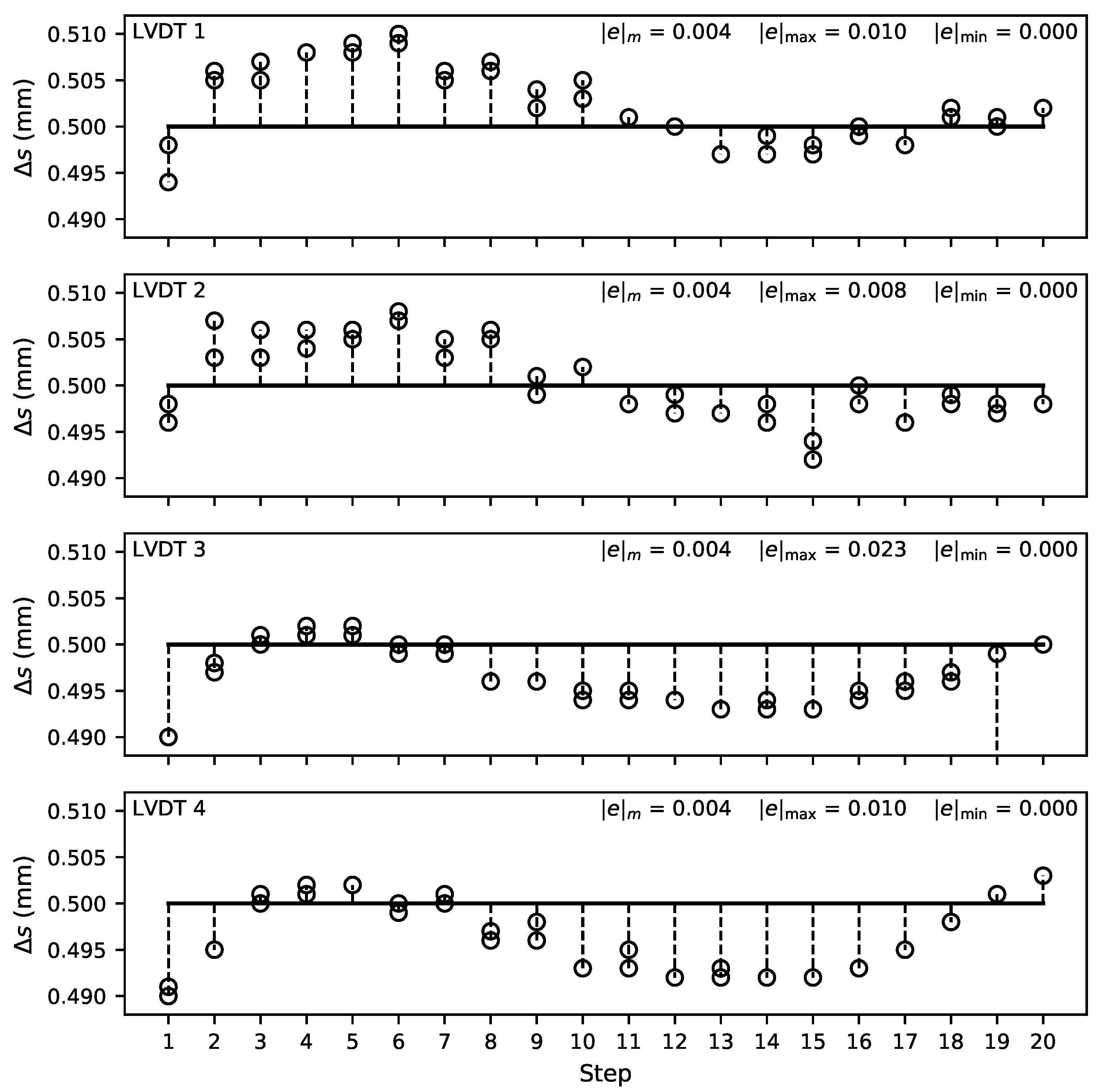
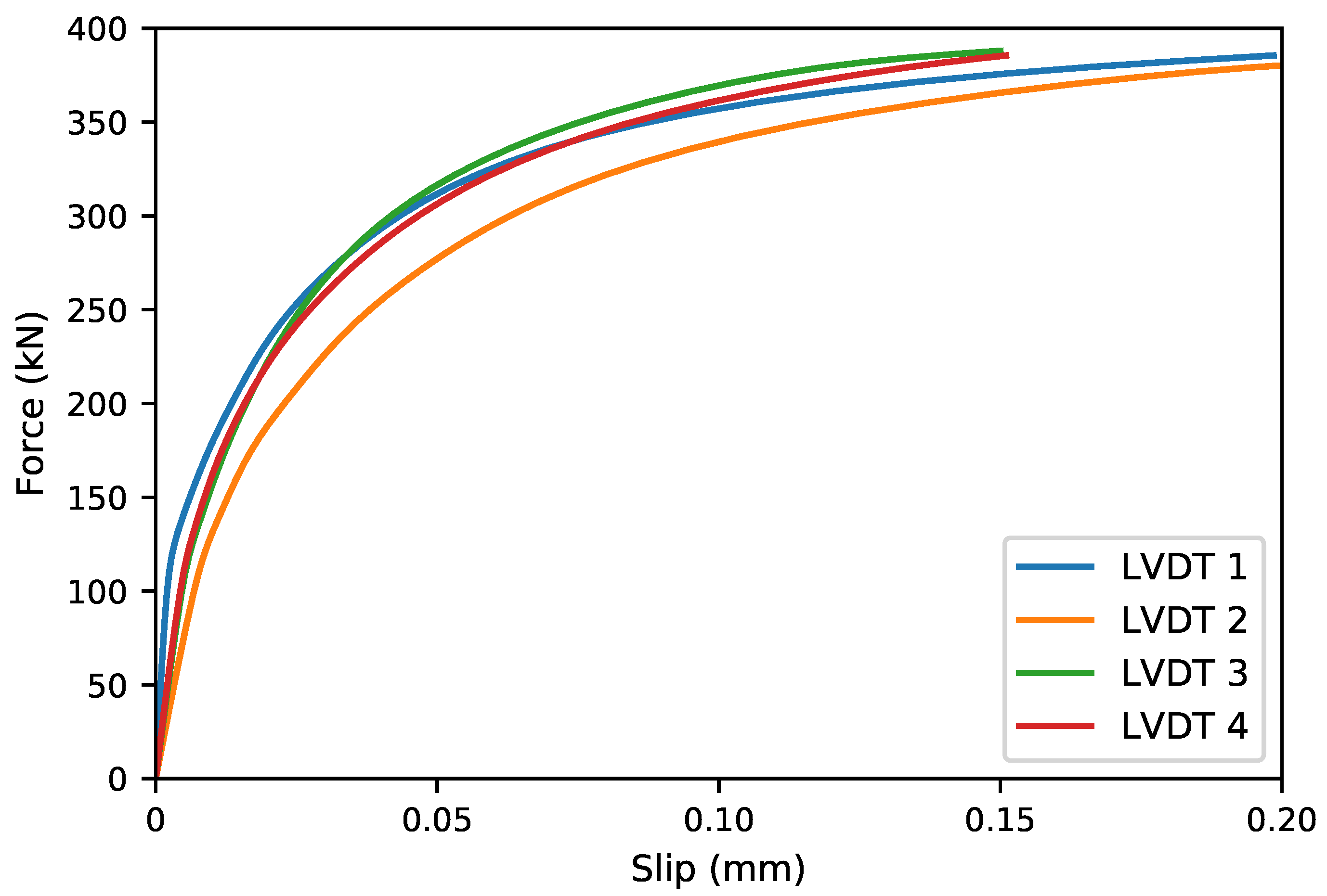
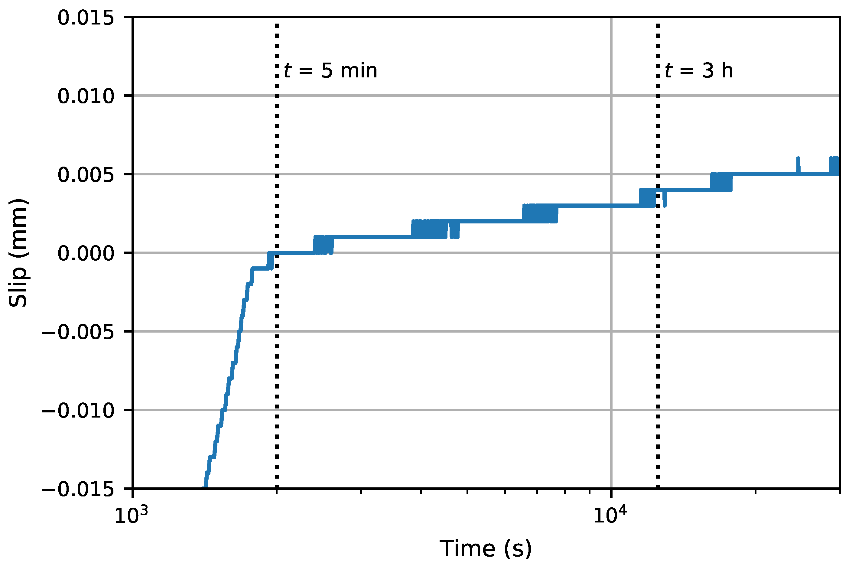
4.1. LVDT Measurement

The slip resistance was determined from the curves of Figure 7. The corresponding slip force values were 378 kN, 367 kN, 387 kN, and 385 kN, so the obtained mean slip force was F S m = 379 kN. As a result, the constant force for the delayed slip test resulted in 341 kN.
With respect to the displacements measured by the LVDTs, the result of interest from this test is the slip measurement provided by the LVDT placed on the same inner plate onto which the optical method is applied. It is considered that they are directly comparable because the rotation between the inner and cover plates is not expected, at least during the phase of constant load at 90% of F S m . By that time, the specimen is under a high tension stress and the slips at both sides are leveled, so only parallel displacements will take place. In this case, the DIC measurement corresponds to the one of the LVDT 3 in Figure 5. This result consists of the signal of displacement along the duration of the test, which is shown in Figure 8. The axis of time is in logarithmic scale.
First, during the loading ramp up to 90% of F S m , the slip in the joint also increases linearly in its last section, as shown in the figure. Next, during the phase of sustained force, the slip displacement continues evolving with time. In this section of the curve, it presents a staircase shape. The steps have a height of 1 μm, which is the resolution of the instrument. Besides, at the beginning of each step, there is a series of oscillations because the measured displacement is at the limit of the sensibility of the device.
Due to the objective of this test, the origin of the slip axis is established so as to set to 0 the displacement at five minutes after the application of the constant load. In this manner, the slip difference Δ s from this point until the time of three hours can be easily read in the figure. This is computed as Δ s = s 3 h s 5 m i n . The result for the LVDT is as follows:
Δ s LVDT = 4   μ m
This displacement is greater than the allowed tolerance Δ s tol = 2 μm. Based on this measurement, extended creep tests would be necessary. However, remembering that the estimated precision of this LVDT was 3 μm, the real displacement could be within an interval between 1 μm and 7 μm.

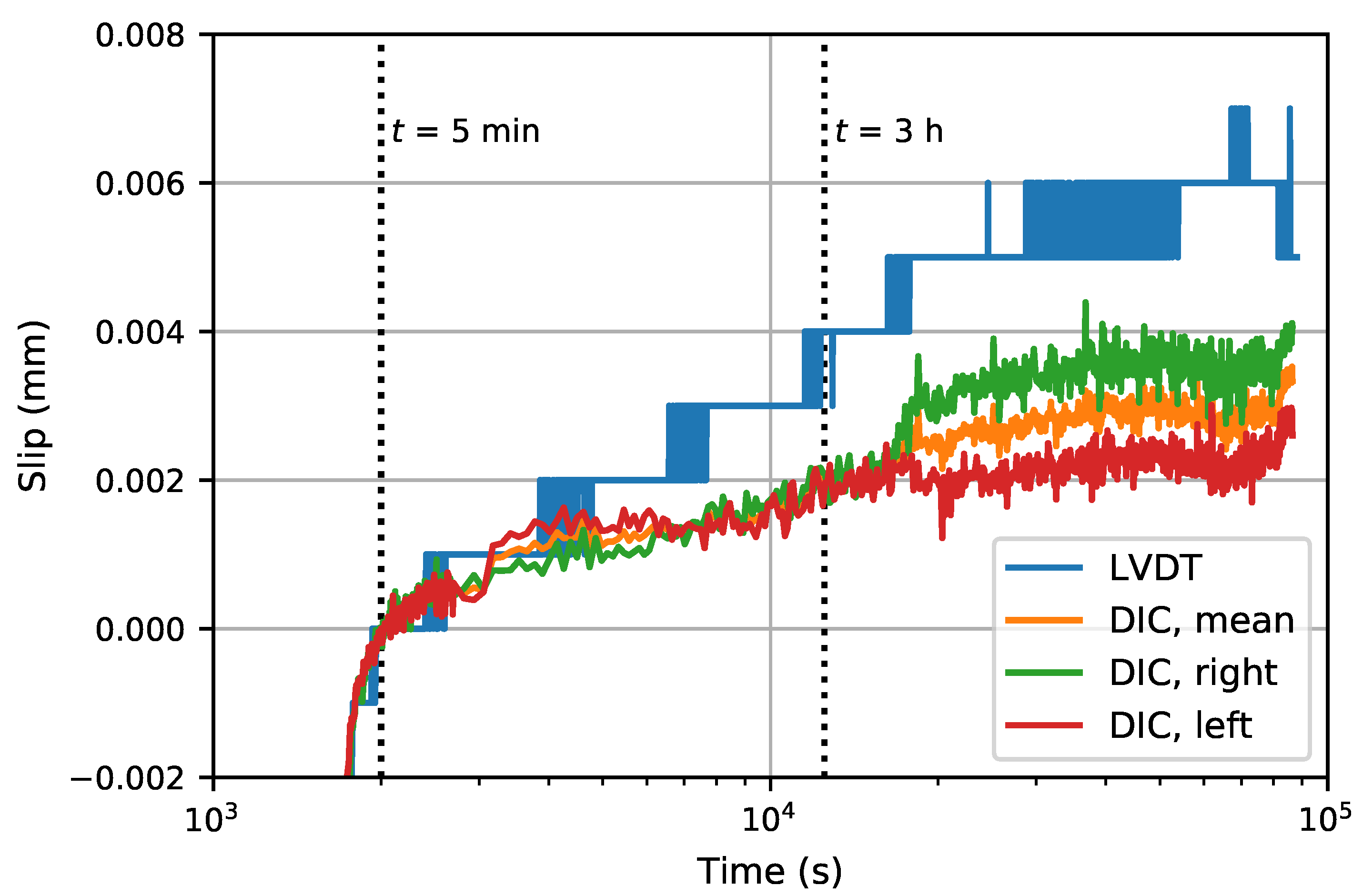
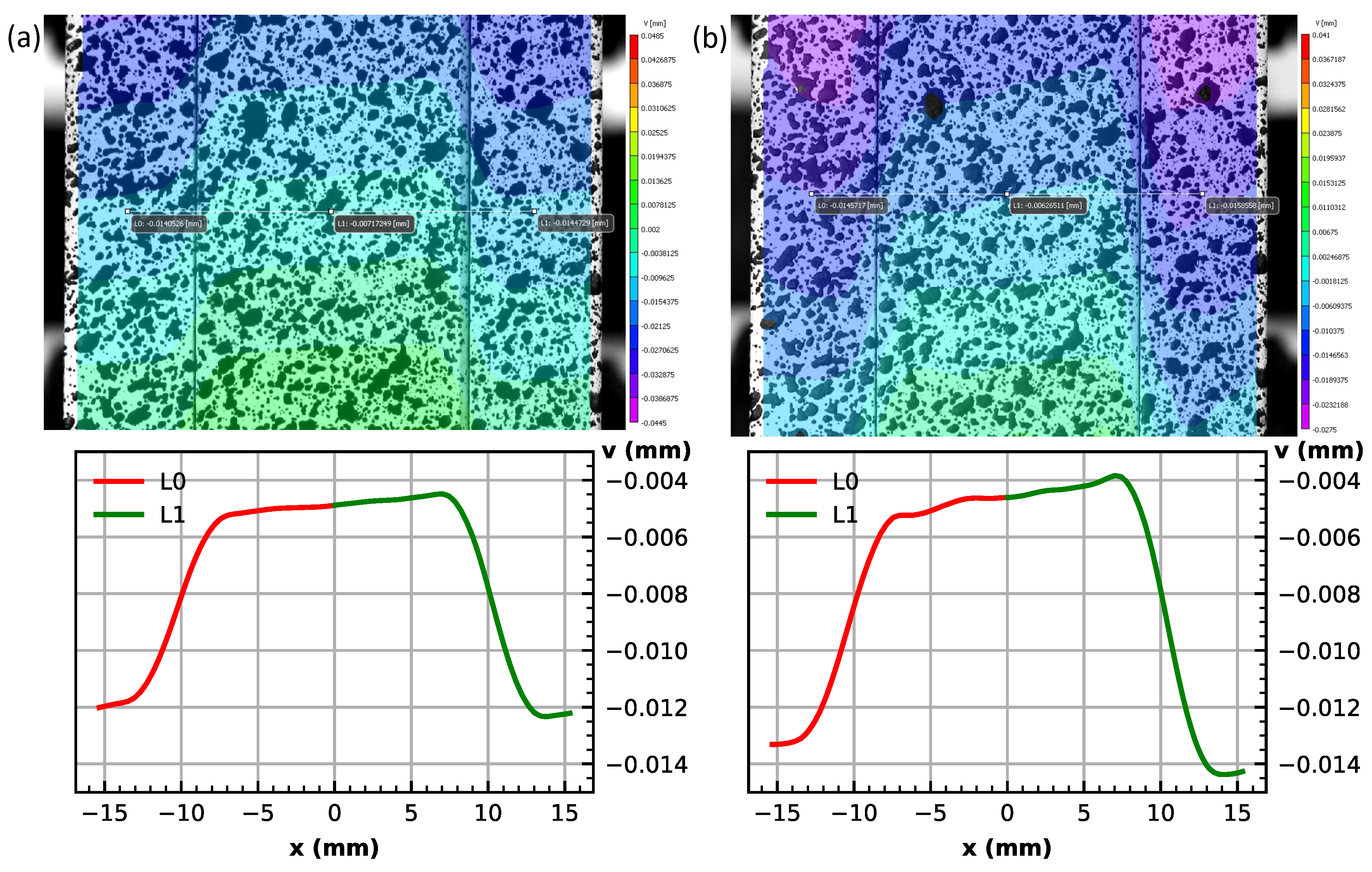
4.2. DIC Measurement

DIC measurements, instead of a unique signal, consist of the displacement field in the ROI at different stages along the test. At each displacement state, different measurements can be taken within the analyzed area. In particular, it is possible to measure the difference in displacements between the center points on the cover plates with respect to the center point on the inner plate, at the middle position between the bolts, as it is required by the standard of steel structures. In this case, it is easy to obtain independent measurements at each side of the inner plate, contrary to the case when using an LVDT.
In order to obtain the relative slip between the inner plate and the cover plates, we focus on the field of vertical displacements, as the specimen was vertically aligned in the test. The delayed slip during the time from the first five minutes of sustained force to three hours can be obtained by comparing the absolute displacement accumulated at both stages from the test beginning. This information is presented in Figure 9. The left subfigure corresponds to the time of five minutes and the right one to the time of three hours. Within each one, an image of the complete displacement field is shown in the first place. In the second place, a graph is presented that shows the displacement distribution along the horizontal line set at the original position of the reference points, where L0 and L1 correspond to the left and right sides, respectively.
In this graph, the vertical axis shows the total vertical displacement developed along that line until the corresponding stage. The origin of the axis is arbitrary in this case. Regarding the x-axis, its origin corresponds to the center point on the inner plate, so the abscissa values of −15 mm and 15 mm correspond to the center points on the left and right cover plates, respectively. Therefore, the difference in the displacement value between these points is the relative slip at each stage, s 5 m i n and s 3 h . For example, the relative slip between the inner plate and the left cover plate was 7.1 μm at five minutes and 8.7 μm at three hours, with the values rounded to the corresponding precision level. As a result, the total slip difference during the delayed slip test is 1.6 μm. The results of both slip measurements and their mean value are as follows:
Δ s DIC , left = 1.6   μ m
Δ s DIC , right = 2.3   μ m
Δ s DIC , mean = 1.9   μ m
By this measuring method, the result of mean slip displacement is at the limit of the tolerance Δ s tol . Attending only to this mean slip value, which is the magnitude comparable to the measurement given by the LVDT, the result of the delayed slip test would meet the conditions established by the standard, and no more tests would be necessary. However, as the DIC method has allowed us to check the independent slips of both cover plates, extended creep tests should be performed afterward due to the value obtained for the right cover plate, which was greater than 2 μ m . Furthermore, the measurements have an uncertainty of ± 0.4   μ m , so satisfactory results should be equal to 1.6   μ m or less.
Similarly to the procedure followed to read the slip values given by Equations (2) and (3) from Figure 9, a continuous slip–time curve can be obtained based on the relative displacement between the steel plates on each picture taken along the test duration, for both cover plates. The mean slip displacement is obtained as the average of both curves, which is the one directly comparable with the LVDT displacement signal shown in Figure 8. All these curves are compared in Figure 10, again setting the origin of the slip at 5 min under constant load.
Regarding the curves obtained by the DIC method, they also present noise, like in the case of the LVDT, but its maximum amplitude is under 1 μ m thanks to the better precision and resolution of this technique. This noise is due to different error sources like subtle differences in lighting or vibrations of the equipment, performance of the numerical algorithm, etc. The noise seems to increase beyond the time of 3 h, but that effect is produced by the logarithmic scale, which compresses many hours in a length that previously corresponded to a few hours or minutes under 104 s. The right and left DIC curves are very close to each other up to a time around 4 h when they separate a short distance that is kept until the end of the test, which points to a dissimilar slip process at each side of the inner plate. In this case, the inner plate can be pulling the left cover plate with it. Comparing DIC with the LVDT, the four curves follow the same path until shortly after t = 5 min. From then on, the four curves continue with an increasing tendency but the slip measured by the LVDT grows faster. This observed difference, apart from the already given explanation about the precision of the measurements, can also be related to the fact that the LVDT is fixed on the specimen, which is undergoing movements and deformations, which can alter the result given by the device. This does not happen with the DIC method, where the measurement is computed from the instantaneous displacement field capture from a fixed point independent of the specimen.
The precision that can be achieved and the fact that it is a contactless technique, avoiding many inconveniences of the setup with traditional measuring tools, justifies the use of the DIC method. But those are just two advantages that it presents. One of the strengths of the method lies in that it provides a full-field measurement, so the obtained information is not limited to a relative displacement between two points. The displacement fields in Figure 9 also show the deformation experienced by the plates besides their relative slip. The high normal force applied by the bolts on the contact surfaces makes the slip only happen under a very high shear stress. This creates a strain gradient in the thickness of the plates until a certain depth at which the vertical displacement becomes approximately constant within the core region of the plates. The analysis of this aspect would be necessary in cases where an unwanted plastic strain could be expected due to this stress component.
However, with respect to the displacement gradients shown in the figure, it is necessary to clarify that the implemented method used by the software considers that the ROI corresponds to a continuous surface of a material. Therefore, it performs a continuous interpolation of displacements between the three layers of the bolted assembly, so the value of the strain localized near the contacts of the plates mixes both the real deformation of the material due to the friction force and the slip movement between the plates. In reality, displacement discontinuities should also appear at the x positions of −10 mm and 10 mm [36]. Nevertheless, the reference points for the standard measurement of the slip are far from the region affected by this interpolation method, and their displacement value is correct.

5. Conclusions

The study presented here analyzes the problem of measuring, with the necessary accuracy, the relative displacements between steel plates in a bolted joint to check the requirement of the standard EN 1090-2:2018 for delayed slips. In a test under a given constant force, the admissible slip during the first three hours must not be greater than Δ s tol = 2 μ m . The present article emphasizes that this strict displacement tolerance is under the measuring precision of most instruments, such as many LVDTs, even if their resolution is 1 μ m . The novelty of the present work is to introduce the optical method of Digital Image Correlation as an alternative to obtain a better approximation of the real displacement in this type of test.
In the first case, measuring the different slips considered by the standard can be physically very difficult with this type of device due to the limited space where they have to be fixed, together with various auxiliary elements. Due to this reason, only the mean slip of the inner plate with respect to both cover plates could be measured. Another limitation is the possible need for a minimum measuring range of the LVDT, a case in which deviations due to its worse precision level could be higher than the admissible tolerance of the displacement to be measured. This is also the situation in the experimental test that has been performed.
On the contrary, the DIC contactless technique, as a full-field method, provides a clean measurement of any desired displacement within the area selected as the Region of Interest. Therefore, it permits measuring the independent slip in each contact surface. Another advantage is that the experimental setup is relatively simple and the equipment is affordable. Finally, better measuring resolutions, and correspondingly better precisions, can be achieved, which makes this method suitable for the practical application treated here.
In this article, a comparison has been made between both measuring methods. The measurement provided by an LVDT with a 10 mm range and a precision of 3 μ m is compared with a DIC computation where the pixel width was equivalent to 39 μ m , and 100-pixel subdivisions were taken, thereby setting its precision to 0.4   μ m . The results show a difference of around 2 μ m between them. The measurement of the LVDT was double the allowed tolerance, while the measurement by the DIC method was around that value. Although the appropriate conclusion from the obtained results of this test in particular would be that it is necessary to perform extended creep tests, using one measuring method or the other can suppose whether the requirement of the standard is satisfied or not.

Author Contributions

Conceptualization, G.R.; methodology, G.R. and X.Z.; formal analysis, J.J.O. and K.P.; investigation, J.J.O., K.P., X.Z. and G.R.; resources, G.R.; writing—original draft preparation, J.J.O.; writing—review and editing, G.R., X.Z. and K.P.; visualization, J.J.O. and K.P.; funding acquisition, G.R. All authors have read and agreed to the published version of the manuscript.

Funding

This research was funded by the Ministerio de Ciencia e Innovación, Spain, through grant PID2019–110928RB–C31, and by the Universidad de Castilla-La Mancha, Spain, and the Fondo Europeo de Desarrollo Regional through grant 2022-GRIN-34124.

Data Availability Statement

The data presented in this study are available on request from the corresponding author.

Conflicts of Interest

The authors declare no conflicts of interest.

References

  1. Connor, J.J.; Faraji, S. Fundamentals of Structural Engineering, 2nd ed.; Springer: Cham, Switzerland, 2016. [Google Scholar] [CrossRef]
  2. EN 1090-2:2018; Execution of Steel Structures and Aluminium Structures—Part 2: Technical Requirements for Steel Structures. CEN: Brussels, Belgium, 2018.
  3. Stranghöner, N.; Afzali, N.; de Vries, P.; Glienke, R.; Ebert, A. Optimization of the test procedure for slip factor tests according to EN 1090-2. Steel Constr. 2017, 10, 267–281. [Google Scholar] [CrossRef]
  4. Cruz, A.; Simões, R.; Alves, R. Slip factor in slip resistant joints with high strength steel. J. Constr. Steel Res. 2012, 70, 280–288. [Google Scholar] [CrossRef]
  5. Chen, G.; Zhang, B.; Liu, P.; Ding, H. An Adaptive Analog Circuit for LVDT’s Nanometer Measurement without Losing Sensitivity and Range. IEEE Sens. J. 2015, 15, 2248–2254. [Google Scholar] [CrossRef]
  6. Felipe-Sesé, L.; Molina-Viedma, A.J.; Pastor-Cintas, M.; López-Alba, E.; Díaz, F.A. Exploiting phase-based motion magnification for the measurement of subtle 3D deformation maps with FP+2D-DIC. Measurement 2022, 195, 111122. [Google Scholar] [CrossRef]
  7. Shao, Y.; Li, L.; Li, J.; An, S.; Hao, H. Target-free 3D tiny structural vibration measurement based on deep learning and motion magnification. J. Sound Vib. 2022, 538, 117244. [Google Scholar] [CrossRef]
  8. Scislo, L. Single-Point and Surface Quality Assessment Algorithm in Continuous Production with the Use of 3D Laser Doppler Scanning Vibrometry System. Sensors 2023, 23, 1263. [Google Scholar] [CrossRef]
  9. Peters, W.H.; Ranson, W.F. Digital imaging techniques in experimental stress-analysis. Opt. Eng. 1982, 21, 427–431. [Google Scholar] [CrossRef]
  10. Sutton, M.A.; Wolters, W.J.; Peters, W.H.; Ranson, W.F.; McNeill, S.R. Determination of displacements using an improved digital correlation method. Image Vis. Comput. 1983, 1, 133–139. [Google Scholar] [CrossRef]
  11. Chu, T.C.; Ranson, W.F.; Sutton, M.A.; Peters, W.H. Applications of Digital-Image-Correlation techniques to experimental mechanics. Exp. Mech. 1985, 25, 232–244. [Google Scholar] [CrossRef]
  12. Sutton, M.A.; Orteu, J.J.; Schreier, H. Image Correlation for Shape, Motion and Deformation Measurements. Basic Concepts, Theory and Applications; Springer: Berlin/Heidelberg, Germany, 2009. [Google Scholar]
  13. Gencturk, B.; Hossain, K.; Kapadia, A.; Labib, E.; Mo, Y.L. Use of digital image correlation technique in full-scale testing of prestressed concrete structures. Measurement 2014, 47, 505–515. [Google Scholar] [CrossRef]
  14. Hild, F.; Roux, S. Comparison of local and global approaches to Digital Image Correlation. Exp. Mech. 2012, 52, 1503–1519. [Google Scholar] [CrossRef]
  15. Pan, K.; Yu, R.C.; Ruiz, G.; Zhang, X.X.; Wu, Z.; de la Rosa, A. The propagation speed of multiple dynamic cracks in fiber-reinforced cement-based composites measured using DIC. Cem. Concr. Compos. 2021, 122, 104140. [Google Scholar] [CrossRef]
  16. Lu, H.; Cary, P.D. Deformation measurements by digital image correlation: Implementation of a second-order displacement gradient. Exp. Mech. 2000, 40, 393–400. [Google Scholar] [CrossRef]
  17. Reu, P.L. A realistic error budget for two dimension Digital Image Correlation. In Advancement of Optical Methods in Experimental Mechanics; Conference Proceedings of the Society for Experimental Mechanics Series; Jin, H., Yoshida, S., Lamberti, L., Lin, M.T., Eds.; Springer: Cham, Switzerland, 2016; Volume 3, Chapter 24; pp. 189–193. [Google Scholar] [CrossRef]
  18. Réthoré, J.; Hild, F.; Roux, S. Shear-band capturing using a multiscale extended digital image correlation technique. Comput. Methods Appl. Mech. Eng. 2007, 196, 5016–5030. [Google Scholar] [CrossRef]
  19. de Crevoisier, J.; Swiergiel, N.; Champaney, L.; Hild, F. Identification of in situ frictional properties of bolted assemblies with digital image correlation. Exp. Mech. 2012, 52, 561–572. [Google Scholar] [CrossRef]
  20. Lacey, A.W.; Chen, W.; Hao, H.; Bi, K. Experimental and numerical study of the slip factor for G350-steel bolted connections. J. Constr. Steel Res. 2019, 158, 576–590. [Google Scholar] [CrossRef]
  21. ISO 5725-1:1994; Accuracy (Trueness and Precision) of Measurement Methods and Results—Part 1: General Principles and Definitions. ISO: Geneva, Switzerland, 2018.
  22. Menditto, A.; Patriarca, M.; Magnusson, B. Understanding the meaning of accuracy, trueness and precision. Accredit. Qual. Assur. 2007, 12, 45–47. [Google Scholar] [CrossRef]
  23. Jones, E.M.C.; Iadicola, M.A. (Eds.) A Good Practices Guide for Digital Image Correlation; International Digital Image Correlation Society: Boston, MA, USA, 2018. [Google Scholar] [CrossRef]
  24. Tian, Q.; Huhns, M.N. Algorithms for subpixel registration. Comput. Vis. Graph. Image Process. 1986, 35, 220–233. [Google Scholar] [CrossRef]
  25. Schreier, H.W.; Sutton, M.A. Systematic errors in digital image correlation due to undermatched subset shape functions. Exp. Mech. 2002, 42, 303–310. [Google Scholar] [CrossRef]
  26. Luu, L.; Wang, Z.; Vo, M.; Hoang, T.; Ma, J. Accuracy enhancement of digital image correlation with B-spline interpolation. Opt. Lett. 2011, 36, 3070–3072. [Google Scholar] [CrossRef]
  27. HajiRassouliha, A.; Taberner, A.J.; Nash, M.P.; Nielsen, P.M.F. Subpixel phase-based image registration using Savitzky-Golay differentiators in gradient-correlation. Comput. Vis. Image Underst. 2018, 170, 28–39. [Google Scholar] [CrossRef]
  28. Barranger, Y.; Doumalin, P.; Dupré, J.C.; Germaneau, A. Digital Image Correlation accuracy: Influence of kind of speckle and recording setup. In Proceedings of the ICEM 14: 14th International Conference on Experimental Mechanics, Poitiers, France, 4–9 July 2010; EPJ Web of Conferences. Bremand, F., Ed.; EDP Sciences: Les Ulis, France, 2010; Volume 6, p. 31002. [Google Scholar] [CrossRef]
  29. Bomarito, G.F.; Hochhalter, J.D.; Ruggles, T.J.; Cannon, A.H. Increasing accuracy and precision of digital image correlation through pattern optimization. Opt. Lasers Eng. 2017, 91, 73–85. [Google Scholar] [CrossRef]
  30. Pan, B.; Yu, L.; Wu, D. High-Accuracy 2D Digital Image Correlation Measurements with Bilateral Telecentric Lenses: Error Analysis and Experimental Verification. Exp. Mech. 2013, 53, 1719–1733. [Google Scholar] [CrossRef]
  31. Reis, M.; Adorna, M.; Jirousek, O.; Jung, A. Improving DIC accuracy in experimental setups. Adv. Eng. Mater. 2019, 21, 1900092. [Google Scholar] [CrossRef]
  32. Pan, B.; Li, K. A fast digital image correlation method for deformation measurement. Opt. Lasers Eng. 2011, 49, 841–847. [Google Scholar] [CrossRef]
  33. Pan, B.; Li, K.; Tong, W. Fast, robust and accurate Digital Image Correlation calculation without redundant computations. Exp. Mech. 2013, 53, 1277–1289. [Google Scholar] [CrossRef]
  34. Reu, P.L.; Toussaint, E.; Jones, E.; Bruck, H.A.; Iadicola, M.; Balcaen, R.; Turner, D.Z.; Siebert, T.; Lava, P.; Simonsen, M. DIC Challenge: Developing images and guidelines for evaluating accuracy and resolution of 2D analyses. Exp. Mech. 2018, 58, 1067–1099. [Google Scholar] [CrossRef]
  35. Reu, P.L.; Toussaint, E.; Jones, E.; Bruck, H.; Iadicola, M.; Balcaen, R.; Turner, D.; Siebert, T.; Lava, P.; Simonsen, M.; et al. Update on the 2D-DIC Challenge: Results and Conclusions. In Advancement of Optical Methods & Digital Image Correlation in Experimental Mechanics, Volume 3; Lamberti, L., Lin, M.T., Furlong, C., Sciammarella, C., Reu, P.L., Sutton, M.A., Eds.; Conference Proceedings of the Society for Experimental Mechanics Series; Springer: Berlin/Heidelberg, Germany, 2019; pp. 81–84. [Google Scholar] [CrossRef]
  36. Dupré, J.C.; Doumalin, P.; Husseini, H.A.; Germaneau, A.; Bremand, F. Displacement discontinuity or complex shape of sample: Assessment of accuracy and adaptation of local DIC approach. Strain 2015, 51, 391–404. [Google Scholar] [CrossRef]
Figure 1. Definition of DIC parameters.
Buildings 14 01046 g001
Figure 2. Dimensions of the different plates in mm: (a) inner plate and (b) cover plate.
Buildings 14 01046 g002
Figure 3. Side view of the assembly sketching the measurement of the relative displacement s i in a situation where the inner plate on the right has undergone a slip movement.
Buildings 14 01046 g003
Figure 4. Test configuration: (a) testing machine, (b) instrumented specimen, and (c) detail of the LVDTs and the speckle pattern for DIC.
Buildings 14 01046 g004
Figure 5. Verification of the accuracy of the measurements with the LVDTs.
Buildings 14 01046 g005
Figure 6. Loading course of the delayed slip test, where t f t 0 3 h.
Buildings 14 01046 g006
Figure 7. Force–slip curves to determine F S m .
Buildings 14 01046 g007
Figure 8. Slip–time curve provided by the LVDT.
Buildings 14 01046 g008
Figure 9. Vertical displacement fields and displacement distributions between reference points: (a) at five minutes and (b) at three hours.
Buildings 14 01046 g009
Figure 10. Comparison of the slip–time curves of the LVDT and the DIC method.
Buildings 14 01046 g010
Table 1. Precision of LVDTs, in mm, for different ranges.
PrecisionFull Range (± Full Scale) [mm]
1 (±0.5)2 (±1)5 (±2.5)10 (±5)
0.10%0.0010.0020.0050.01
0.25%0.00250.0050.01250.025
0.50%0.0050.010.0250.05
Disclaimer/Publisher’s Note: The statements, opinions and data contained in all publications are solely those of the individual author(s) and contributor(s) and not of MDPI and/or the editor(s). MDPI and/or the editor(s) disclaim responsibility for any injury to people or property resulting from any ideas, methods, instructions or products referred to in the content.

