Strategies for Mitigating Urban Residential Carbon Emissions: A System Dynamics Analysis of Kunming, China

Abstract

To effectively combat environmental challenges, it is necessary to evaluate urban residential building carbon emissions and implement energy-efficient, emission-reducing strategies. The lack of a specialized carbon emission monitoring system complicates merging macro- and micro-level analyses to forecast urban residential emissions accurately. This study employs a system dynamics (SD) model to examine the influence of social, economic, energy, and environmental factors on carbon emissions in urban residences in Kunming, China. The SD model forecasts household carbon emissions from 2022 to 2030 and establishes three scenarios: a low-carbon scenario (LCS), a medium low-carbon scenario (MLCS), and a high low-carbon scenario (HLCS) to assess emission reduction potentials. It predicts emissions will climb to 4.108 million tons by 2030, significantly surpassing the 2014 baseline, with economic growth, urbanization, residential energy consumption, and housing investment as key drivers. To curb emissions, the study suggests enhancing low-carbon awareness, altering energy sources, promoting research and development investment, and expanding green areas. The scenarios indicate a 5.1% to 16.1% emission reduction by 2030 compared to the baseline. The study recommends an 8.3% to 11.4% reduction in MLCS as a practical short-term target for managing urban residential emissions, offering a valuable SD approach for optimizing carbon strategies and aiding low-carbon development.

1. Introduction

The sixth assessment report of the Intergovernmental Panel on Climate Change (IPCC) highlights the significant contribution of urban areas to global carbon emissions [1]. Currently, over half of the global population resides in urban regions, which are responsible for approximately 71–76% of global end-use energy consumption and 67–76% of CO₂ emissions attributable to energy use in cities [2]. This trend suggests an ongoing and likely increase in energy consumption and carbon emissions from residential buildings, particularly considering the growing urban population.

Residential carbon emissions can be categorized into five key phases: manufacturing of building materials, construction, usage, maintenance, and finally, demolition and disposal [3]. For instance, in 2020, the residential building sector of China accounted for 45.5% of the total national energy consumption and 50.9% of its carbon emissions. The production of building materials and building operation phases are the most significant contributors, accounting for 28.2% and 21.7% of emissions, respectively [4]. Notably, the operational phase tends to increase its emissions proportionally over time, eventually becoming the dominant source over the lifecycle of the building [5]. Therefore, it is crucial to study the carbon emissions of urban residential buildings during the use phase and, on this basis, formulate energy-saving and emission reduction strategies for urban residential buildings during the operation phase to reduce carbon emissions.

A deeper look shows that various macro factors, including urbanization, demographics, climate parameters, economic development, and energy consumption, have been identified as significant drivers of emissions from urban residential buildings. Studies, such as those by Burleyson et al. [6], Wang et al. [7], and Huo et al. [8], highlight how urbanization affects household energy patterns and thereby impacts carbon emissions, with noticeable regional variations. Climate conditions also play a crucial role in influencing construction intensity and energy consumption [9,10].

On the micro-level, research presents a more nuanced picture. There is evidence suggesting that higher household incomes may lead to increased energy consumption [11,12], while other studies propose that wealthier households tend to adopt energy-saving practices [13,14]. Notably, household energy use patterns in China differ significantly between urban and rural areas and across different regions [15], depending on things like building types, heating systems, population density, and educational levels [16,17]. However, much of the existing research tends to isolate these factors, overlooking their interconnected and cumulative effects.

In framing emission reduction strategies, it becomes clear that variations in lifestyle and usage patterns can lead to significant disparities in household energy consumption, with differences of up to 300% [18]. This highlights the importance of considering both micro- and macro-level factors, like income, consumption habits, urban expansion, and population dynamics [19,20], in designing low-carbon pathways. Additionally, building design and usage patterns have important influences on carbon abatement outcomes. For instance, regarding heating mode selection, centralized heating entails higher energy use [21]. However, after accounting for per capita metrics, centralized systems demonstrate superior energy savings over distributed heating alternatives. To address these complexities, some scholars have incorporated policy effects like carbon trading into their analyses [22,23].

In this context, Kunming, as Yunnan Province’s political, economic, and cultural center, emerges as a focal point in China’s low-carbon initiative. Despite setting explicit targets for carbon emission reduction, Kunming faces ongoing challenges with high residential carbon emissions, exacerbated by its growing population and economic growth. Current research on the residential carbon footprint of Kunming predominantly adopts a static approach, neglecting the dynamic evolution of emissions and the underlying mechanisms that drive these changes. This study proposes the development of a system dynamics (SD) model to forecast future emission patterns dynamically, delving into the intricate interplay between various factors—economy, society, energy, and environment—at both macro- and micro-levels. This approach marks a departure from traditional static analysis, highlighting the dynamic interactions within complex systems and offering fresh insights into the mechanisms underlying residential carbon emission trends. Such insights are crucial for enhancing the accuracy of emission predictions and the efficacy of emission reduction strategies. Moreover, this research is poised to inform policy formulation, providing a solid foundation for crafting low-carbon development strategies in Kunming and beyond, thereby underscoring its significance for informed planning and policymaking.

2. Methodology

2.1. Research Framework

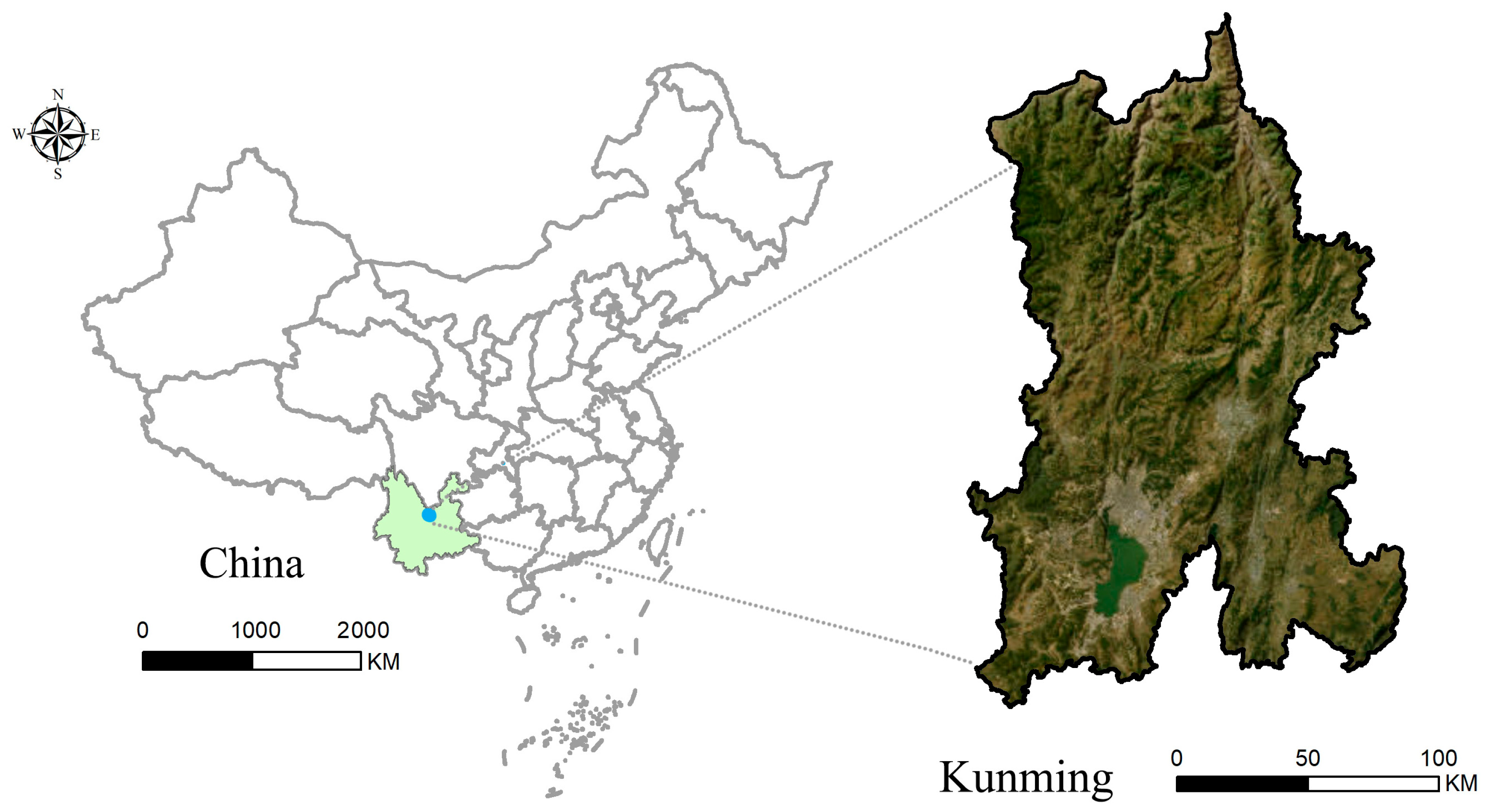
To construct an SD model to simulate the residential carbon emissions system in Kunming, China, this study adhered to the methodology illustrated in Figure 1. Initially, it delineated the boundaries of the system to match the research scope, pinpointed crucial factors within the residential carbon emissions framework, and explained the interrelationships among these factors. Subsequently, feedback loops among subsystem variables were established as the foundation for crafting both the causal loop diagram and the system flow diagram. To complete the construction of the model, this stage involved creating system equations using database data and then conducting rigorous testing and calibration. The next phase entailed devising four experimental scenarios: the baseline, low-carbon scenario (LCS), medium low-carbon scenario (MLCS), and high low-carbon scenario (HLCS), each reflecting the status of Kunming and the long-term strategic vision of the government. Finally, the study executed these scenarios, analyzed the simulation outcomes, and derived relevant conclusions.

2.2. Study Area

Kunming, the capital of southwest China (Figure 2), is experiencing rapid urbanization. In 2021, its population reached 8,873,500, with an urbanization rate of 79.6%, and this urban expansion has led to a residential area growth of 105 million square meters [24]. Kunming has a plateau monsoon climate at an elevation of around 2000 m. It experiences ample sunshine year-round, substantial diurnal temperature variations yet minor seasonal differences, four distinct seasons without frigid winters or sweltering summers [25], an annual average temperature of 16.5 °C, as well as adequate and suitable sunlight exposure, which has earned it the nickname “Spring City” [26]. The energy consumption patterns of the city are heavily influenced by its climate, which is characterized by mild winters and cool summers. This climate allows for natural ventilation in summer and minimal heating in winter, with electricity, rather than air conditioning, being the primary energy consumer.

The geographical location and climatic conditions of Kunming have shaped a distinctive energy consumption pattern and residential building energy use. As a national low-carbon pilot city of China, Kunming has made notable early achievements in reducing carbon emissions and has established ambitious objectives for the future. This achievement underlines the necessity for well-thought-out strategies for continued carbon reduction efforts. Moreover, the endeavors in carbon reduction in Kunming offer invaluable insights for other Chinese cities with analogous climates, such as Guiyang and Zunyi, that are on a similar low-carbon journey. However, despite the benefits derived from its geographic, climatic, and policy framework, Kunming faces challenges due to an increasing demand for energy-intensive home appliances and rapid urbanization, which have escalated domestic energy usage. This situation highlights the critical need for a detailed investigation into the urban residential carbon emissions in Kunming. Such an analysis is essential to crafting effective local low-carbon strategies, aiming to achieve broader zero-carbon targets.

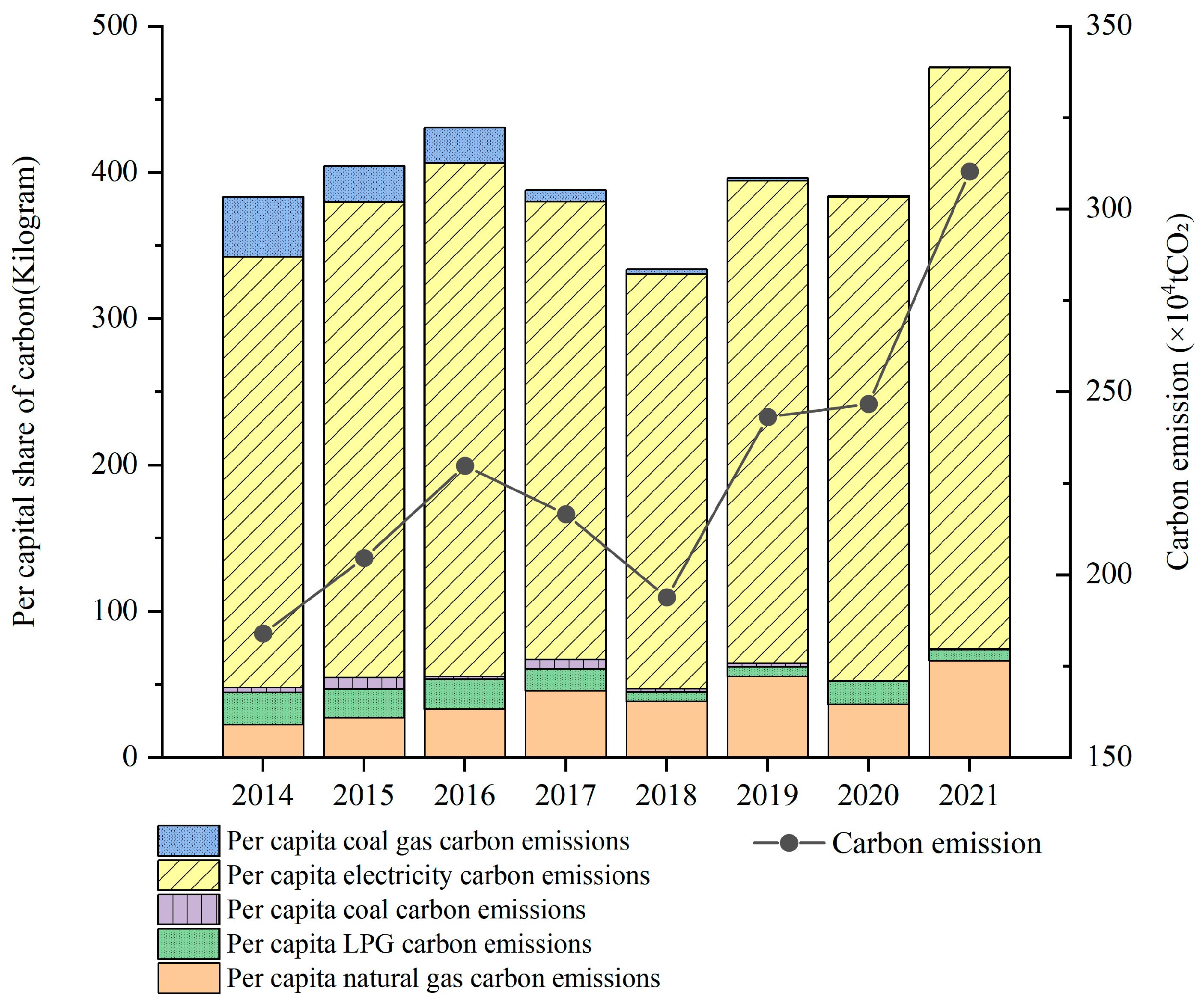
2.3. Carbon Emission Accounting Method

In the building industry of China, the lack of a dedicated carbon emission monitoring system necessitates the use of various computational techniques for carbon emission estimation. Among these, micro-methods, notably the computer simulation technique and actual measurement technique, are commonly employed. The actual measurement method is apt for industries with significant emissions and intricate emission characteristics [27], and computer simulation predominantly focuses on micro-level studies of specific systems and processes, often struggling with the complexity of macro-level objects [28,29]. Therefore, life cycle assessment (LCA) methods can be used to provide in-depth analysis at the individual level and scale up to assess larger systems. However, despite its comprehensive approach, LCA is constrained by the challenges of data acquisition and workload [30,31].

Alternatively, the IPCC carbon emission factor method is widely embraced in the construction sector for its simplicity, accessibility of data, and broad applicability [32,33]. It adeptly addresses both macro- and micro-level analysis requirements. This study adopts the IPCC method for macro-level carbon emission assessment, utilizing the statistical data available in the regional yearbooks of Kunming. The IPCC coefficients are calculated using Equation (1):

$$C=\sum E_{\mathit{i}}\times {\mu }_{\mathit{i}}$$

(1)

where C denotes total carbon emissions; E_i denotes the consumption of the ith energy source; and μ_i denotes the carbon emission factor of the ith energy source.

As shown in

Table 1. Standard coal coefficient of various energy sources (reference value). [34,35].

Energy Source	Average Status Heat Generation	Conversion Factor of Standard Coal
Raw coal	20,934 kJ/kg (5000 kcal/kg)	0.7143 kgce/kg
Petroleum	38,979 kJ/kg (9310 kcal/kg)	1.3300 kgce/m3
Liquefied petroleum gas	50,242 kJ/kg (12,000 kcal/kg)	1.7143 kgce/kg
Coke oven gas	18,003 kJ/kg (4300 kcal/kg)	0.6143 kgce/m3

, data from the Kunming Statistical Yearbook [34] and Energy Statistical Yearbook (2014–2021) [35] form the basis of this study analysis, with conversion coefficients for various energy sources normalized to standard coal equivalents as per the 2020 China Energy Statistical Yearbook. The electricity emission factor is sourced from [36,37], and this study applied an emission factor of 0.5271 kg CO₂/kWh for Kunming.

Figure 3 illustrates the trend in urban residential carbon emissions in Kunming from 2014 to 2021, highlighting a continual upward trajectory from 1.839 million tons to 3.102 million tons. This represents an average annual growth rate of 18.6%. The escalation in emissions is closely linked to the enhancement of living standards and the rapid pace of urbanization. Notably, a decline in emissions was observed in 2017 and 2018, aligning with significant changes in the city’s energy infrastructure. This period marked the extensive substitution of piped artificial gas with natural gas, signaling a transition to more environmentally friendly energy sources. Despite the adoption of natural gas, a cleaner energy alternative, aggregate carbon emissions continued to escalate, driven by factors such as population growth, heightened living standards, and an increasing demand for energy services.

The findings also indicate a shift in the composition of carbon emission sources. Prior to 2017, gas and electricity constituted about 90% of the total residential carbon emissions in Kunming. After 2018, the share of natural gas and electricity exceeded 95%, highlighting a continuous decline in emissions from coal, liquefied petroleum gas (LPG), and gas. This trend underscores the importance of energy structure in emission reduction strategies, although the ongoing rise in emissions suggests that improvements in energy structure alone may not fully offset the environmental impact of other factors driving increased energy demand.

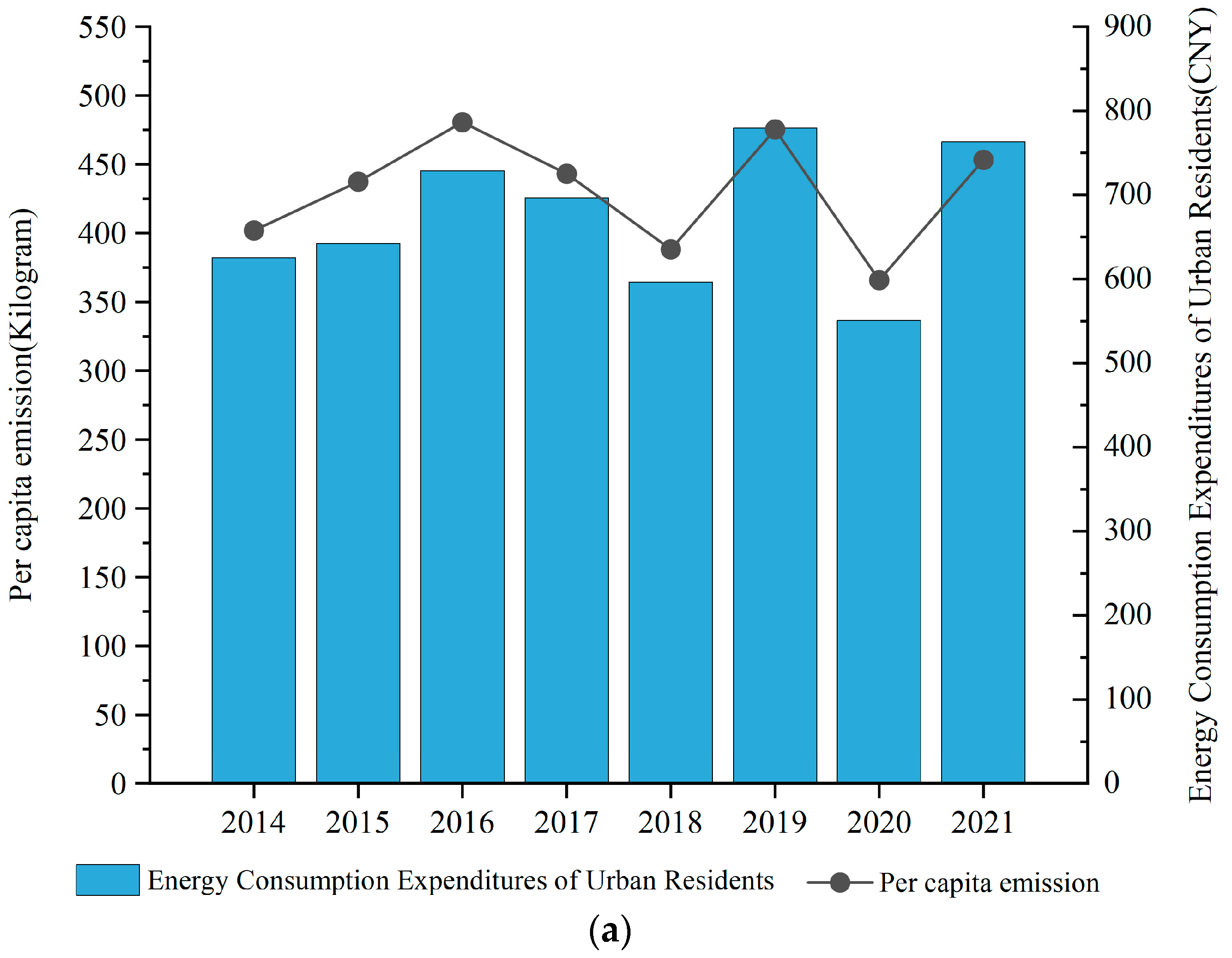
2.4. Influencing Factors

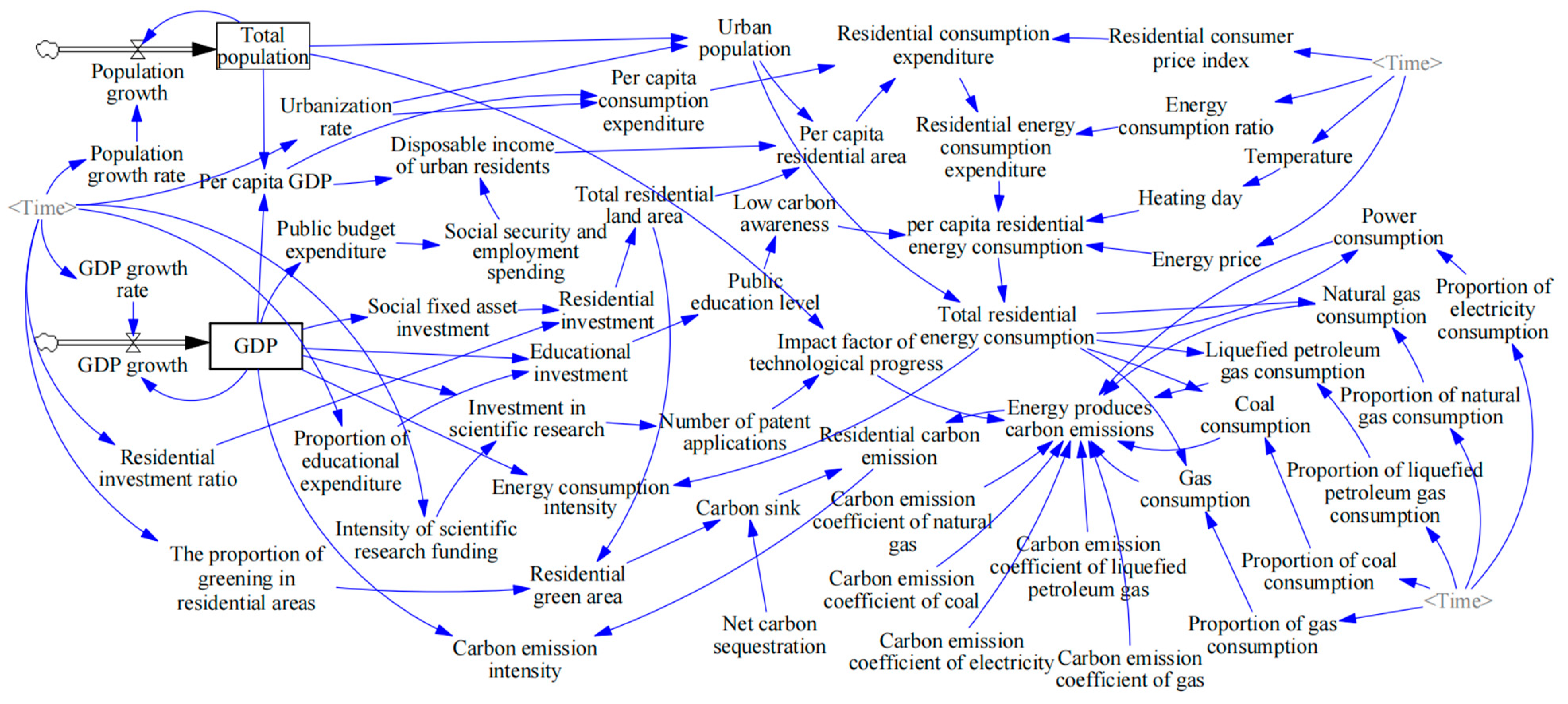
In this study, the SD model was used to conduct an in-depth analysis of carbon emissions from residential buildings. Central to this analysis is the identification of key influencing factors. By sorting and summarizing the literature [8,9,10], a preliminary set of influencing factors was determined. Grey correlation analysis [38] is then employed to further refine and validate these factors. The grey correlation analysis method is mainly used to judge the degree of correlation through the similarity of the trend of the data series, identify the advantages and disadvantages of the judged object, and does not reflect the absolute level [39]. This technique directly calculates using original data without normalization, thus offering strong reliability [40]. By calculating the grey correlation coefficients between diverse factors and carbon emissions, the correlation between each pair can be determined. The results reveal that only residential floor area completed, urban road area per capita, and annual technology contract transaction amount have low correlations, while the grey correlations of other factors exceed 0.7, indicating strong correlations [40,41]. Therefore, this meticulous approach enables the identification of 22 distinct influencing factors, categorized across four subsystems, which are detailed in Appendix A. Prominent among these are the energy consumption expenditures of residents, energy prices, and heating degree days (Figure 4). Each of these factors plays a significant role in impacting carbon emissions. A significant positive correlation exists between Figure 4a,c, revealing the energy consumption of residents and heating degree days as key drivers of carbon emissions. Figure 4b shows energy prices and per capita emissions negatively correlating short-term; however, long-term trends demonstrate decoupling between the two. This decoupling suggests energy price reforms alone have limited efficacy to improve efficiency and mitigate emissions. Therefore, a combination of other regulatory, technical, and economic policy tools is necessary to effectively achieve the set carbon reduction targets.

2.5. Model Building

Forrester invented SD modeling in 1956, which uses structural function analysis based on computer simulation technology to address complex dynamic feedback systems [42]. Combining cybernetics, information theory, and system theory, SD modeling is a way to look at problems in social, economic, ecological, and other complex systems that are dynamic, nonlinear, and have feedback at more than one level. Recent applications [43,44,45] in urban energy consumption and building carbon dioxide emissions have been noted. Notably, Murray et al. [46] and Liu et al. [47] utilized this methodology for analyzing energy usage and carbon emissions in Changsha City, underscoring its utility in supporting policy decision-making by unraveling the complex mechanisms driving building carbon emissions. Future expansions of this model could encompass a broader range of influencing factors, improved spatial and temporal resolution, and integration with statistical and econometric models for enhanced accuracy. However, research on building carbon emissions using this approach remains relatively limited.

This research conducts a thorough analysis of the intricate framework underlying residential carbon emissions through the lens of SD. It aims to unravel the multitude of factors that drive residential carbon emissions and investigates their interconnections. Identifying key variables, the study leverages feedback mechanisms inherent in the subsystems to construct causal loop diagrams and stock flow diagrams. These diagrams elucidate the mechanisms through which each factor impacts residential carbon emissions.

Regression fitting enabled the calibration of the model parameters, allowing for the simulation of the urban residential carbon emissions trajectory of Kunming for the years 2022–2030. This simulation process is not static; it involves meticulous adjustments to the parameters and influencing factors to accurately reflect the evolving trends of carbon emissions under a variety of potential scenarios. Subsequently, the article provides a detailed analysis of the most effective mitigation strategies. By changing the parameters and contributing factors of the model, the paper puts forward feasible suggestions for reducing emissions. These recommendations are further substantiated through simulations that project the trends of household carbon emissions under diverse scenarios. The structural framework of the SD model in this study is shown in Figure 5, which provides a visual representation of the model’s complexity and its operational dynamics.

For this study, the temporal boundary spans from 2014 to 2030. Among them, 2014–2021 is the historical benchmark period of the model. Kunming carried out the natural gas replacement project from 2014 to 2017, and the energy structure changed, thus affecting residential carbon emissions. The data in this stage are representative and typical and can provide a basis for the estimation and calibration of model parameters; 2022–2030 is the simulation prediction stage. The year 2030 is a key node in the realization of the carbon peak goal of China, and the selection of this period is helpful to evaluate the low-carbon transformation process of Kunming’s residential sector and provide decision-making reference for formulating relevant policies. From 2014 to 2030, the time span is relatively long, considering the short- and medium-term development trend, which is conducive to a comprehensive analysis of the dynamic effects of various influencing factors. The model operates with an annual time step, offering a detailed yet manageable temporal resolution. Spatially, the model focuses on urban residences within Kunming City, specifically targeting the carbon emissions generated during the use phase of these residences. This spatial boundary ensures that the model remains focused on urban residential emissions while capturing the relevant dynamics within the specified geographical context.

The causal loop diagram (Figure 6) is a key component in this study because it demonstrates how various elements of Kunming’s residential carbon emission system interact and affect one another. This study has categorized this system into four distinct subsystems: economic, social, energy, and environmental. Each subsystem encompasses a set of variables and relationships, which are meticulously analyzed and synthesized to delineate the causal dynamics of residential carbon emissions.

In terms of economic subsystems, the study explores how factors like industry investment and economic growth influence residential carbon emissions, along with the associated feedback loops. For instance, Figure 6a traces the path from gross domestic product (GDP) growth to increased social fixed assets and residential investments, leading to an expansion in the total residential land area and per capita residential area. This expansion correlates with an increase in per capita residential energy consumption and, consequently, total residential energy consumption, which in turn impacts carbon emissions and environmental quality. The feedback loop continues with the costs of carbon reduction influencing GDP. Similarly, GDP boosts educational investment, enhancing public education levels and awareness of low-carbon practices, thereby influencing per capita residential energy consumption and total residential energy consumption, which further affects carbon emissions and environmental quality. Another critical aspect involves GDP driving investment in scientific research, leading to an increase in patent applications and the impact factor of technological progress, which also feeds back into the GDP through its influence on carbon emissions and environmental quality.

The primary causative relationship observed is that economic growth not only stimulates societal development and the expansion of residential areas, contributing to increased carbon emissions from residential houses, but also promotes investments in science and education. These investments, in turn, are instrumental in devising strategies to reduce carbon emissions through various avenues, where modifications in any of the variables can exert a direct influence on others, potentially reducing carbon emissions favorably. This reasoning is also used in the feedback loops shown in Figure 6b–d, which show the social, energy, and environmental subsystems, respectively. This shows a complete way to understand and deal with the changes in Kunming, China, residential carbon emissions.

Creating a stock–flow diagram is an important part of this study because it shows exactly how the different parts of the system are connected logically and how dynamic feedback works. This diagrammatic representation is crucial for facilitating a comprehensive analysis and enabling an effective simulation of the system’s behavior. In the context of the SD model in this study, the flows within the system act as catalysts, triggering changes in the stocks. Figure 7 presents the stock flow diagram specifically for residential carbon emissions. This diagram was created using the knowledge obtained from the causal loop diagram presented in Figure 5. It meticulously maps out the flow of variables and their cumulative impact on the stock of carbon emissions, thereby offering a visual and analytical tool to understand and predict the patterns and trends of carbon emissions in residential settings.

The stock and flow diagram in the SD model serves to depict the interplay and causal connections among variables within a system. Here, stock variables, such as population and GDP, are defined by state equations and illustrated as rectangular boxes. Flow pipes, denoted by arrows or valve symbols, connect flow variables to these stocks, such as the population growth rate and economic growth rate. Feedback loops, which are in turn influenced by a variety of external factors, control the size of these flows. This approach underscores the complex dynamics at play, enabling a deeper understanding of the system’s behavior.

This research adopts three foundational methodologies to craft the equations that determine the initial values and variable parameters, forming the crux of the model under investigation, with comprehensive details provided in Appendix B.

The first method, constant determination, leverages an extensive array of sources, including existing research, the Kunming City Development Strategy Plan [48], and the Kunming City Statistical Yearbook [34], among others. This technique anchors the model in the empirical reality of Kunming, China, ensuring it accurately mirrors the city’s current development trajectory.

Secondly, the study employs table function entries to systematically gather variable data over time, introducing a vital temporal element to the analysis. This approach is instrumental in capturing the dynamic evolution of variables. During the mathematical formulation phase, the study judiciously selects the most fitting function type—whether logarithmic, exponential, or linear—based on data trends and patterns. This careful selection is crucial for precisely depicting the interrelationships among variables.

For addressing complex interactions between variables, especially where multiple independent variables impact a dependent variable amidst a mix of linear and nonlinear relationships, the study turns to regression analysis. This statistical technique allows for an in-depth examination of these intricate dynamics. The Statistical Package for the Social Sciences (SPSS) Statistics 27 software, known for its statistical analysis capabilities, was utilized for this purpose, providing a reliable tool for dissecting and interpreting the multifaceted relationships within the model. To ascertain the reliability of the regression analysis outcomes, a battery of statistical tests was executed using SPSS, with the findings detailed in Appendix B 

Table A1. Equation test data of the SD model.

Equation	The Adjusted R-Squared	DW	Correlation Coefficient	VIF
Social fixed-asset investment	0.821
Public budget expenditure	0.925
Social security and employment expenditure	0.915	2.401	0.963	1
Number of patent applications	0.967	1.432	0.986	1
Public education level	0.869	2.249	0.942	1
Residential land area	0.921	1.609	0.966	1.377
Per capita living area	0.912	1.22	0.961	1.377
Consumption Expenditure per urban resident	0.966	1.1	0.861	1.487
Residential consumption expenditure of urban residents	0.915	2.223	0.966	1.137
Residential energy consumption per capita	0.818	1.313	0.844	1.084
Technological Progress Impact Factor	0.899	2.1	0.977	1

. The reliability was first assessed by evaluating the adjusted R-squared, Durbin–Watson (DW) statistics, and the correlation coefficient between independent and dependent variables. This assessment confirmed the strong fit and explanatory power of the regression model, as evidenced by adjusted R-squared values exceeding 0.8, DW values approximating the optimal 2, and the correlation coefficient close to 1 [49,50]. Following this, the analysis delved into investigating potential multicollinearity among the independent variables. The results, indicated by variance inflation factor (VIF) values below 2, demonstrated the absence of significant multicollinearity [51], thereby affirming the accuracy of the regression analysis.

2.6. Model Validation

To ensure the validity and reliability of the SD model, this study has implemented a series of rigorous testing techniques, including boundary testing, structural testing, and historical testing. These methods are essential for a comprehensive reevaluation and integration of the boundaries and subsystem feedback loops of the model. They help make sure that the equations of the model are correct in showing how different variables are related to each other, that parameter value estimates are based on good evidence, and that the quantitative framework is consistent.

The functionality and structural feasibility of the model have been further evaluated using the Vensim 10.1.2 software, a specialized tool for SD modeling [52]. The capability of this software to operate the model effectively attests to the practicality of the boundary and structure of the model. A pivotal aspect of the model validation process in research is historical testing, which involves comparing the simulation results of the model with historical data. The credibility of the model is reinforced when the discrepancy between these two datasets falls within the acceptable error margin of 15 percent as per SD standards [53].

Table 2. Comparison of historical test values and modeling simulation values.

Year	Total Carbon Emissions (×104 tons)			Total Energy Consumption of Urban Dwellings (×104 kg of Standard Coal)
	Actual Value	Analog Value	Error (%)	Actual Value	Analog Value	Error (%)
2014	183.90	175.79	−4.41	63,860.22	61,367.40	−3.90
2015	204.53	200.36	−2.04	66,060.51	64,953.10	−1.68
2016	229.72	235.12	2.35	73,715.49	75,579.30	2.53
2017	216.53	228.81	5.67	68,773.18	72,669.80	5.67
2018	193.77	200.75	3.60	59,051.58	61,263.10	3.75
2019	243.11	252.94	4.04	75,167.47	78,455.60	4.37
2020	246.66	263.90	6.99	73,286.46	78,509.00	7.13
2021	310.24	298.87	−3.67	94,492.23	91,599.80	−3.06
Year	Per capita Disposable Income of Urban Residents (CNY)			Energy Consumption Expenditure of Urban Residents (CNY)
	Actual Value	Analog Value	Error (%)	Actual Value	Analog Value	Error (%)
2014	31,295	32,603.8	4.18	625.27	657.28	5.12
2015	33,955	34,176.5	0.65	642.27	646.88	0.72
2016	36,739	36,458.7	−0.76	728.59	705.00	−3.24
2017	39,788	40,350.6	1.41	696.61	737.61	5.89
2018	42,988	42,506.7	−1.12	596.19	585.44	−1.80
2019	46,289	50,356.6	8.79	779.43	764.77	−1.88
2020	48,018	46,268.5	−3.64	551.03	553.71	0.49
2021	52,523	48,916.6	−6.87	763.00	718.87	−5.78

demonstrates this aspect by presenting a comparison of four key variables: total residential energy consumption, total residential carbon emissions, per capita disposable income, and energy consumption expenditures. The simulation results for these variables exhibit errors significantly lower than 15 percent, all falling under the 10 percent threshold, thus underscoring the accuracy of the model. Consequently, the model not only passes the historical test but also proves its utility in simulating the regulation of residential carbon emissions in Kunming under various policy scenarios. To evaluate how variations in pivotal parameters influence outcomes, sensitivity analysis was employed, with the findings presented in Appendix B 

Table A2. Sensitivity test results of the SD model (%).

Variable	Increase (10%)	Decrease (−10%)
Urbanization rate	2.5	2.5
Population growth rate	5	0.16
Energy prices	3.8	3.8
Proportion of scientific research expenditure	2.8	2.8
Proportion of educational expenditure	3	3
Greening area ratio	1.3	1.3
Residential investment ratio	1.1	1.1
GDP growth rate	3.3	2.4
Heating days	8.3	8.3
Natural gas consumption	8.55	8.55
Liquefied petroleum gas consumption	1.8	1.8
Coal consumption	0.9	0.9
Electricity consumption	2.26	2.26
Gas consumption	0.44	0.44

. The simulation outcomes reveal a low sensitivity to parameter changes, signifying that the model exhibits robust stability. This characteristic affirms the model’s reliability for conducting scenario simulations, indicating its capacity to provide consistent predictions under varying conditions. This stability is crucial for the model’s application in strategic planning and policy development, allowing for confident use in exploring potential future scenarios and their implications.

3. Results

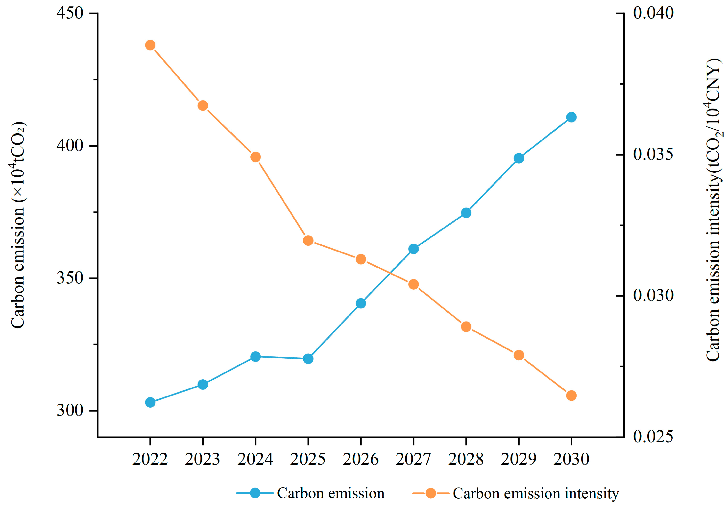
3.1. Simulation Results of the CO₂ Emission Trend

This study uses a carefully constructed simulation model to predict future patterns of carbon emissions and emissions intensity in residential areas of Kunming from 2022 to 2030 (Figure 8). The simulation results indicate a sustained increase in household carbon emissions, mostly due to ongoing urbanization and the improving living standards of its residents. The simulation predicts a significant surge in the household carbon emissions of Kunming, projecting an increase to almost 4.108 million tons by 2030. This value is nearly 2.5 times higher than the baseline level observed in 2014.

Moreover, the model forecasts a substantial decrease in the intensity of carbon emissions from residential sources. It is estimated that by 2025, the emission intensity will reduce to 0.0319 tons/million CNY, which represents an 18.4% decrease from the 2020 level of 0.0392 tons/million CNY. The anticipated reduction is in line with the goal of an 18% reduction, demonstrating Kunming’s commitment to putting effective carbon control measures in place. Nevertheless, it is imperative to recognize the ongoing difficulties in controlling home carbon emissions, even with the introduction of many low-carbon projects. The continuous reduction in carbon emission intensity indicates advancement, but it also emphasizes the requirement for consistent and intensified endeavors in carbon management.

3.2. Simulation of Single-Factor Carbon Emissions

The optimal path to reduce emissions is determined by simulating the four main subsystems—economy, society, energy, and environment—using the scenario analysis method. This analytical approach allows for a detailed examination of how different factors influence various potential trajectories. The adjustments made in these simulations are meticulously outlined in

Table 3. Scenario modeling program settings.

Programmatic	Adjustment Range
Basic program	Keeping the system’s factors constant and progressing smoothly at the pace prior to the x-factor
Option 1	Constant factors in the system, reduce factor x by 1 percentage point
Option 2	Constant factors in the system, increase factor x by 1 percentage point
Option 3	Constant factors in the system, increase factor x by 2 percentage points

, providing insight into the specific strategies implemented.

Simulations in this study indicate that different factors within these subsystems have varying impacts on household carbon emissions, as detailed in Appendix C. The main factors contributing to an increase in carbon emissions include the urbanization rate, the economic growth rate, the residential investment ratio, and the level of residential energy consumption. For instance, a 1% increase in each of these factors leads to annual emission increases of approximately 82,600 tons, 69,800 tons, 3000 tons, and 12,000 tons, respectively, compared to the base scenario. Conversely, factors such as heightened low-carbon awareness, increased scientific research investment, expanded green spaces, optimized energy structures, and rising temperatures serve to inhibit the growth of carbon emissions. Compared to the base scenario, annual emissions will decrease by approximately 17,000 tons, 15,000 tons, 4000 tons, 16,700 tons, and 28,500 tons, respectively, for every 1% increase in these factors.

However, it is imperative to note that examining the contribution of a single factor in isolation is not sufficient, given the complexity and interactivity of the household carbon emission system. A comprehensive scenario incorporating various combinations of factors is required to fully understand and determine the most effective path for reducing carbon emissions.

Table 4. Carbon emissions under different emission increase scenarios (10,000 tons).

Year of Modeling	Basic Program	Accelerating the Urbanization Process	Accelerating Economic Development	Increased Residential Investment	Increasing the Level of Residential Energy Consumption
2022	303.12	311.00	304.10	303.43	304.30
2023	309.88	317.82	311.97	310.19	311.08
2024	320.42	328.47	323.78	320.74	321.62
2025	319.62	327.49	324.25	319.92	320.82
2026	340.54	348.62	346.71	340.84	341.74
2027	361.06	369.40	369.06	361.36	362.27
2028	374.69	383.17	384.72	374.99	375.91
2029	395.35	404.10	407.78	395.65	396.59
2030	410.82	419.76	426.02	411.12	412.08

presents the results of analyzing the increase in carbon emissions under various scenarios, selecting those scenarios that maximize carbon emission factors in comparison to the base scenario. The sequence of influences on the increase in residential emissions is as follows: accelerating economic development, urbanization, residential energy consumption, and residential investment. Notably, accelerating the GDP by 1% above the initial growth rate would lead to a rise in household carbon emissions of around 10,000 tons in 2022 and 152,000 tons by 2030. This indicates that there is a positive and growing correlation between the GDP growth rate and carbon emissions over time. The annual increase in carbon emissions will amount to 80,000 tons, corresponding to a 1% rise in the urbanization rate. Conversely, the increase in residential investment has a minimal impact, resulting in an average annual emission rise of only 0.3 million tons. These findings indicate that the primary factor driving the increase in carbon emissions from residential sources is the significant growth of the economy, which concurrently leads to improved living standards and higher income for residents. The rapid increase in urbanization leads to a surge in the need for energy and housing in urban regions, resulting in a corresponding increase in residential energy usage and carbon emissions [53]. The impact of residential investment is minimal, primarily due to the shift towards environmentally friendly and low-carbon residential projects as well as the revitalization of existing neighborhoods in Kunming, China.

Considering the uncontrollable nature of temperature, the four main strategies for reducing residential carbon emissions are increased research investment, energy consumption structure optimization, raising low-carbon consciousness, and expanding green areas.

Table 5. Carbon emissions under different emission reduction scenarios (10,000 tons).

Year of Modeling	Basic Program	Raising Low-Carbon Awareness	Increased Investment in Research	Optimizing the Energy Mix	Expansion of Green Areas
2022	303.12	302.13	302.20	301.72	302.72
2023	309.88	308.78	308.86	308.45	309.48
2024	320.42	319.18	319.28	318.93	320.01
2025	319.62	318.26	318.39	318.10	319.20
2026	340.54	338.97	339.13	338.90	340.12
2027	361.06	359.24	359.44	359.31	360.64
2028	374.69	372.63	372.87	372.85	374.26
2029	395.35	392.97	393.28	393.41	394.92
2030	410.82	408.10	408.49	408.79	410.38

illustrates the relative influence of various strategies on the reduction of residential carbon emissions. The strategies are categorized in order of their effectiveness: enhancing awareness of low-carbon practices, optimizing the energy infrastructure, increasing investment in scientific research, and fostering the development of green environments. The three primary scenarios—increasing scientific research investment, improving the energy structure, and elevating the low-carbon consciousness of residents—demonstrate similar degrees of impact on reducing carbon emissions. Specifically, these strategies lead to annual emission reductions of 17,000 tons, 16,700 tons, and 15,000 tons, respectively, illustrating their substantial potential for diminishing carbon emissions comparably.

The analysis indicates that raising public awareness about low-carbon practices plays a crucial role in influencing both governmental and industrial policies towards energy-saving and emission-reducing building designs and regulations [54]. Such increased awareness also encourages residents to adopt more sustainable consumption habits and lifestyles, which are key to reducing carbon emissions in residential buildings. The optimization of the energy structure, particularly the shift towards natural gas, emerges as a significant factor due to its composition mainly of methane, which boasts a higher hydrocarbon ratio than coal and results in lower carbon dioxide emissions during combustion. Additionally, the thermal efficiency of natural gas power generation typically exceeds 60%, contributing to lower emissions and improved conversion efficiency [55,56]. The bolstering of financial resources for scientific research promotes the development and application of low-carbon technologies, which, along with effective management and increased public awareness, collectively contribute to the mitigation of the rise in residential carbon emissions.

However, the analysis also reveals that expanding green areas in residential spaces has a relatively minor impact on reducing carbon emissions in comparison to the other strategies. This limited effect is partly due to the current selection of green species and their carbon sequestration rate. Therefore, simply increasing the proportion of greening is insufficient. To maximize the impact on carbon emission reduction, it is imperative to enhance carbon sequestration efficiency, select tree species with high carbon-sequestering capabilities, and implement greening measures intensively.

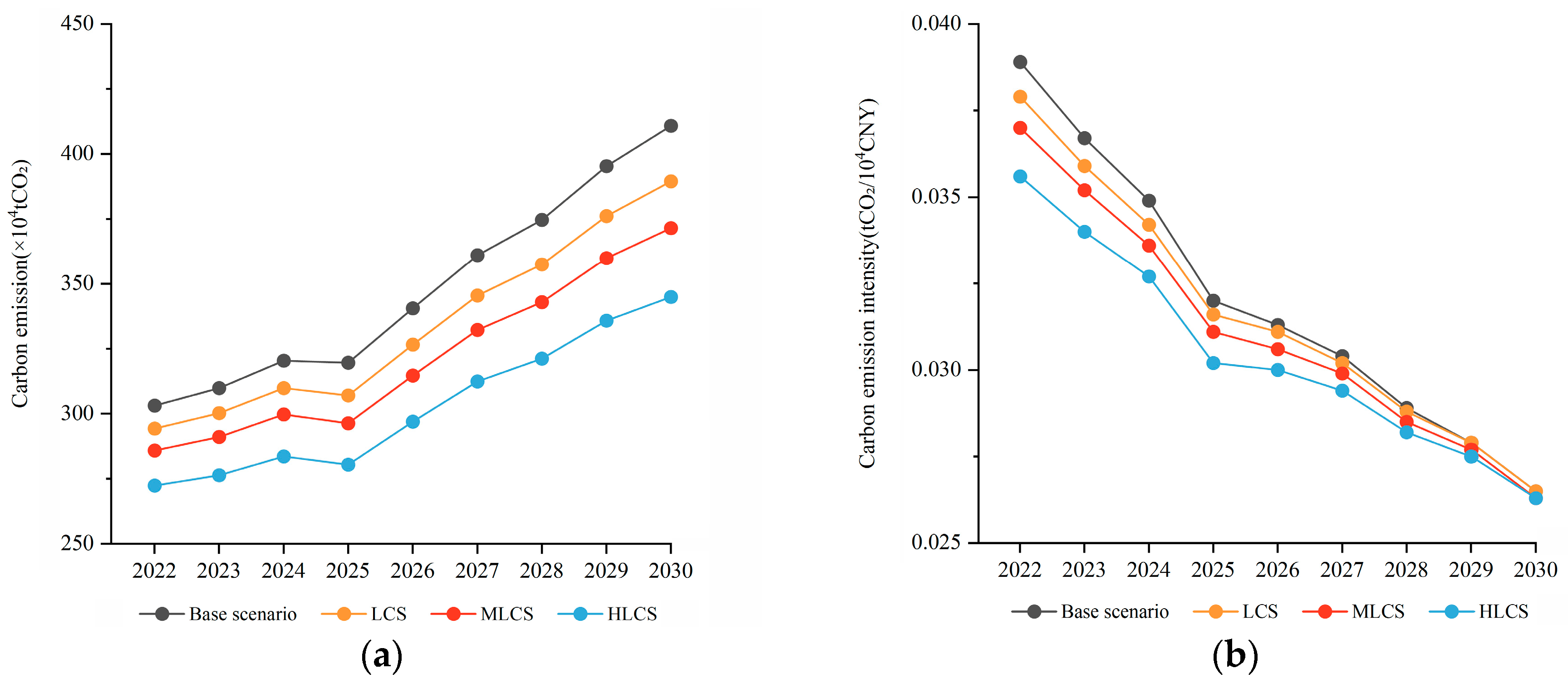
3.3. Simulation of Multi-Factor Carbon Emissions

The residential carbon emission system is characterized by its complexity and dynamic nature, fluctuating with economic and societal growth. As such, regulating a single factor becomes increasingly challenging, necessitating a synergistic approach of multiple policies to support the low-carbon transformation of cities. According to the analysis in Section 3.2 of the study, factors like economic development, urbanization processes, energy consumption levels and structures, low-carbon awareness, and scientific research investments have a significant impact on changes in household carbon emissions in Kunming. After an in-depth examination of these critical factors, the study formulates three scenarios, drawing on references [57,58,59,60] to precisely depict the prevailing conditions in Kunming. As shown in

Table 6. Multi-factor carbon emission scenario modeling options for Kunming, China.

Norm	Base Case	Low-Carbon Scenario (LCS)	Medium Low-Carbon Scenario (MLCS)	High Low-Carbon Scenario (HLCS)
GDP growth rate	Leave the original data unchanged	Reduction of 0.5 percent per year	1% reduction per year	2% reduction per year
Urbanization rate	Leave the original data unchanged	Reduction of 0.5 percent per year	1% reduction per year	2% reduction per year
Energy price	Leave the original data unchanged	1% increase per year	2% increase per year	3% increase per year
Energy consumption structure	Leave the original data unchanged	1.5% increase for natural gas, no change for gas, 1% decrease for LPG, 0.5% decrease for electricity	2% increase for natural gas, no change for gas, 1% decrease for LPG, 1% decrease for electricity	3% increase for natural gas, no change for gas, 1% decrease for LPG, 2% decrease for electricity
Investment in education	Leave the original data unchanged	1% increase per year	2% increase per year	3% increase per year
Investment in scientific research	Leave the original data unchanged	1% increase per year	2% increase per year	3% increase per year

, these scenarios rigorously simulate the influence of several policy interventions on the trend of residential carbon emissions in Kunming, with a specific focus on energy conservation and emission reduction.

The LCS involves a moderate reduction in the rate of growth and urbanization while increasing investment in education and scientific research. The focus is on promoting the development of low-carbon consciousness and technological progress, implementing gradual energy pricing modifications to manage residential energy usage, and increasing the proportion of renewable energy sources. This scenario proposes achieving efficient regulation of carbon emissions from residential areas by implementing a well-coordinated strategy that includes policies, technological advancements, and structural modifications.

The MLCS is an extension of the LCS that implements more rigorous methods to reduce emissions. Additionally, it further slows down urbanization and prioritizes the equitable progress of both economic expansion and carbon emission reduction. This scenario entails increased investment in education and scientific research, modifications to energy prices, and further optimization of the energy consumption structure.

The HLCS is characterized by a modest development rate for Kunming’s economy and urbanization. This entails maintaining lower values for the GDP growth rate and urbanization rate. Building upon the MLCS, the government will enhance funding in the fields of education and scientific innovation, implement higher energy tariffs, and streamline the energy infrastructure. The HLCS embodies a bold strategy for achieving low-carbon development, with a focus on substantial changes in economic and urban growth patterns.

Every scenario is specifically created to examine a plan that combines economic growth with the reduction of residential carbon emissions in a sustainable manner. This provides valuable information on feasible approaches for achieving low-carbon development in Kunming, China.

Figure 9 presents the outcomes of a systematic simulation of various scenarios, projecting residential carbon emissions and carbon emission intensity in Kunming from 2022 to 2030. The base scenario, assuming the continuation of current policies and development trends, forecasts an average annual growth rate of 3.9% in the total residential carbon emissions of Kunming. This translates to an increase of 35.53% from 3,031,200 tons in 2022 to 4,108,200 tons by 2030. In contrast, under the LCS, emissions are projected to be controlled at 3.8951 million tons in 2030, marking a 32.34% increase over 2022 with an average annual growth rate of 3.6%. The LCS also anticipates a cumulative emission reduction of 1.2888 million tons compared to the base scenario.

Similarly, the MLCS is expected to limit emissions to 3.7153 million tons in 2030, a 26.6% increase from 2022, with a modest average annual growth rate of 2.9%. The HLCS shows a more pronounced effect on reducing carbon emissions, with emission reductions ranging from 307,000 tons in 2022 to 659,000 tons by 2030 compared to the base scenario.

The analysis indicates that all scenarios demonstrate a growth in residential carbon emissions, albeit at varying rates. The low-carbon scenarios, particularly the MLCS and HLCS, offer more significant emission reductions compared to the LCS, suggesting the effectiveness of these strategies in curbing the rise of residential carbon emissions in Kunming. The LCS reduces emissions by 143,200 tons annually, while the MLCS and HLCS reduce emissions by 267,900 and 307,000 tons annually, respectively.

4. Discussion

The comprehensive energy conservation and emission reduction program outlined in the Kunming City Plan aims to achieve a GDP exceeding CNY 1 trillion by 2025. Concurrently, it targets a reduction in carbon dioxide emissions and energy consumption per unit of GDP of 18% and 14%, respectively, from the 2020 levels [48]. The simulation results of the three low-carbon development scenarios formulated in this study indicate that each scenario will lead to a decrease in carbon emissions and energy demand, aligning effectively with these planning objectives. Among the scenarios, the MLCS and HLCS exhibit the most substantial impact on emissions reduction. However, the HLCS falls short of meeting the GDP target due to its lower rate of economic growth. Consequently, the MLCS emerges as the most viable option for achieving the dual objectives of the city plan of Kunming—enhancing energy efficiency and reducing carbon emissions while sustaining GDP growth.

The approach to low-carbon urban economic development in China prioritizes maintaining its current level of economic growth and urbanization, which are fundamental and cannot be compromised for carbon emission reduction [61,62]. This necessitates a balance between economic development and environmental conservation, requiring multifaceted strategies, including institutional innovation, technological advancement, and industrial restructuring. A long-term strategy integrating environmental preservation with economic growth is essential. This involves setting phased emission reduction targets across various time frames, creating a systematic roadmap for residential low-carbon development, and implementing these plans at different administrative levels.

Moreover, urbanization should be viewed as an opportunity for transitioning to a low-carbon economy. Balancing urbanization rates with carbon emission increases is crucial. Aggressive energy and environmental policies should be adopted to enhance energy efficiency and structural optimization. Additionally, government incentives such as financial subsidies or tax breaks can motivate businesses to invest in low-carbon technology research and development [63]. This will not only improve the energy efficiency of household appliances but also accelerate the low-carbon development of residential buildings throughout their lifecycle. The government should also lead in enhancing incentive and constraint mechanisms, fostering collaboration among businesses, the public, and other societal actors to promote energy conservation and emission reduction in the residential sector.

Overall, this research offers a valuable exploration of the SD approach for simulating household carbon emissions, considering the geographical characteristics of Kunming. The modeling framework and findings provide a foundational basis for further studies and can be adapted to other cities with similar highland climates, serving as an important reference for policy development and research expansion. However, the models in this study are based on methodological assumptions made to simplify the dynamic complexity associated with characterizing real-world building stocks and energy performance. These assumptions inherently limit the model, warranting caution in its application. Future work could focus on model expansion and refinement to enhance its flexibility and applicability. This might include a thorough evaluation of the effects of potential socio-economic factors on carbon emissions, such as the impact of household income levels on energy usage and transportation choices, the lifestyle and consumption patterns differences between urban and rural dwellers, the level of public awareness and acceptance of environmental conservation and low-carbon lifestyles, as well as the influence of regional industrial structures and energy supply configurations on macroeconomic scales. By quantifying these key factors’ modes of action, a more precise evaluation of the economic and social viability of various emission reduction strategies can be achieved.

5. Conclusions

This study utilized an SD model to simulate urban residential carbon emissions in Kunming, China, for the period 2022–2030 under various scenarios. The key findings from the simulations are summarized as follows:

Growth in Urban Residential Carbon Emissions: The urban residential carbon emissions of Kunming have exhibited a significant increase, with an average annual growth rate of nearly 10% between 2014 and 2021, culminating in an overall rise of 68.7%. This trend is predominantly attributed to the expansion of residential areas and energy consumption driven by urbanization. Despite a temporary decrease in emissions during 2017 and 2018 due to changes in energy use structure, the overall pattern of growth remains consistent.

Projected Increase in Carbon Emissions: Predictions in the study indicate a steep rise in carbon emissions from 2022 to 2030, with an expected peak of 4.108 million tons—almost 2.5 times the 2014 baseline. This underscores the ongoing and future increase in domestic energy consumption and associated carbon emissions.

Influencing Factors and Emission Reduction Strategies: The most significant factors influencing urban residential carbon emissions include economic growth, urbanization, residential energy consumption, and residential investment. Conversely, the key drivers for emission reduction are, in order of effectiveness: enhancing low-carbon awareness, modifying the energy structure, increasing investment in scientific and technological research and development, and expanding green space areas.

Efficacy of Comprehensive vs. Single-Factor Regulation: The study reveals that comprehensive regulation strategies are more effective in reducing emissions compared to single-factor approaches. The MLCS and HLCS demonstrate a higher potential for emission reduction than the standard LCS, particularly the HLCS, which can potentially reduce emissions by up to 20%. However, the HLCS does not align with the 2025 GDP target of CNY 1 trillion. Therefore, it is recommended that, in the short term, the MLCS scenario be targeted to achieve a reduction of about 10% by 2030, balancing economic and environmental pressures. In the medium and long term, investment in science and technology should increase, energy use structure should be optimized, the low-carbon concept of the public should be cultivated, and there should be preparation for achieving a higher level of emission reduction.

This study introduces a pioneering approach to scrutinizing the residential carbon emissions in Kunming, China, a topic that has been relatively underexplored, particularly due to the city’s distinctive highland geography and climate. Through the development of an SD model, this study illuminates the intricate interactions within the complex system of residential carbon emissions in Kunming, thereby offering a more nuanced and accurate depiction of their formation process. To find the best way to reduce emissions while still promoting economic growth and meeting emission reduction goals, the study also started to construct different scenarios that showed how residential carbon emissions might change in the future. These scenarios were used to compare the effects of different emission reduction strategies using numbers. This aids not only in crafting long-term visions but also in devising phased action plans. The methodology and model presented here hold the potential for adaptation across other cities, enabling the development of tailored emission reduction strategies that resonate with local specificities. Moving forward, there is potential to broaden the model to include more emissions sectors, such as industry and transportation, and allow for a comprehensive evaluation of emission reduction initiatives across the entire city.

References

1. IPCC. Climate Change 2023: Synthesis Report. Contribution of Working Groups I. II and III to the Sixth Assessment Report of the Intergovernmental Panel on Climate Change; IPCC: Geneva, Switzerland, 2023; pp. 35–115. [Google Scholar] [CrossRef]
2. Rong, P.; Zhang, Y.; Qin, Y.; Liu, G.; Liu, R. Spatial differentiation of carbon emissions from residential energy consumption: A case study in Kaifeng, China. J. Environ. Manag. 2020, 271, 110895. [Google Scholar] [CrossRef]
3. Chau, C.K.L.; Leung, T.M.; Ng, W.Y. A review on life cycle assessment, life cycle energy assessment and life cycle carbon emissions assessment on buildings. Appl. Energy 2015, 143, 395–413. [Google Scholar] [CrossRef]
4. Geng, J.J.; Wang, J.J.; Huang, J.G.; Zhou, D.; Bai, J.; Wang, J.Y.; Zhang, H.; Duan, H.B.; Zhang, W.B. Quantification of the carbon emission of urban residential buildings: The case of the Greater Bay Area cities in China. Environ. Impact Assess. Rev. 2022, 95, 106775. [Google Scholar] [CrossRef]
5. You, F.H.; Hu, D.; Zhang, H.; Guo, Z.; Zhao, Y.; Wang, B.; Yuan, Y. Carbon emissions in the life cycle of urban building system in China—A case study of residential buildings. Ecol. Complex. 2011, 8, 201–212. [Google Scholar] [CrossRef]
6. Burleyson, C.D.; Iyer, G.; Hejazi, M.; Kim, S.; Kyle, P.; Rice, J.S.; Smith, A.D.; Taylor, Z.T.; Voisin, N.; Xie, Y.L. Future western US building electricity consumption in response to climate and population drivers: A comparative study of the impact of model structure. Energy 2020, 208, 118312. [Google Scholar] [CrossRef]
7. Wang, Q.; Lin, J.; Zhou, K.; Fan, J.; Kwan, M.P. Does urbanization lead to less residential energy consumption? A comparative study of 136 countries. Energy 2020, 202, 117765. [Google Scholar] [CrossRef]
8. Huo, T.F.; Li, X.H.; Cai, W.G.; Zuo, J.; Jia, F.Y.; Wei, H.F. Exploring the impact of urbanization on urban building carbon emissions in China: Evidence from a provincial panel data model. Sustain. Cities Soc. 2020, 56, 102068. [Google Scholar] [CrossRef]
9. Gan, L.; Liu, Y.; Shi, Q.; Cai, W.; Ren, H. Regional inequality in the carbon emission intensity of public buildings in China. Build. Environ. 2022, 225, 109657. [Google Scholar] [CrossRef]
10. Wu, L.F.; Huang, G.M.; Fan, J.L.; Zhang, F.C.; Wang, X.K.; Zeng, W.Z. Potential of kernel-based nonlinear extension of Arps decline model and gradient boosting with categorical features support for predicting daily global solar radiation in humid regions. Energy Convers. Manag. 2019, 183, 280–295. [Google Scholar] [CrossRef]
11. Trotta, G. Factors affecting energy-saving behaviours and energy efficiency investments in British households. Energy Policy 2018, 114, 529–539. [Google Scholar] [CrossRef]
12. Wan, C.; Shen, G.Q.; Choi, S. The moderating effect of subjective norm in predicting intention to use urban green spaces: A study of Hong Kong. Sustain. Cities Soc. 2018, 37, 288–297. [Google Scholar] [CrossRef]
13. Shi, H.X.; Wang, S.Y.; Zhao, D.T. Exploring urban resident’s vehicular PM2.5 reduction behavior intention: An application of the extended theory of planned behavior. J. Clean. Prod. 2017, 147, 603–613. [Google Scholar] [CrossRef]
14. Liu, X.; Wang, Q.C.; Wei, H.H.; Chi, H.L.; Ma, Y.T.; Jian, I.Y. Psychological and Demographic Factors Affecting Household Energy-Saving Intentions: A TPB-Based Study in Northwest China. Sustainability 2020, 12, 836. [Google Scholar] [CrossRef]
15. Fan, J.B.; Ran, A.B.; Li, X.M. A Study on the Factors Affecting China’s Direct Household Carbon Emission and Comparison of Regional Differences. Sustainability 2019, 11, 4919. [Google Scholar] [CrossRef]
16. Li, J.B.; Huang, X.J.; Yang, H.; Chuai, X.W.; Li, Y.; Qu, J.S.; Zhang, Z.Q. Situation and determinants of household carbon emissions in Northwest China. Habitat Int. 2016, 51, 178–187. [Google Scholar] [CrossRef]
17. Fremstad, A.; Underwood, A.; Zahran, S. The Environmental Impact of Sharing: Household and Urban Economies in CO2 Emissions. Ecol. Econ. 2018, 145, 137–147. [Google Scholar] [CrossRef]
18. Paone, A.; Bacher, J.P. The Impact of Building Occupant Behavior on Energy Efficiency and Methods to Influence It: A Review of the State of the Art. Energies 2018, 11, 953. [Google Scholar] [CrossRef]
19. Hu, Z.; He, J.; Wang, Y. Factor analysis and enlightenment of household carbon emissions in Japan based on IPAT-LMDI extension model. Resour. Sci. 2018, 40, 1831–1842. [Google Scholar]
20. Li, Z.; Liu, Y.Z.; Zhang, Z. Carbon Emission Characteristics and Reduction Pathways of Urban Household in China. Front. Environ. Sci. 2022, 10, 896765. [Google Scholar] [CrossRef]
21. Jin, J.; Wang, Y.C.; Zheng, X.Y. District heating versus self-heating: Estimation of energy efficiency gap using regression discontinuity design. China Econ. Q. Int. 2021, 1, 208–220. [Google Scholar] [CrossRef]
22. Payne, S.; Barker, A. Carbon regulation and pathways for institutional transition in market-led housing systems: A case study of English housebuilders and zero carbon housing policy. Environ. Plan. E-Nat. Space 2018, 1, 470–493. [Google Scholar] [CrossRef]
23. Zhang, X.F.; Fan, D.C. The Spatial-Temporal Evolution of China’s Carbon Emission Intensity and the Analysis of Regional Emission Reduction Potential under the Carbon Emissions Trading Mechanism. Sustainability 2022, 14, 7442. [Google Scholar] [CrossRef]
24. Li, H.; Cao, L.; Chen, Y.B.; Qiu, H.Y.; Huang, X.; Guo, W.Q.; Wang, S.T.; Sheng, W.G.; Zhou, Y.L.; Xu, Q. Emergy analysis-based study of the sustainable development of Kunming’s urban eco-economic system. Int. J. Urban Sci. 2023, 27, 322–343. [Google Scholar] [CrossRef]
25. Shao, P.; Xin, J.Y.; Zhang, X.L.; Gong, C.S.; Ma, Y.J.; Wang, Y.S.; Wang, S.G.; Hu, B.; Ren, X.B.; Wang, B.Y. Aerosol optical properties and their impacts on the co-occurrence of surface ozone and particulate matter in Kunming City, on the Yunnan-Guizhou Plateau of China. Atmos. Res. 2022, 266, 105963. [Google Scholar] [CrossRef]
26. Gao, Y.; Pitts, A.; Amsterdam Univ, P. The Ancient Southern Silk Road and the Contemporary One Belt and One Road in Southwest China Case study of Kunming City in Yunnan Province. In Proceedings of the 12th International Convention of Asia Scholars (ICAS), Electr Network, 24–28 August 2021; pp. 177–182. [Google Scholar]
27. Liu, Z.; Sun, T.; Yu, Y.; Ke, P.; Deng, Z.; Lu, C.; Huo, D.; Ding, X. Near-Real-Time Carbon Emission Accounting Technology Toward Carbon Neutrality. Engineering 2022, 14, 44–51. [Google Scholar] [CrossRef]
28. Wen, Z.; Yang, Z.; Xing, Q. A comprehensive evaluation of regional carbon emission based on the composite model in China: A case study of Huaibei city (China). Sci. Rep. 2023, 13, 15387. [Google Scholar] [CrossRef] [PubMed]
29. Xiong, P.; Wu, X.; Ye, J. Building a novel multivariate nonlinear MGM(1,m,N|γ) model to forecast carbon emissions. Environ. Dev. Sustain. 2023, 25, 9647–9671. [Google Scholar] [CrossRef]
30. Oh, J.; Hong, T.; Kim, H.; An, J.; Jeong, K.; Koo, C. Advanced Strategies for Net-Zero Energy Building: Focused on the Early Phase and Usage Phase of a Building’s Life Cycle. Sustainability 2017, 9, 2272. [Google Scholar] [CrossRef]
31. Schmidt, M.; Crawford, R.H. A framework for the integrated optimisation of the life cycle greenhouse gas emissions and cost of buildings. Energy Build. 2018, 171, 155–167. [Google Scholar] [CrossRef]
32. Zhong, X.; Li, X.; Li, Y. Urban Expansion and Carbon Emission Logistic Curve Hypothesis and Its Verification: A Case Study of Jiangsu Province. Land 2022, 11, 1066. [Google Scholar] [CrossRef]
33. Cheng, S.; Zhou, X.; Zhou, H. Study on Carbon Emission Measurement in Building Materialization Stage. Sustainability 2023, 15, 5717. [Google Scholar] [CrossRef]
34. People’s Government of Kunming. Kunming Statistical Yearbook. Available online: https://www.km.gov.cn/zfxxgk/fdzdgknr/tjxx/jjyxqk/tjnj/ (accessed on 18 January 2024).
35. National Bureau of Statistics of China. Kunming Statistical Yearbook (2014–2021). Available online: https://www.stats.gov.cn/sj/ndsj/2022/indexeh.htm (accessed on 20 January 2024).
36. National Development and Reform Commission of China. Technology Policy for Upgrading Coal Power Units for Energy Conservation and Emission Reduction. Available online: https://www.cmenhu.cn/13448.html (accessed on 20 January 2024).
37. Zhou, G.H.; Chung, W.; Zhang, Y.X. Carbon dioxide emissions and energy efficiency analysis of China’s regional thermal electricity generation. J. Clean. Prod. 2014, 83, 173–184. [Google Scholar] [CrossRef]
38. Huang, Y.S.; Shen, L.; Liu, H. Grey relational analysis, principal component analysis and forecasting of carbon emissions based on long short-term memory in China. J. Clean. Prod. 2019, 209, 415–423. [Google Scholar] [CrossRef]
39. Kim, G.; Jong, Y.; Liu, S.F. Generalized Hybrid Grey Relation Method for Multiple Attribute Mixed Type Decision Making. J. Grey Syst. 2014, 26, 142–153. [Google Scholar]
40. Sun, Y.M.; Liu, S.X.; Li, L. Grey Correlation Analysis of Transportation Carbon Emissions under the Background of Carbon Peak and Carbon Neutrality. Energies 2022, 15, 3064. [Google Scholar] [CrossRef]
41. Lv, T.G.; Hu, H.; Zhang, X.M.; Sun, L.; Li, Z.L.; Chen, Y.J.; Fu, S.F. Driving mechanism of the allometric relationship between economic development and carbon emissions in the Yangtze River Delta urban agglomeration, China. Environ. Dev. Sustain. 2023. [Google Scholar] [CrossRef]
42. Forrester, J.W. System dynamics—The next fifty years. Syst. Dyn. Rev. 2007, 23, 359–370. [Google Scholar] [CrossRef]
43. Zhan, J.Y.; Wang, C.; Wang, H.H.; Zhang, F.; Li, Z.H. Pathways to achieve carbon emission peak and carbon neutrality by 2060: A case study in the Beijing-Tianjin-Hebei region, China. Renew. Sustain. Energy Rev. 2024, 189, 113955. [Google Scholar] [CrossRef]
44. Huo, T.F.; Ma, Y.L.; Xu, L.B.; Feng, W.; Cai, W.G. Carbon emissions in China’s urban residential building sector through 2060: A dynamic scenario simulation. Energy 2022, 254, 124395. [Google Scholar] [CrossRef]
45. Huo, T.F.; Xu, L.B.; Feng, W.; Cai, W.G.; Liu, B.S. Dynamic scenario simulations of carbon emission peak in China’s city-scale urban residential building sector through 2050. Energy Policy 2021, 159, 112612. [Google Scholar] [CrossRef]
46. Murray, P.; Marquant, J.; Niffeler, M.; Mavromatidis, G.; Orehounig, K. Optimal transformation strategies for buildings, neighbourhoods and districts to reach CO2 emission reduction targets. Energy Build. 2020, 207, 109569. [Google Scholar] [CrossRef]
47. Liu, L.Y.; Tang, Y.L.; Chen, Y.Y.; Zhou, X.; Bedra, K.B. Urban Sprawl and Carbon Emissions Effects in City Areas Based on System Dynamics: A Case Study of Changsha City. Appl. Sci. 2022, 12, 3244. [Google Scholar] [CrossRef]
48. Kunming People’s Government. The 14th Five-Year Plan for the National economic and Social Development of Kunming City and the Outline of the Long-Term Goals for 2035. Available online: https://www.km.gov.cn/c/2021-04-06/3890927.shtml (accessed on 20 January 2024).
49. Chicco, D.; Warrens, M.J.; Jurman, G. The coefficient of determination R-squared is more informative than SMAPE, MAE, MAPE, MSE and RMSE in regression analysis evaluation. Peerj Comput. Sci. 2021, 7, e623. [Google Scholar] [CrossRef] [PubMed]
50. Uyanto, S.S. Power comparisons of five most commonly used autocorrelation tests. Pak. J. Stat. Oper. Res. 2020, 16, 119–130. [Google Scholar] [CrossRef]
51. Shrestha, N. Detecting Multicollinearity in Regression Analysis. Am. J. Appl. Math. Stat. 2020, 8, 39–42. [Google Scholar] [CrossRef]
52. Liu, J.K.; Liu, Y.D.; Wang, X.T. An environmental assessment model of construction and demolition waste based on system dynamics: A case study in Guangzhou. Environ. Sci. Pollut. Res. 2020, 27, 37237–37259. [Google Scholar] [CrossRef] [PubMed]
53. Ning, X.; He, Y.; Zhang, J.; Wu, C.; Zhang, Y. Analysis of Carbon Emission Projections and Reduction Potential of Resource-Dependent Urban Agglomerations from the Perspective of Multiple Scenarios-A Case Study of Hu-Bao-O-Yu Urban Agglomeration. Int. J. Environ. Res. Public Health 2023, 20, 4250. [Google Scholar] [CrossRef] [PubMed]
54. Tian, X.; Geng, Y.; Dong, H.; Dong, L.; Fujita, T.; Wang, Y.; Zhao, H.; Wu, R.; Liu, Z.; Sun, L. Regional household carbon footprint in China: A case of Liaoning province. J. Clean. Prod. 2016, 114, 401–411. [Google Scholar] [CrossRef]
55. Oda, T.; Feng, L.; Palmer, P.; Baker, D.F.; Ott, L.E. Assumptions about prior fossil fuel inventories impact our ability to estimate posterior net CO2 fluxes that are needed for verifying national inventories. Environ. Res. Lett. 2023, 18, 124030. [Google Scholar] [CrossRef]
56. Schernikau, L.; Smith, W.H. Climate impacts of fossil fuels in today’s electricity systems. J. S. Afr. Inst. Min. Metall. 2022, 122, 133–145. [Google Scholar] [CrossRef]
57. Zheng, X.Q.; Wang, J.Y.; Chen, Y.; Tian, C.; Li, X.M. Potential pathways to reach energy-related CO2 emission peak in China: Analysis of different scenarios. Environ. Sci. Pollut. Res. 2023, 30, 66328–66345. [Google Scholar] [CrossRef] [PubMed]
58. Sun, X.M.; Zhang, H.T.; Wang, X.Y.; Qiao, Z.K.; Li, J.S. Towards Sustainable Development: A Study of Cross-Regional Collaborative Carbon Emission Reduction in China. Sustainability 2022, 14, 9624. [Google Scholar] [CrossRef]
59. Ge, X.X.; Qi, W. Analysis of CO2 Emission Drives Based on Energy Consumption and Prediction of Low Carbon Scenarios: A Case Study of Hebei Province. Pol. J. Environ. Stud. 2020, 29, 2185–2197. [Google Scholar] [CrossRef]
60. Ayuketah, Y.; Gyamfi, S.; Diawuo, F.A.; Dagoumas, A.S. Assessment of low-carbon energy transitions policies for the energy demand sector of Cameroon. Energy Sustain. Dev. 2023, 72, 252–264. [Google Scholar] [CrossRef]
61. Wang, J.Y.; He, D.Q. Sustainable urban development in China: Challenges and achievements. Mitig. Adapt. Strateg. Glob. Chang. 2015, 20, 665–682. [Google Scholar] [CrossRef]
62. Wu, H.L.; Wang, L.; Peng, D.X.; Liu, B.J. Input-output efficiency model of urban green-energy development from the perspective of a low-carbon economy. Clean Energy 2022, 6, 905–916. [Google Scholar] [CrossRef]
63. Liu, Y.; Cui, J.F.; Jiang, H.; Yan, H. Do county financial marketization reforms promote food total factor productivity growth?: A mechanistic analysis of the factors quality of land, labor, and capital. Front. Sustain. Food Syst. 2023, 7, 1263328. [Google Scholar] [CrossRef]
Figure 1. Research framework.
Buildings 14 00982 g001
Figure 2. Location of the study area.
Buildings 14 00982 g002
Figure 3. Urban residential carbon emissions and per capita carbon emissions from different energy sources in Kunming, China, spanning the years 2014 to 2021.
Buildings 14 00982 g003
Figure 4. Key influencing factors of carbon emissions from residential buildings in Kunming, China. (a) The energy consumption expenditure of residents; (b) energy prices; (c) heating degree days.
Buildings 14 00982 g004aBuildings 14 00982 g004b
Figure 5. The framework of the system dynamics (SD) model.
Buildings 14 00982 g005
Figure 6. Causal loop diagrams of (a) economic subsystems, (b) social subsystems, (c) energy subsystems, and (d) environmental subsystems. +: incremental effect, −: reducing effect.
Buildings 14 00982 g006
Figure 7. Stock–flow diagram.
Buildings 14 00982 g007
Figure 8. Carbon emission and carbon emission intensity of urban housing in Kunming, China, 2014–2021.
Buildings 14 00982 g008
Figure 9. Trend chart of (a) carbon emission and (b) carbon emission intensity changes in different scenarios for Kunming, China.
Buildings 14 00982 g009