Abstract
This paper investigates a method for improving the selection of seismic motions for designing earthquake-resistant underground structures. It is found that PGV alone is unreliable as a predictor of structural damage with increasing earthquake intensity. Therefore, based on characterizing seismic intensity by using PGV, another parameter, referred to here as “the severest parameter”, is introduced to distinguish potential damage capacity for different seismic motions. A numerical model of a soil–underground structure system was established using the finite element software OpenSees. A total of 120 real ground motions were selected for the model, considering the influences of eight different site groups on the underground station and the rupture distances of the input seismic motions. The results show that as seismic intensity increases, substantial variability in the response of underground structures emerges under the same amplitude of PGV, diminishing the effectiveness of the relationship between PGV and structural damage. When assessing the potential damage capacity of seismic motions with similar or close amplitudes of PGV, VSI is an appropriate severest parameter for Class III sites and ASI is suitable for Class II sites. When the correlation coefficient between the severest parameter and the structural response is greater than 0.8, it can be used to reliably assess seismic damage capacity based on the size of the severest parameter.
1. Introduction
Selecting rational ground motion records is the most important step prior to the seismic analysis and design of underground structures. Different input ground motion records may lead to significantly different responses in structures. Therefore, Drenick [1] introduced the “critical excitation method” in order to determine the excitation that maximizes the demands on a given system under specific constraints. Scholars have applied this concept to various research subjects, such as linear structures [2], nonproportionally damped structural systems [3], and tuned mass dampers [4].
On the basis of the “critical excitation method”, Xie and Zhai [5] introduced the concept of the “severest seismic motion”, which aims to identify seismic motions that lead the structure to sustain the most severe damage state under the premise of meeting fortification intensity and site requirements for the structure. The key to this concept lies in finding the seismic intensity indicator that best reflects the potential damage capacity of seismic motion.
Scholars have previously constructed the multivariate distribution of any set of ground-motion intensity measures [6] or developed parametric equations [7] for the selection of ground motions. Li et al. [8] proposed a methodology for selecting the severest ground motions for practical dynamic analyses of nuclear power plant (NPP) systems. A series of correlation analyses were carried out to select the relevant intensity measures that best characterize the structural demand parameters, and consequently the damage potential, of ground motions on NPP structures. Zhai et al. [9] selected those real (or recorded) ground motions capable of exposing low- and mid-rise reinforced concrete frame structures to an extreme limit state. By performing correlation analyses, two optimal intensity measures were selected to represent the ground motion damage potential. The concept of the severest seismic motion has been applied to earth dams as well [10,11]. Chen et al. [12] proposed a ranking method based on a composite intensity indicator for the severest input ground motion for underground structures. The results show that the proposed composite ground motion intensity indicators have a higher correlation with the seismic dynamic responses than a single indicator with respect to effectiveness, practicability, and proficiency.
Several scholars have stated that “efficiency” and “sufficiency” are two evaluation dimensions of seismic intensity indicators, and have proposed seismic intensity parameters that are suitable for different structural forms and seismic characteristics. In research on underground structures, the Peak Ground Acceleration (PGA) is a widely used seismic intensity indicator in structural seismic analysis and design [13,14,15,16,17,18,19]. With the rapid development of seismic research on underground structures, scholars have found that the Peak Ground Velocity (PGV) is suitable for seismic damage assessment of underground structures. Tsinidis et al. [20] investigated the efficiency and sufficiency of various seismic intensity measures for the structural assessment of buried steel natural gas (NG) pipelines and found that the PGV is the optimal IM. In the context of underground tunnels, Corigliano et al. [21] found a better correlation between seismic damage in underground tunnels and PGV compared to PGA. When studying the optimal seismic intensity indicator for tunnels at different depths, Huang et al. [22] evaluated the effectiveness by using dispersion under double logarithmic linear regression, and found that PGV consistently performed the best. Liu et al. [23] discovered that PGV had a higher regression fitting accuracy with the inter-story drift angle of an underground station, with a smaller standard deviation than PGA. Zhang et al. [24] investigated the optimal seismic intensity indicators for a three-span three-story station at different burial depths, and indicated that PGV was the most suitable indicator. Therefore, compared to PGA, PGV is more suitable as a seismic intensity indicator for assessing the seismic performance of underground structures. In predicting the damage potential of seismic motions, PGV is an important indicator that must be taken into account.
However, it has been found that a single parameter cannot describe all seismic characteristics. Only one parameter, whether PGA, PGV, or other parameters, cannot comprehensively and accurately evaluate the correlation between seismic intensity and structural damage. Accordingly, previous scholars have introduced optimization algorithms to construct mixed seismic parameters with the highest correlation with structural damage [25,26,27]. These optimization algorithms are computationally complex. The correlation between the constructed mixed seismic parameters and structural damage is greatly affected by the optimization algorithm used, making them inconvenient to apply in seismic design. Therefore, scholars have combined multiple seismic intensity parameters [28,29], which is more convenient than using optimization algorithms. The research design of this paper was derived from this concept.
The main objective of this paper is to propose a method for selecting the seismic motion with the greatest damage potential based on the “severest parameter” for underground stations. In the seismic design of structures, it is necessary to input the near-field and far-field seismic motions separately and to consider the stiffness of the site. Therefore, different types of rupture distances of seismic motions and different site stiffness values were considered. The selection method proposed in this paper requires two steps. First, the PGV of the input seismic motions is normalized to a consistent value and its deficiency in predicting seismic damage potential is verified. Second, based on the same PGV amplitude, another parameter, referred to here as the “severest parameter”, is selected through a correlation analysis with the structural seismic responses. Finally, the applicability of this selection method is verified through the color mapping method, which can provide visual effects to show the strength and weakness of seismic potential damage capacity. The selection method provided in this paper improves upon the limitations of PGV alone in estimating seismic damage potential. In the seismic design of underground stations, when the input seismic motions have similar or identical amplitudes to that of PGV, their damage potential can be evaluated based on the research results of this paper.
2. Numerical Model of Soil–Underground Station System
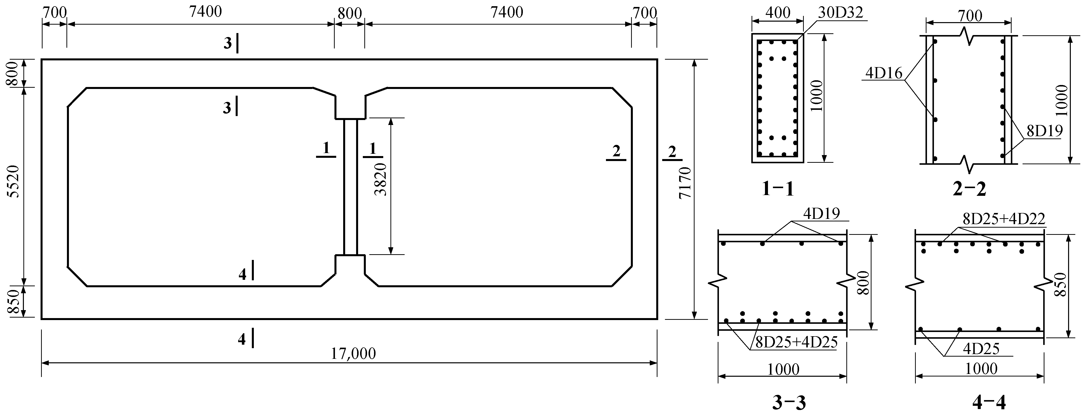
This paper takes the Daikai station, damaged in the 1995 Kobe Earthquake, as its research subject. According to the investigation [30], the station had a cross-sectional dimension of 17 m × 7.17 m, a top slab thickness of 0.8 m, a bottom slab thickness of 0.85 m, and a side wall thickness of 0.7 m. The cross-sectional dimensions of the central columns were 0.4 m × 1.0 m, with a longitudinal spacing of 3.5 m and an effective height of 3.82 m. The main section dimensions and reinforcement details are shown in Figure 1. The concrete strength of the central columns was 23.52 MPa, while the concrete strength of the other parts of the structure was 20.58 MPa. In this paper, the station structure is considered to be buried to a depth of 4 m.

Figure 1.
Section dimension and reinforcement details of Daikai Station (Unit: mm).
The Daikai station was established using OpenSees v3.2.2 finite element software. The thickness of the model was set to 3.5 m based on longitudinal spacing of the central columns. The concrete was modeled with the Kent–Scott–Park constitutive model (Concrete01 Material) without taking tensile strength into account. The steel reinforcement was modeled using a uniaxial bilinear constitutive model (Steel01 Material). Specific material parameters can be found in Table 1.

Table 1.
Material properties of the concrete and steel reinforcement.
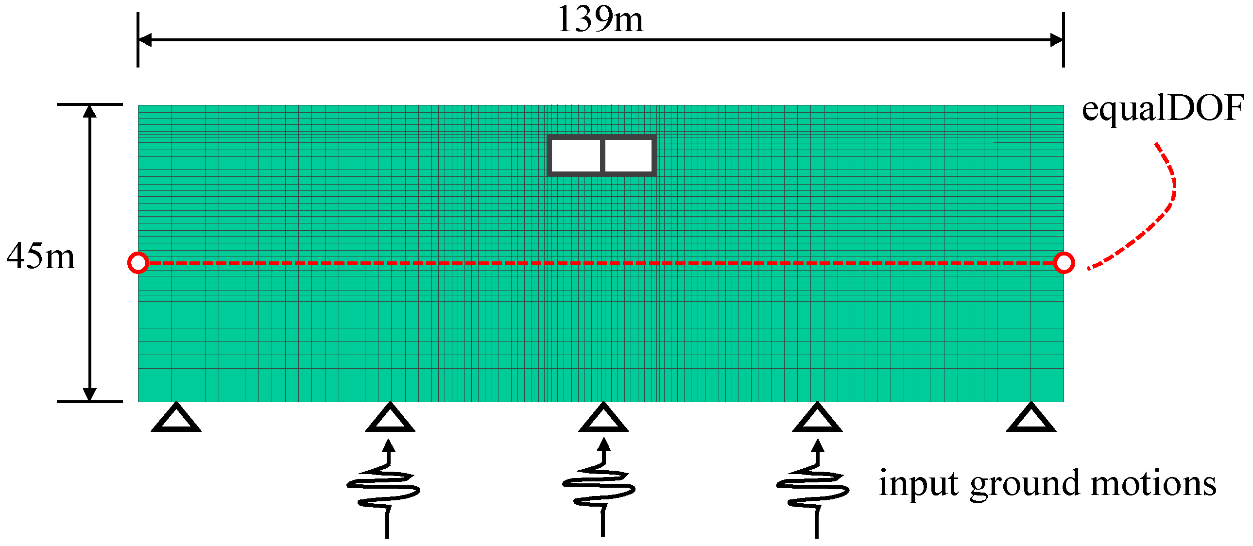
The finite element model of the soil–underground station system is shown in Figure 2. The dimension of the soil domain is 139 m × 45 m × 3.5 m (wide × height × length). According to the Code for the Seismic Design of Buildings (GB50011, 2010), the width of the soil on each side surrounding the structure should be at least three times larger than the width of the structure in order to avoid ground motion reflection, while the depth of the model should be more than three times the height of the station.

Figure 2.
Finite element model of soil–underground station system.
For the boundary conditions of the 2D model, the semi-infinite soil domain was truncated at a distance of 61 m from the structure (more than three times the width of the structure), which is sufficiently far from the underground structure to eliminate the influence of the boundary effects on the seismic response of the underground structure. The bottom boundary of the 2D model was truncated at a depth of 45 m. The longitudinal thickness of the soil matched the station model at 3.5 m. The burial depth from the top of the reinforced concrete roof of the station to the ground surface was about 4 m.
The horizontal and vertical displacements were fixed at the bottom surface, while the ground surface of the structure was free. Using the equalDOF command, horizontal kinematic constraints were introduced to the nodes on two side boundaries in order to ensure the same horizontal movement of the two nodes at the same burial depth, which effectively simulates the shear deformations of the soil layers under upward propagation of in-plane waves [31].
Four-node quad elements were employed in the numerical model for the surrounding soil. The material of the soil domain was PressureIndependMultiYield (PIMY) with yield surfaces of the Von Mises type.
As the overall depth of the soil layers above the engineering bedrock were smaller than 50 m, according to the Chinese code for seismic design of urban rail transit structures the equivalent shear wave velocities of Classes II and III range from 150 m/s to 500 m/s and from 90 m/s to 150 m/s.
By distinguishing the shear wave velocities, this paper designed five scenarios for Class II sites and three scenarios for Class III sites. Incorporating the recommended values for the PressureIndependMultiYield constitutive model from the OpenSees user manual, the physical parameters of the soil for the two site categories are presented in Table 2, including the density ρ, initial shear modulus G, initial shear velocity Vs20, Poisson’s ratio μ, cohesion c, and friction angle φ.
Table 2.
Geotechnical properties of soils in different site categories.
3. Seismic Waves and Selection of the Severest Parameter
3.1. Seismic Wave Selection
This paper investigated the effects of rupture distance (R) and site class on underground stations by selecting seismic motions from the PEER Ground Motions Database with moment magnitudes exceeding 6.0. For site classification, shear wave velocity was used. Class II sites have a velocity of 260 m/s to 510 m/s, while Class III sites range from 150 m/s to 260 m/s.
In seismic engineering design, it is necessary to input the near-field and far-field ground motions separately for seismic analysis. Scholars have classified near-fault records when R is less than or equal to 20 km [32,33] and far-fault records when R is 20 km to 60 km [34]. In order to enhance the differentiation between near-field and far-field earthquakes, in this paper we have relaxed the classification based on rupture distance; near-field ground motions were defined with R ≤ 20 km and far-field ground motions were defined with R ≥ 80 km. Between near-field and far-field earthquakes, this paper defines ordinary ground motions with 30 km ≤ R ≤ 70 km as a transitional zone. Therefore, based on two sites and three types of rupture distances, the selected seismic motions are divided into six groups. Considering that the literature [35] indicates that 20 input seismic motions in the IDA method is sufficient to capture the uncertainties in seismic records, 20 seismic motions were selected for each group, totaling 120 seismic motions in all.
3.2. The Severest Parameters
To better characterize seismic intensity based on PGV, another parameter, referred to here as “the severest parameter”, was introduced to distinguish the potential damage capacity for different seismic motions. Specifically, the severest parameter refers to the seismic characteristic parameter that shows the strongest correlation with structural response under the seismic motions with the same PGV. The parameters preselected in this paper as the severest parameters can be categorized into four classes: acceleration-related parameters, velocity-related parameters, displacement-related parameters, and hybrid parameters [36,37].
Most of the formulations are similar, with the following differences: ① differing by only one exponent in the expression; ② differing by only one constant in the expression; and ③ being a linear combination of the other parameters in logarithmic coordinates. Therefore, after the selection process, in this paper we have chosen nine highly representative least favorable indicators for subsequent analysis; the specific expressions of the indicators can be found in Table 3.
Table 3.
The optional severest parameters.
In this table, ttot represents the total duration of the seismic motion; a(t), v(t), and d(t) represent the acceleration, velocity, and displacement time histories, respectively; Sa, Sv, and Sd represent the spectral acceleration, spectral velocity, and spectral displacement, respectively; and t95 and t5 respectively represent the times corresponding to 95% and 5% of the Arias intensity IA.
In addition, PGA and PGD reflect the amplitude of seismic motion; asq, vsq, and dsq reflect the input energy of seismic motion; ASI, VSI, and DSI reflect the spectral intensity within the periodic range of the seismic motion; and td represents the significant duration of the seismic motion, reflecting the characteristics of strong motion duration.
In order to evaluate the applicability of the parameters, correlation coefficients were calculated to show the relationship between structural response and the severest parameter, with the calculation formula shown in Equation (1):
In the above formula, x and y respectively represent the structural response and the severest parameter, Cov(x,y) is the covariance between x and y, and Var[x] and Var[y] are the variances of x and y, respectively. It is generally believed that an absolute value of ρ between 0.6 and 0.8 represents a high correlation, while a value between 0.8 and 1.0 represents a very strong correlation.
4. Result Analysis
4.1. Distribution Pattern of Structural Response
In this paper, we used the maximum inter-story drift angle of the underground station as the structural damage indicator and performed IDA analysis after scaling the PGV of the seismic motions to 10 cm/s, 20 cm/s, 40 cm/s, 80 cm/s, and 120 cm/s. The Class II site condition with shear wave velocity of 280 m/s was taken as an example.
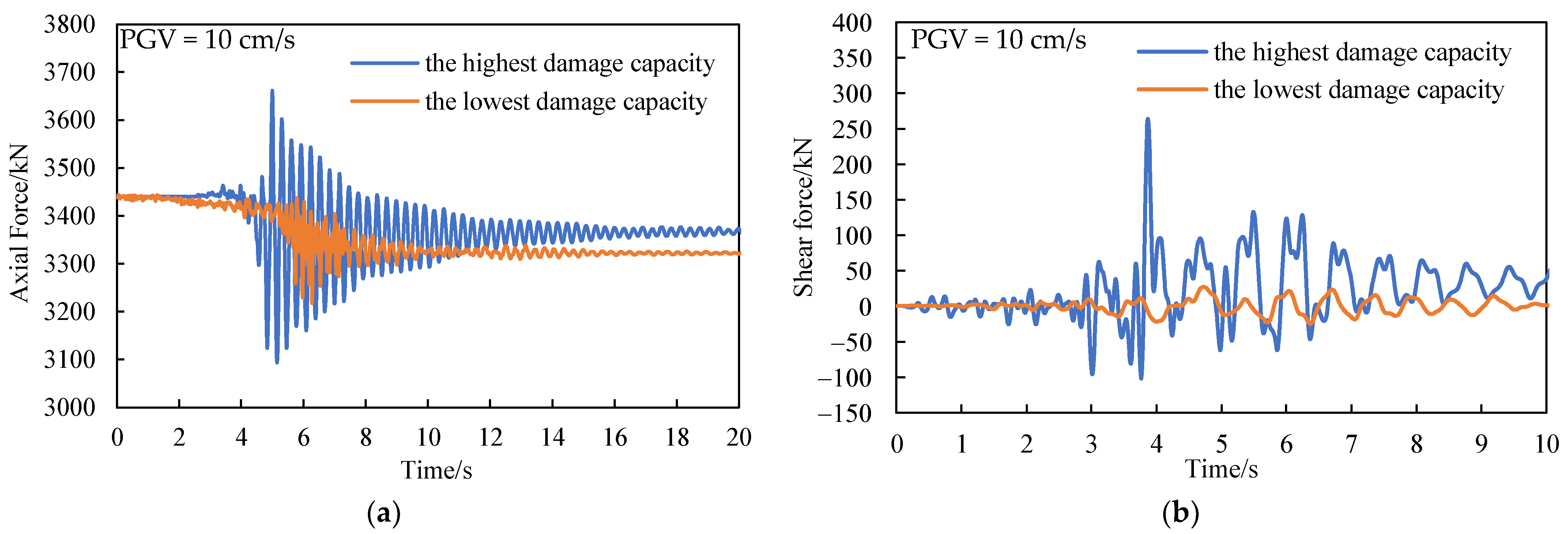
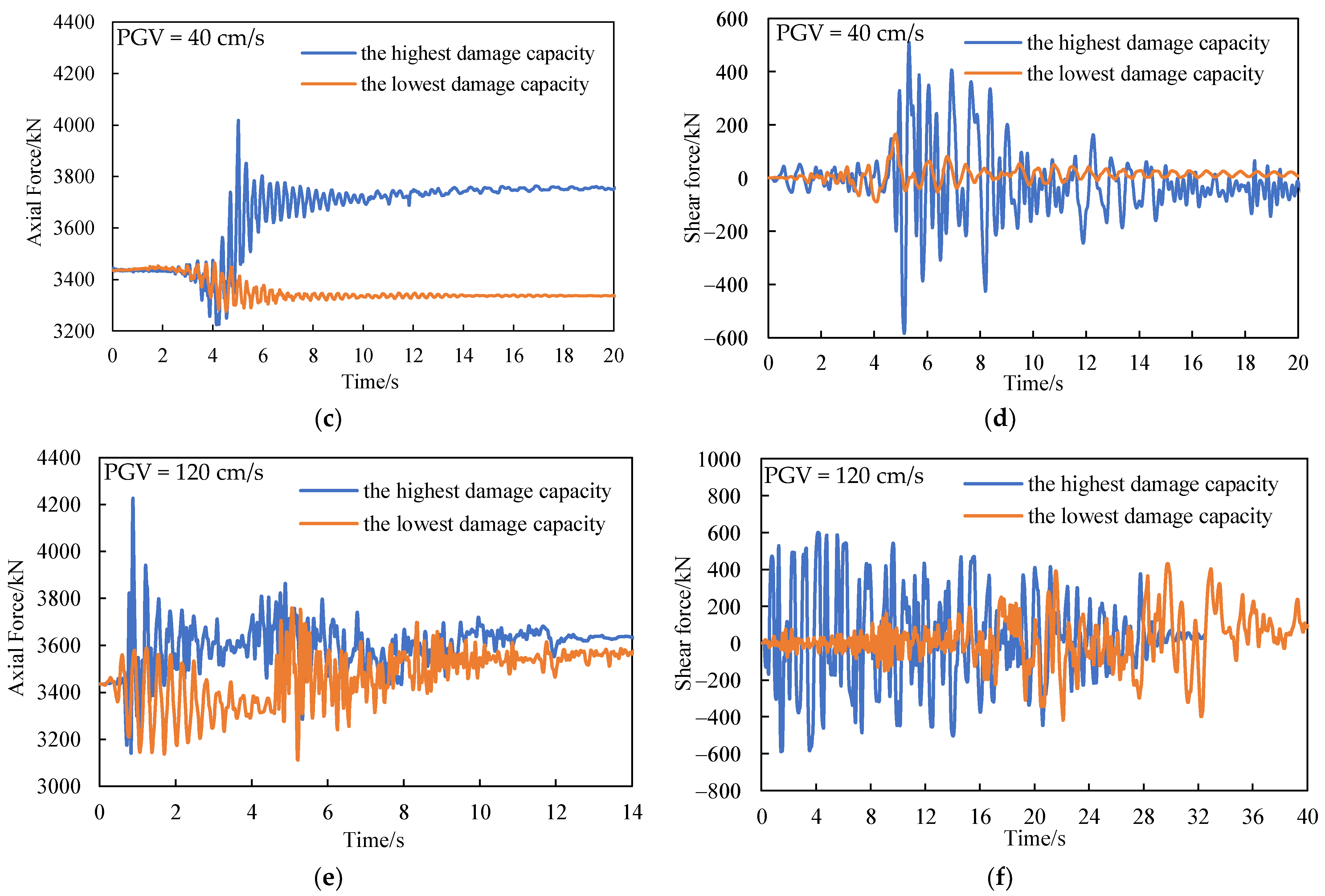
The axial force time history curves were extracted when the peak axial forces in the central column reached their maximum and minimum values under seismic actions with the same PGV amplitude. The shear force time history curves for the central column were extracted using the same method. The results are shown in Figure 3. In order to create a sharp contrast in the figures, three conditions were selected while PGV was 10 cm/s, 40 cm/s, and 120 cm/s.
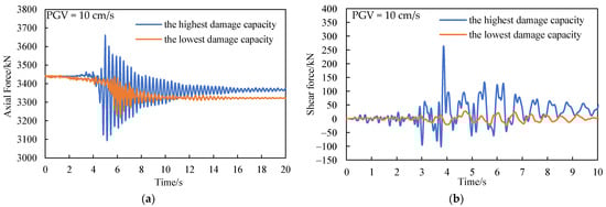
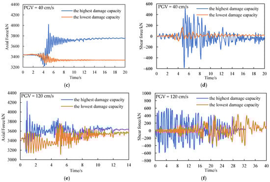
Figure 3.
Time history curve of axial force and shear force: (a) axial force time history curve, PGV = 10 cm/s; (b) shear force time history curve, PGV = 10 cm/s; (c) axial force time history curve, PGV = 40 cm/s; (d) shear force time history curve, PGV = 40 cm/s; (f) axial force time history curve, PGV = 120 cm/s; (e) shear force time history curve, PGV = 120 cm/s.
The relationship between seismic intensity and structural forces was then investigated. The central column’s axial force under gravity load is 3435.53 kN. When subjected to seismic actions with PGV of 10 cm/s, the axial force reaches a maximum of 3661.29 kN and a minimum of 3446.75 kN. As the PGV increases to 40 cm/s and 120 cm/s, the range of peak axial forces increases as well. Similarly, the peak shear force of the central column displays a rising trend with higher PGV.
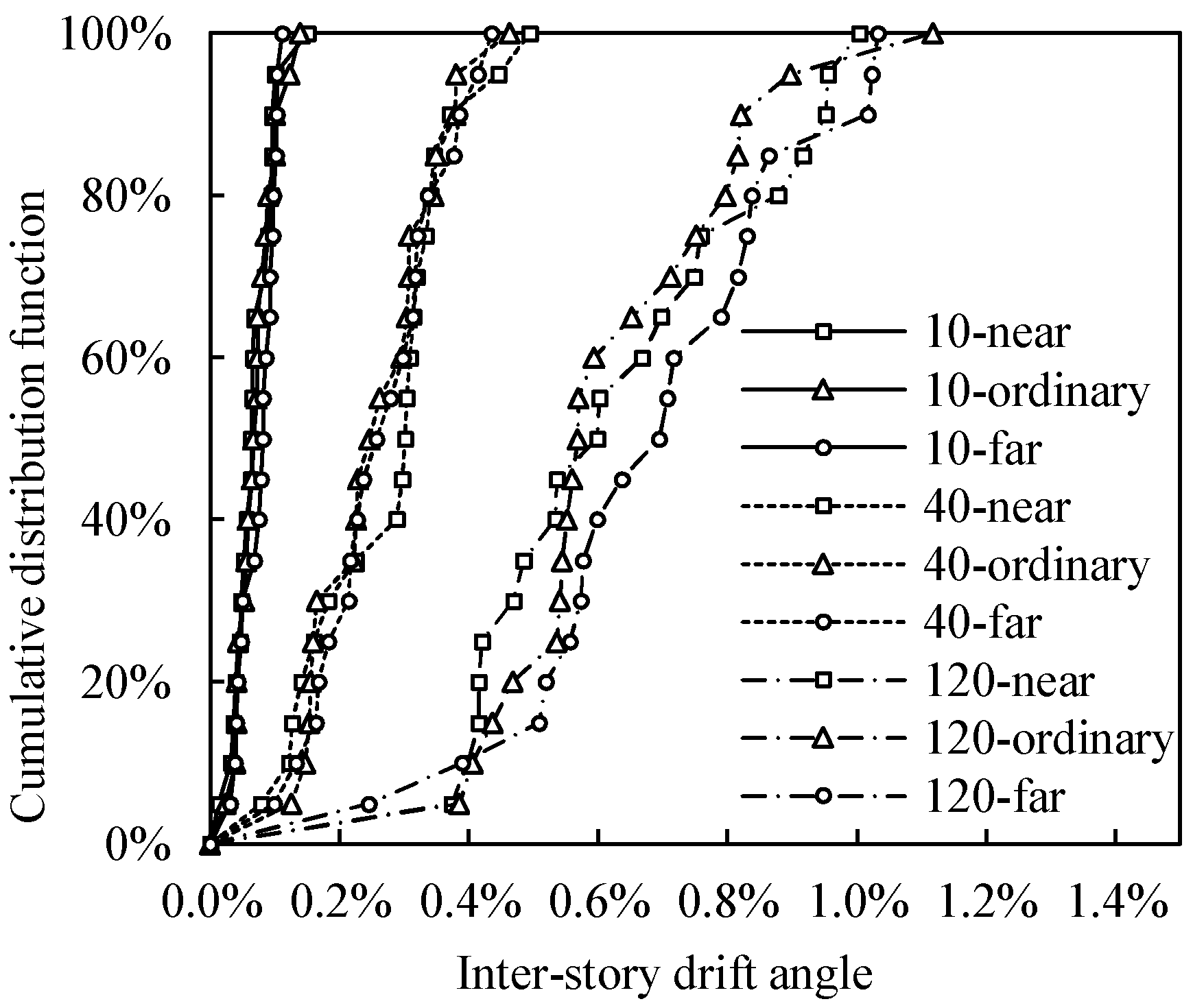
Inter-story drift angle, a common parameter in seismic response analysis, was adopted to assess structural damage. To understand its overall probability distribution, the cumulative distribution function (CDF) was calculated. The CDF integrates the probability density function and describes the probability of a random variable (X) falling within a specific range. The formulation is shown in the following equation.
Figure 4 shows the cumulative distribution function of the structural inter-story drift angle in this condition. From Figure 4, it can be observed that the distribution range of structural response is not significantly affected by different rupture distances under seismic conditions with the same PGV amplitude.
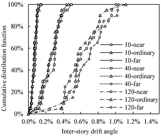
Figure 4.
Cumulative distribution function of inter-story drift angle for model under different ground motion intensities with Vs20 = 280 m/s.
With higher seismic intensity, the structural response becomes more dispersed and the effectiveness of the relationship between PGV and structural response weakens. Taking near-field seismic conditions as an example, when the PGV is 10 cm/s, the maximum inter-story drift angle is 0.151%, the minimum is 0.014%, and the range is 0.137%. At this moment, the difference between the maximum and minimum values is not significant. When the PGV is 40 cm/s, the maximum inter-story drift angle is 0.495%, the minimum is 0.080%, and the range is 0.415%. When PGV increases to 120 cm/s, the maximum inter-story drift angle is 1.004%, the minimum is 0.374%, and the range is 0.630%.
Therefore, under strong earthquake conditions, traditional single intensity indicators are insufficient to describe the seismic responses.
4.2. Correlation between the Severest Parameters and Structural Response under Different Intensities
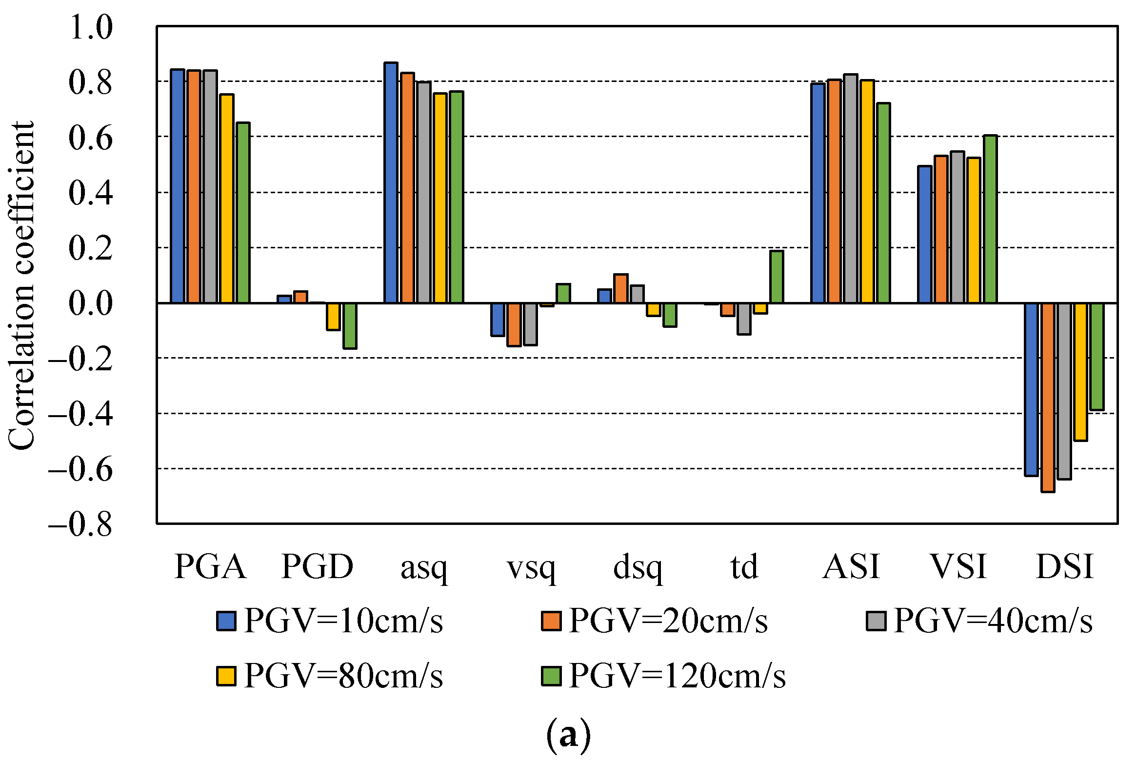
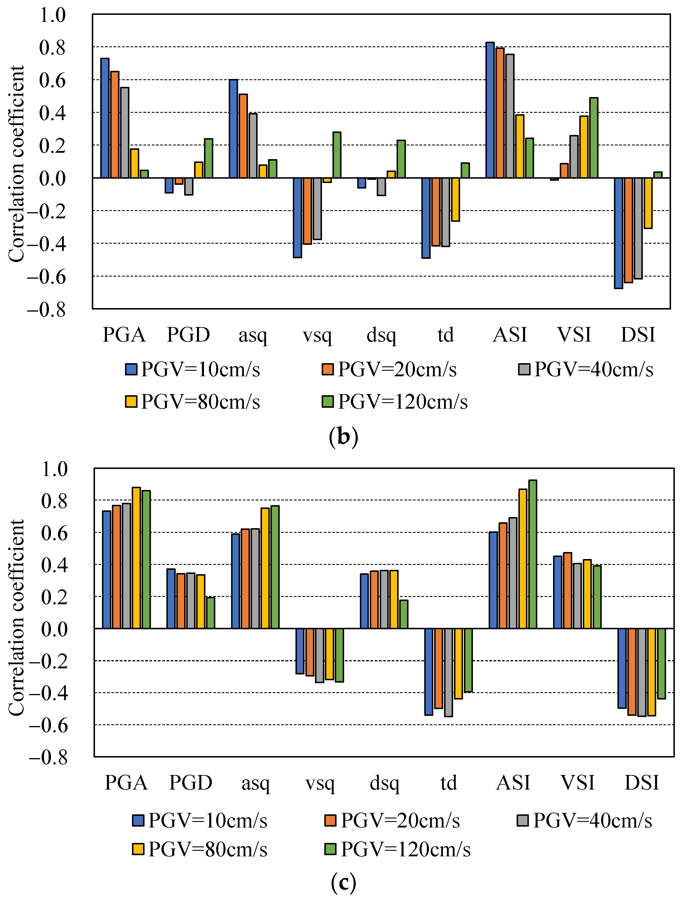
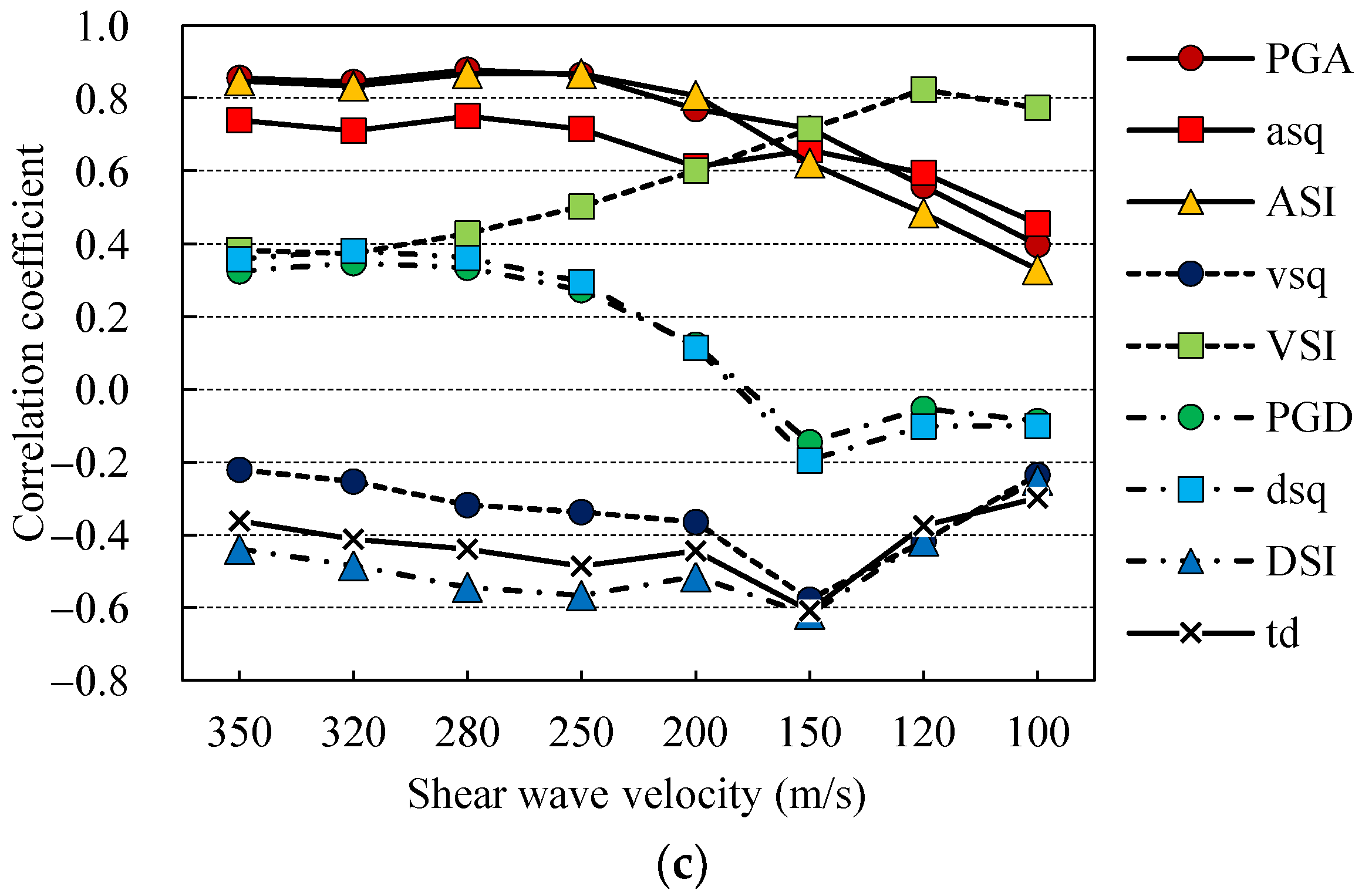
Based on the same amplitude of PGV, we analyzed the applicability of the severest parameters for describing structural seismic response through calculation of correlation coefficients, then examined the trend of correlation coefficients with the changes in seismic intensity. The correlation between the structural response and the severest parameters at different seismic intensities was calculated, and the results are shown in Figure 5. In these conditions, the station site was modeled with a soil shear wave velocity (Vs20) of 280 m/s.
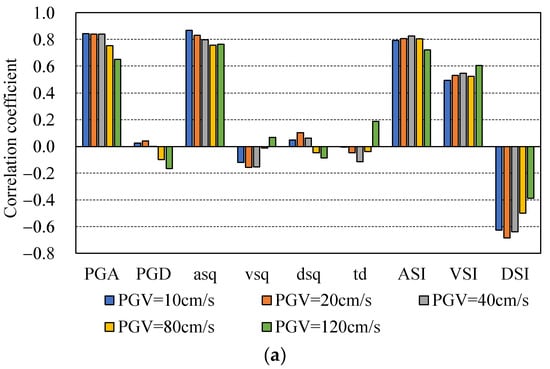
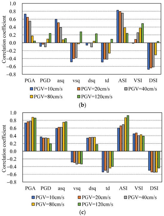
Figure 5.
Correlation coefficients between structural response and the severest ground motion parameter under different intensities with a shear wave velocity of 280 m/s: (a) near-field earthquake (R < 20 km); (b) ordinary earthquake (30 km < R < 70 km); (c) far-field earthquake (R > 80 km).
It can be observed that under near-field seismic conditions and when the PGV of the input seismic motions is 10 cm/s, the asq has the strongest correlation with the structural response and the correlation coefficient is 0.867. When the PGV increases to 20 cm/s and 40 cm/s, PGA shows the highest correlation with structural response, with correlation coefficients of 0.840 and 0.839, respectively. When PGV is 80 cm/s, ASI exhibits the highest correlation, with a correlation coefficient of 0.803. When PGV is 120 cm/s, the highest correlation is with asq, with a correlation coefficient of 0.763.
Under ordinary seismic conditions, ASI has the strongest correlation with structural response when the PGV is 10 cm/s, 20 cm/s, and 40 cm/s. The correlation coefficients for ASI in these three conditions are 0.828, 0.792, 0.755 respectively. Compared to ASI, the correlation coefficients for PGA and asq are relatively low, with values below 0.75. In particular, when PGV is 40 cm/s the correlation coefficient of asq is less than 0.4. When PGV increases to 80 cm/s, ASI demonstrates the highest correlation, with a correlation coefficient of 0.384. When PGV is 120 cm/s, VSI demonstrates the strongest correlation, with a correlation coefficient of 0.489.
Under far-field seismic conditions, PGA shows the highest correlation with structural response when PGV rises from 10 cm/s to 20 cm/s and 40 cm/s. Their corresponding correlation coefficients are 0.732, 0.766, and 0.779 respectively, while the correlation coefficients for asq and ASI are lower than 0.7. When PGV is 80 cm/s, PGA shows the highest correlation, with a correlation coefficient of 0.878. When PGV is 120 cm/s, the highest correlation is with ASI, with a correlation coefficient of 0.926.
As the seismic intensity increases, the maximum correlation coefficients of the severest parameter for near-field seismic conditions show a decreasing trend, though still exhibiting relatively high correlation overall. The maximum correlation coefficients for ordinary seismic conditions significantly decrease, with an absolute value less than 0.6, indicating a lack of correlation between the parameters and structural response. The maximum correlation coefficients for far-field seismic conditions show an increasing trend, exhibiting high correlation.
4.3. Correlation between the Severest Parameters and Structural Response at Different Sites
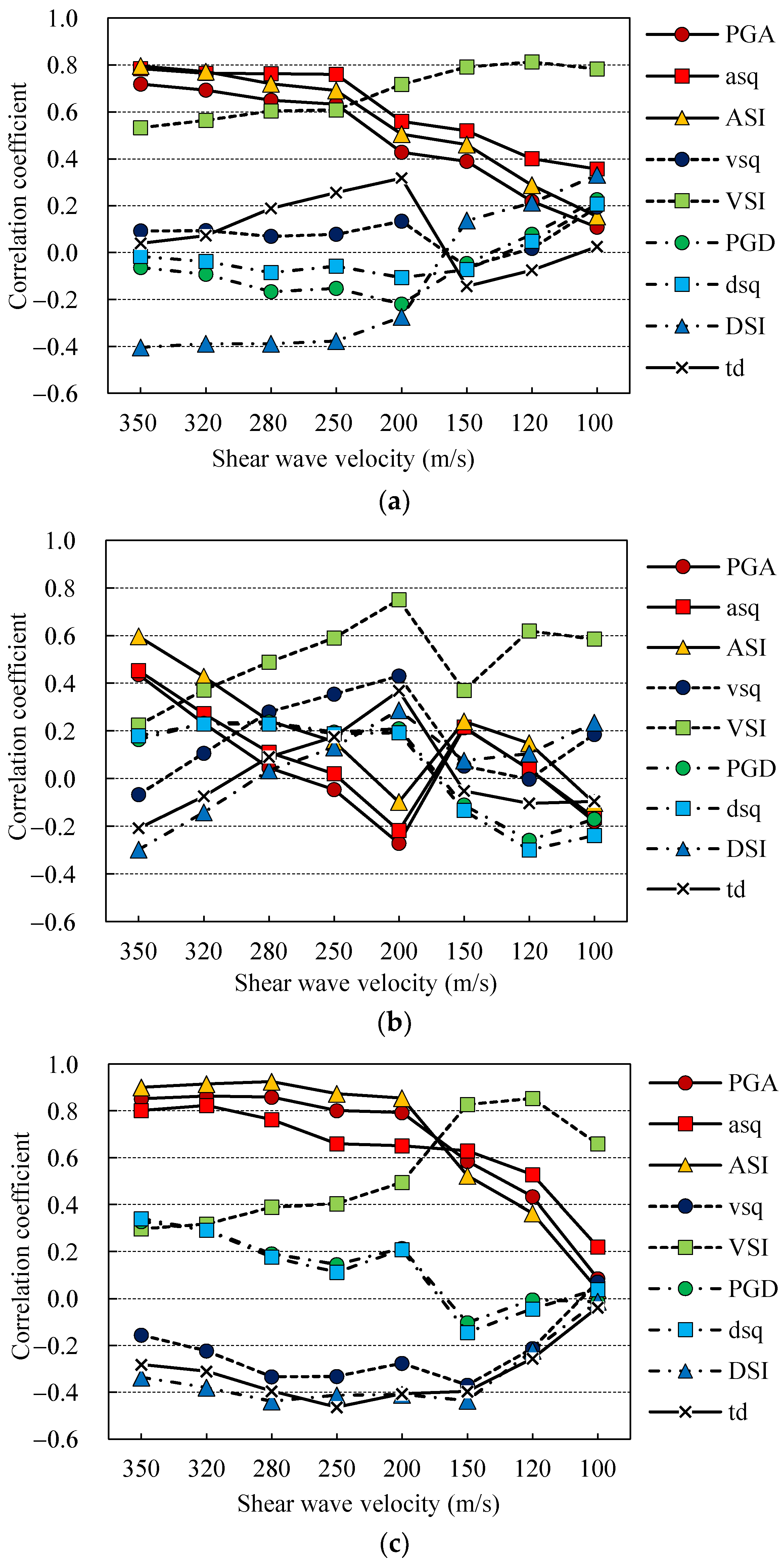
In order to analyze the influence of the site on the seismic damage capacity, we examined the correlation coefficients between structural response and the severest parameters for eight site conditions, including Class II sites with shear wave velocities of 350 m/s, 320 m/s, 280 m/s, 250 m/s, and 200 m/s and Class III sites with shear wave velocities of 150 m/s, 120 m/s, and 100 m/s. The PGVs of the input seismic motions were 120 cm/s and 80 cm/s, respectively. The results of the calculation are shown in Figure 6 and Figure 7.
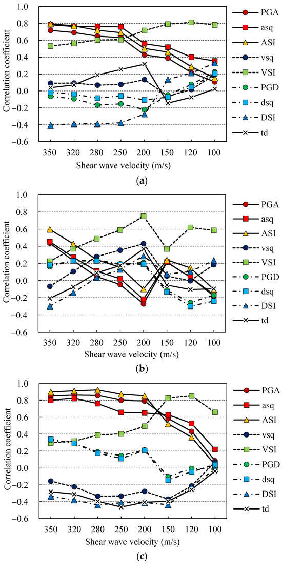
Figure 6.
Correlation coefficients between structural response and the severest parameter under different shear wave velocities with PGV = 120 cm/s: (a) near-field earthquake (R < 20 km); (b) ordinary earthquake (30 km < R < 70 km); (c) far-field earthquake (R > 80 km).
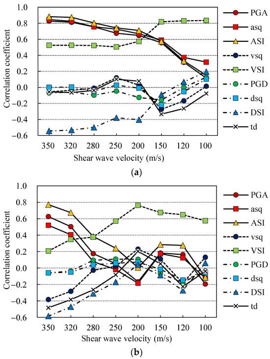
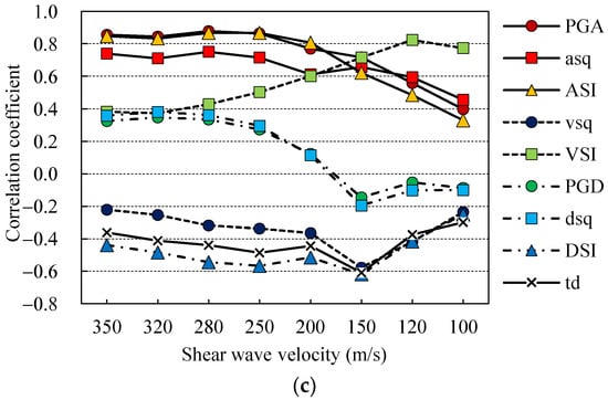
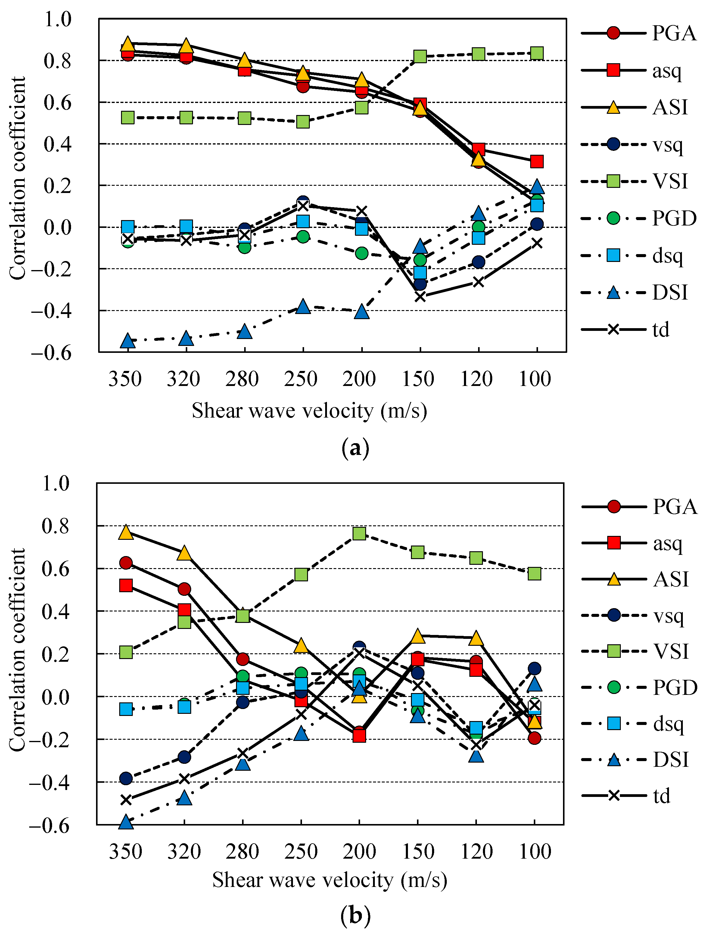
Figure 7.
Correlation coefficient between structural response and the severest parameter under different shear wave velocities with PGV = 80 cm/s: (a) near-field earthquake (R < 20 km); (b) ordinary earthquake (30 km < R < 70 km); (c) far-field earthquake (R > 80 km).
According to Figure 6, under near-field seismic conditions, asq has the highest correlation with structural response when soil shear wave velocities range from 250 m/s to 350 m/s, with the correlation coefficients fluctuating around 0.8. The correlation coefficients for ASI and PGA are high as well, though lower than asq. When shear wave velocity ranges from 100 m/s to 200 m/s, VSI shows the highest correlation. Their corresponding correlation coefficients are 0.783, 0.813, 0.792, and 0.717, respectively. In these conditions, the distribution range of the maximum correlation coefficient is between 0.7 and 0.85.
Under ordinary seismic conditions, when the soil shear wave velocity ranges from 320 m/s to 350 m/s, ASI has the highest correlation with structural response. In other conditions, VSI emerges has the highest correlation with structural response. In these conditions, the distribution range of the maximum correlation coefficient is between 0.4 and 0.8, with significant fluctuations influenced by shear wave velocity.
Under far-field seismic conditions, when the soil shear wave velocity ranges from 200 m/s to 350 m/s, the three most strongly correlated parameters are PGA, asq, and ASI. Among them, ASI has the highest correlation coefficients, which fluctuate around 0.9. When the soil shear wave velocity ranges from 100 m/s to 150 m/s, VSI shows the highest correlation with structural response. Their corresponding correlation coefficients are 0.659, 0.854, and 0.828, respectively. In these conditions, the distribution range of the maximum correlation coefficient is between 0.65 and 0.95.
According to the Figure 7, under near-field seismic conditions, ASI has the highest correlation with structural response when soil shear wave velocities range from 200 m/s to 350 m/s. Their corresponding correlation coefficients are 0.709, 0.740, 0.803, 0.872, and 0.881, respectively. The correlation coefficients of PGA and asq are slightly lower than ASI, with a very small difference. When soil shear wave velocity ranges from 100 m/s to 150 m/s, VSI shows the highest correlation, with correlation coefficients fluctuating around 0.8. In these conditions, the distribution range of the maximum correlation coefficient is between 0.7 and 0.9.
Under ordinary seismic conditions, the situation is similar with Figure 6b. The distribution range of the maximum correlation coefficient is between 0.55 and 0.8, with significant fluctuations influenced by shear wave velocity.
Under far-field seismic conditions, when the soil shear wave velocity ranges from 200 m/s to 350 m/s, PGA and ASI exhibit the highest correlation. Their correlation coefficients have similar values and are greater than 0.8. When the soil shear wave velocity ranges from 100 m/s to 150 m/s, VSI shows the highest correlation with structural response. Their corresponding correlation coefficients are 0.773, 0.823, and 0.717, respectively. In these conditions, the distribution range of the maximum correlation coefficient is between 0.7 and 0.9.
Based on the results of the above analysis, the parameters that performed well in most cases were chosen. Therefore, with the same amplitude of PGV for input motions, ASI can be used as the severest parameter for predicting seismic damage capacity in Class II sites. In Class III sites, VSI can be used as the severest parameter.
4.4. Ranking of Seismic Damage Capacity
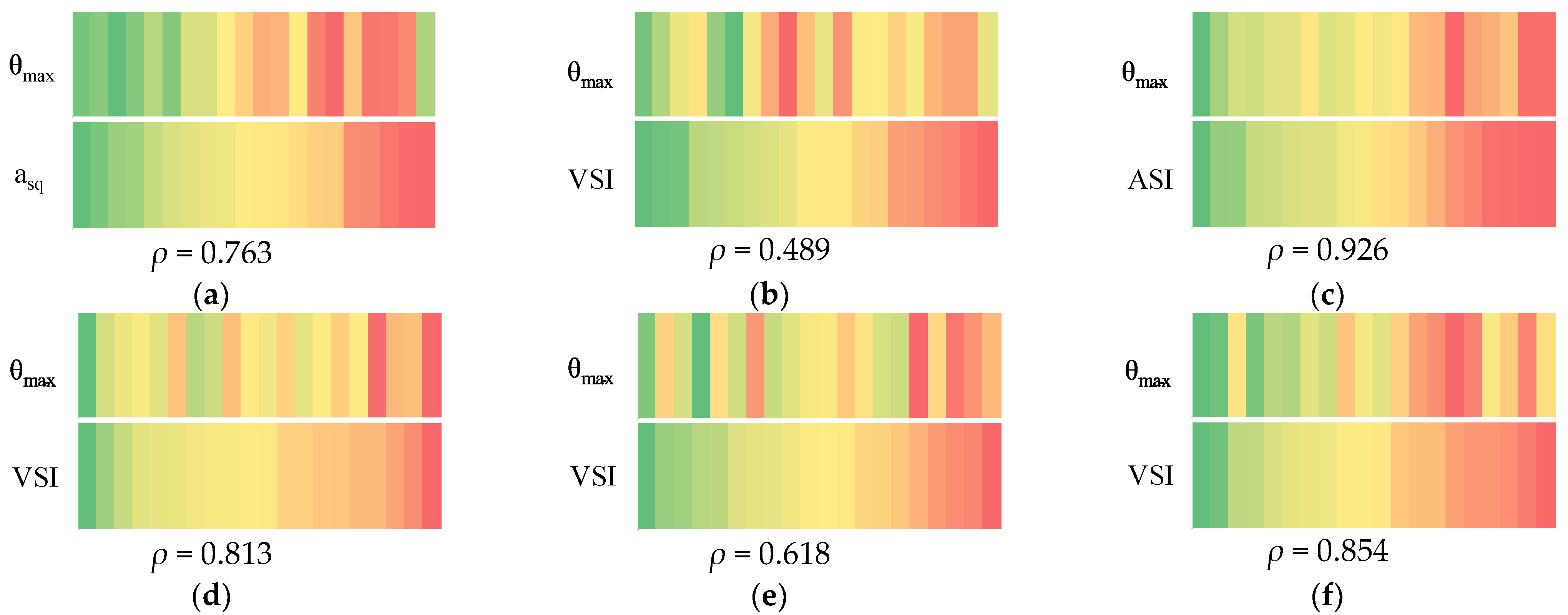
In order to visually analyze the applicability of ranking seismic damage capacity based on the severest parameter, as shown in Figure 8, the seismic records were sorted according to the size of the severest parameters. Six calculation results were selected as demonstrations.
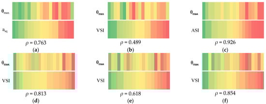
Figure 8.
The effect of assessing the seismic damage potential based on the severest parameters: (a) near-field earthquake, Vs20 = 280 m/s; (b) ordinary earthquake, Vs20 = 280 m/s; (c) far-field earthquake, Vs20 = 280 m/s; (d) near-field earthquake, Vs20 = 120 m/s; (e) ordinary earthquake, Vs20 = 120 m/s; (f) far-field earthquake, Vs20 = 120 m/s.
In the lower part of subgraph in Figure 8, the seismic records are sorted based on the values of the severest parameters. From left to right, the values of the severest parameters present an increasing trend. The seismic records are color-coded using a color mapping technique, with red indicating the highest values and green indicating the lowest values.
In the upper part of the subgraph in Figure 8, it can be seen that the sorting of seismic records remains unchanged from the lower part of subgraph. Based on the size of the inter-story drift angle, these records were recolored. Red represents the record with the highest inter-story drift angle and green represents the lowest.
The symbol ρ in the figures represents the correlation coefficient between the inter-story drift angle and the severest parameter.
As shown in Figure 8, the correlation coefficient in Figure 8c is 0.926, and the color order of the inter-story drift angle is basically the same as that of the severest parameter. In Figure 8a,d,f, the correlation coefficients are 0.763, 0.813, and 0.854, respectively, indicating that the size of the severest parameter can roughly reflect the seismic damage capacity. The correlation coefficients in Figure 8b and e are 0.489 and 0.618, respectively. It is obvious that the correspondence between the size of the severest parameters and the structural response is relatively poor. Overall, when the correlation coefficient is relatively high (greater than 0.8), the selected size of the most critical indicator can be used to rank the seismic damage capacity.
5. Conclusions
This paper establishes a finite element model of a soil–underground station structure and conducts seismic response analysis using the incremental dynamic analysis method. By analyzing the correlation between the severest parameter and the inter-layer drift angle, the paper investigates how to select the seismic motion with the maximum potential damage capacity. Additionally, the impact of various site conditions and seismic source distances is taken into account. The following conclusions are obtained:
- (1)
- As the seismic intensity increases, the structural forces show an increasing trend. The range of the maximum inter-layer drift angle of the underground structure grows from 0.137% to 0.630% when the PGV increases from 10 cm/s to 120 cm/s, and the difference in structural response significantly increases. This indicates that it is necessary to differentiate the damage capacities of different seismic motions for structures under strong seismic conditions.
- (2)
- With a high PGV amplitude of the input seismic motions, the severest parameters exhibit a high correlation with structural responses under both near-field and far-field seismic motions, with the maximum correlation coefficient exceeding 0.9. The correlation with structural responses under ordinary earthquake conditions is poor, with a maximum correlation coefficient below 0.5. Therefore, the application of the severest parameters for ranking damage capacities for different seismic motions is more suitable for near-field and far-field seismic conditions.
- (3)
- When selecting input seismic motions based on the severest parameter, the following principle can be adopted: with the same amplitude of PGV for input seismic motions, ASI can be used as the severest parameter for predicting seismic damage capacity in Class II sites. In Class III sites, VSI can be used as the severest parameter.
- (4)
- When there is a strong correlation between the severest parameter and the structural response (ρ greater than 0.8), the ranking of the severest parameter can effectively indicate the potential damage capability of seismic motions.
Author Contributions
Conceptualization, Y.L.; methodology, Y.L.; software, Y.L.; validation, Y.L.; formal analysis, Y.L.; investigation, Y.L. and H.W.; resources, Y.L.; data curation, Y.L.; writing—original draft preparation, Y.L. and H.W.; writing—review and editing, Y.L. and H.W.; visualization, Y.L.; supervision, H.W.; project administration, H.W.; funding acquisition, H.W. All authors have read and agreed to the published version of the manuscript.
Funding
This research received no external funding.
Data Availability Statement
The data presented in this study are available on request from the corresponding author. The data are not publicly available due to privacy.
Acknowledgments
We are grateful to the anonymous reviewers for their constructive comments.
Conflicts of Interest
The authors declare no conflicts of interest.
References
- Drenick, R.F. Model-free design of aseismic structures. J. Eng. Mech. Div. 1970, 96, 483–493. [Google Scholar] [CrossRef]
- Abbas, A.M.; Manohar, C.S. Investigations into critical earthquake load models within deterministic and probabilistic frameworks. Earthq. Eng. Struct. Dyn. 2002, 31, 813–832. [Google Scholar] [CrossRef]
- Takewaki, I. Nonstationary random critical excitation for acceleration response. J. Eng. Mech. 2001, 127, 544–556. [Google Scholar] [CrossRef]
- Khatibinia, M.; Gholami, H.; Kamgar, R. Optimal design of tuned mass dampers subjected to continuous stationary critical excitation. Int. J. Dyn. Control 2018, 6, 1094–1104. [Google Scholar] [CrossRef]
- Zhai, C.; Xie, L. A new approach of selecting real input ground motions for seismic design: The most unfavorable real seismic design ground motions. Earthq. Eng. Struct. Dyn. 2007, 36, 1009–1027. [Google Scholar] [CrossRef]
- Bradley, B.A. A generalized conditional intensity measure approach and holistic ground motion selection. Earthq. Eng. Struct. Dyn. 2010, 39, 1321–1342. [Google Scholar] [CrossRef]
- Bradley, B.A. Correlation of significant duration with amplitude and cumulative intensity measures and its use in ground motion selection. J. Earthq. Eng. 2011, 15, 809–832. [Google Scholar] [CrossRef]
- Li, C.; Zhai, C.; Kunnath, S.; Ji, D. Methodology for selection of the most damaging ground motions for nuclear power plant structures. Soil Dynam. Earthq. Eng. 2019, 116, 345–357. [Google Scholar] [CrossRef]
- Zhai, C.; Chang, Z.; Li, S.; Xie, L. Selection of the most unfavorable real ground motions for low-and mid-rise RC frame structures. J. Earthq. Eng. 2013, 17, 1233–1251. [Google Scholar] [CrossRef]
- Lekshmy, P.R.; Raghukanth, S.T.G. Maximum possible ground motion for linear structures. J. Earthq. Eng. 2015, 19, 938–955. [Google Scholar] [CrossRef]
- Manohar, C.S.; Sarkar, A. Critical earthquake input power spectral density function models for engineering structures. Earthq. Eng. Struct. Dyn. 1995, 24, 1549–1566. [Google Scholar] [CrossRef]
- Chen, Z.; Yu, W.; Zhu, H.; Xie, L. Ranking method of the severest input ground motion for underground structures based on composite ground motion intensity measures. Soil Dynam. Earthq. Eng. 2023, 168, 107828. [Google Scholar] [CrossRef]
- Argyroudis, S.A.; Pitilakis, K.D. Seismic fragility curves of shallow tunnels in alluvial deposits. Soil Dynam. Earthq. Eng. 2012, 35, 1–12. [Google Scholar] [CrossRef]
- Zhuang, H.; Yang, J.; Chen, S.; Dong, Z.; Chen, G. Statistical numerical method for determining seismic performance and fragility of shallow-buried underground structure. Tunn. Undergr. Space Technol. 2021, 116, 104090. [Google Scholar] [CrossRef]
- Xu, Z.; Zhuang, H.; Xia, Z.; Yang, J.; Bu, X. Study on the effect of burial depth on seismic response and seismic intensity measure of underground structures. Soil Dynam. Earthq. Eng. 2023, 166, 107782. [Google Scholar] [CrossRef]
- Padgett, J.E.; Nielson, B.G.; DesRoches, R. Selection of optimal intensity measures in probabilistic seismic demand models of highway bridge portfolios. Earthq. Eng. Struct. Dynam. 2008, 37, 711–725. [Google Scholar] [CrossRef]
- Jiang, J.; El Naggar, M.H.; Huang, W.; Xu, C.; Zhao, K.; Du, X. Seismic vulnerability analysis for shallow-buried underground frame structure considering 18 existing subway stations. Soil Dyn. Earthg. Eng. 2022, 162, 107479. [Google Scholar] [CrossRef]
- Mayoral, J.M.; Argyroudis, S.; Castanon, E. Vulnerability of floating tunnel shafts for increasing earthquake loading. Soil Dyn. Earthg. Eng. 2016, 80, 1–10. [Google Scholar] [CrossRef]
- Argyroudis, S.; Tsinidis, G.; Gatti, F.; Pitilakis, K. Effects of SSI and lining corrosion on the seismic vulnerability of shallow circular tunnels. Soil Dyn. Earthg. Eng. 2017, 98, 244–256. [Google Scholar] [CrossRef]
- Tsinidis, G.; Di Sarno, L.; Sextos, A.; Furtner, P. Optimal intensity measures for the structural assessment of buried steel natural gas pipelines due to seismically-induced axial compression at geotechnical discontinuities. Soil Dyn. Earthg. Eng. 2020, 131, 106030. [Google Scholar] [CrossRef]
- Corigliano, M.; Lai, C.G.; Barla, G. Seismic vulnerability of rock tunnels using fragility curves. In Proceedings of the 11th ISRM Congress, Lisbon, Portugal, 9–13 July 2007. [Google Scholar]
- Huang, Z.; Pitilakis, K.; Argyroudis, S.; Tsinidis, G.; Zhang, D. Selection of optimal intensity measures for fragility assessment of circular tunnels in soft soil deposits. Soil Dynam. Earthq. Eng. 2021, 145, 106724. [Google Scholar] [CrossRef]
- Liu, T.; Chen, Z.; Yuan, Y.; Shao, X. Fragility analysis of a subway station structure by incremental dynamic analysis. Adv. Struct. Eng. 2017, 20, 1111–1124. [Google Scholar] [CrossRef]
- Zhang, C.; Zhao, M.; Zhong, Z.; Du, X. Optimum intensity measures for probabilistic seismic demand model of subway stations with different burial depths. Soil Dynam. Earthq. Eng. 2022, 154, 107138. [Google Scholar] [CrossRef]
- Kia, A.; Şensoy, S. Assessment the Effective Ground Motion Parameters on Seismic Performance of R/C Buildings Using Artificial Neural Network. 2014. Available online: http://hdl.handle.net/11129/2451 (accessed on 15 April 2016).
- Ozmen, H.B. Developing hybrid parameters for measuring damage potential of earthquake records: Case for RC building stock. Bull. Earthq. Eng. 2017, 15, 3083–3101. [Google Scholar] [CrossRef]
- Morfidis, K.; Kostinakis, K. Seismic parameters’ combinations for the optimum prediction of the damage state of R/C buildings using neural networks. Adv. Eng. Softw. 2017, 106, 1–16. [Google Scholar] [CrossRef]
- Kostinakis, K.; Athanatopoulou, A.; Morfidis, K. Correlation between ground motion intensity measures and seismic damage of 3D R/C buildings. Eng. Struct. 2015, 82, 151–167. [Google Scholar] [CrossRef]
- Luco, N.; Cornell, C.A. Structure-specific scalar intensity measures for near-source and ordinary earthquake ground motions. Earthq. Spectra 2007, 23, 357–392. [Google Scholar] [CrossRef]
- Iida, H.; Hiroto, T.; Yoshida, N.; Iwafuji, M. Damage to Daikai subway station. Soils Found. 1996, 36, 283–300. [Google Scholar] [CrossRef] [PubMed]
- Zhong, Z.; Shen, Y.; Zhao, M.; Li, L.; Du, X.; Hao, H. Seismic fragility assessment of the Daikai subway station in layered soil. Soil Dynam. Earthq. Eng. 2020, 132, 106044. [Google Scholar] [CrossRef]
- Bray, J.D.; Rodriguez-Marek, A. Characterization of forward-directivity ground motions in the near-fault region. Soil Dynam. Earthq. Eng. 2004, 24, 815–828. [Google Scholar] [CrossRef]
- Li, S.; Xie, L. Progress and trend on near-field problems in civil engineering. Acta Seismol. Sin. 2007, 20, 105–114. [Google Scholar] [CrossRef]
- Zhang, H.; Lian, M.; Su, M.; Cheng, Q. Lateral force distribution in the inelastic state for seismic design of high-strength steel framed-tube structures with shear links. Struct. Design Tall Spec. Build. 2020, 29, e1801. [Google Scholar] [CrossRef]
- Vamvatsikos, D.; Cornell, C.A. Incremental dynamic analysis. Earthq. Eng. Struct. Dyn. 2002, 31, 491–514. [Google Scholar] [CrossRef]
- Buratti, N.A. comparison of the performances of various ground–motion intensity measures. In Proceedings of the 15th World Conference on Earthquake Engineering, Lisbon, Portugal, 24–28 September 2012. [Google Scholar]
- Nguyen, D.D.; Lee, T.H.; Phan, V.T. Optimal earthquake intensity measures for probabilistic seismic demand models of base-isolated nuclear power plant structures. Energies 2021, 14, 5163. [Google Scholar] [CrossRef]
Disclaimer/Publisher’s Note: The statements, opinions and data contained in all publications are solely those of the individual author(s) and contributor(s) and not of MDPI and/or the editor(s). MDPI and/or the editor(s) disclaim responsibility for any injury to people or property resulting from any ideas, methods, instructions or products referred to in the content. |
© 2024 by the authors. Licensee MDPI, Basel, Switzerland. This article is an open access article distributed under the terms and conditions of the Creative Commons Attribution (CC BY) license (https://creativecommons.org/licenses/by/4.0/).