
Case Study of Space Optimization Simulation of Existing Office Buildings Based on Thermal Buffer Effect


Abstract
1. Introduction
2. Research Overview and Methodology
2.1. Research Framework
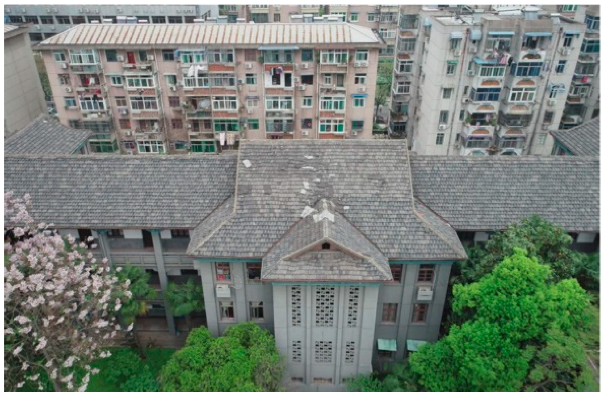
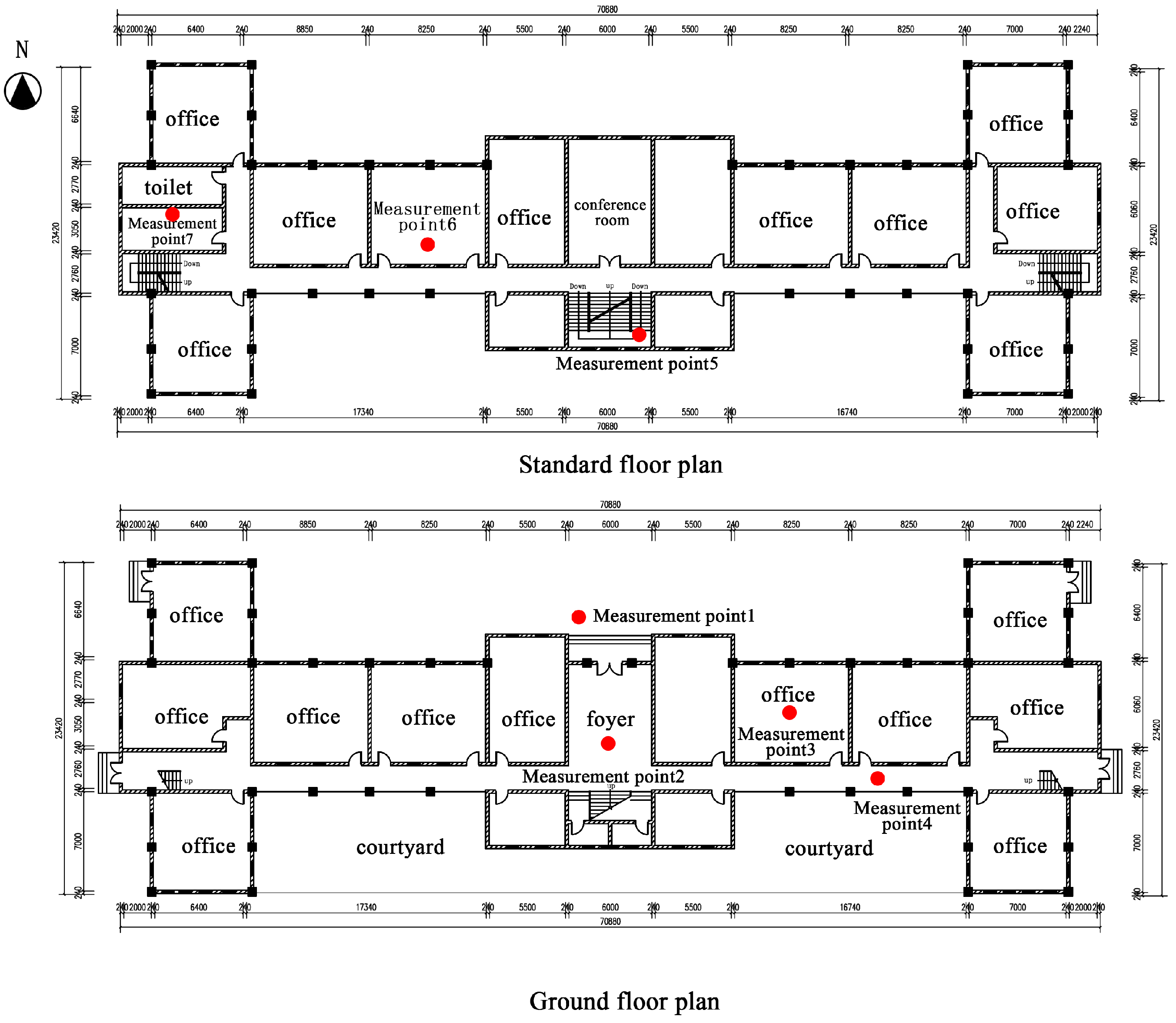
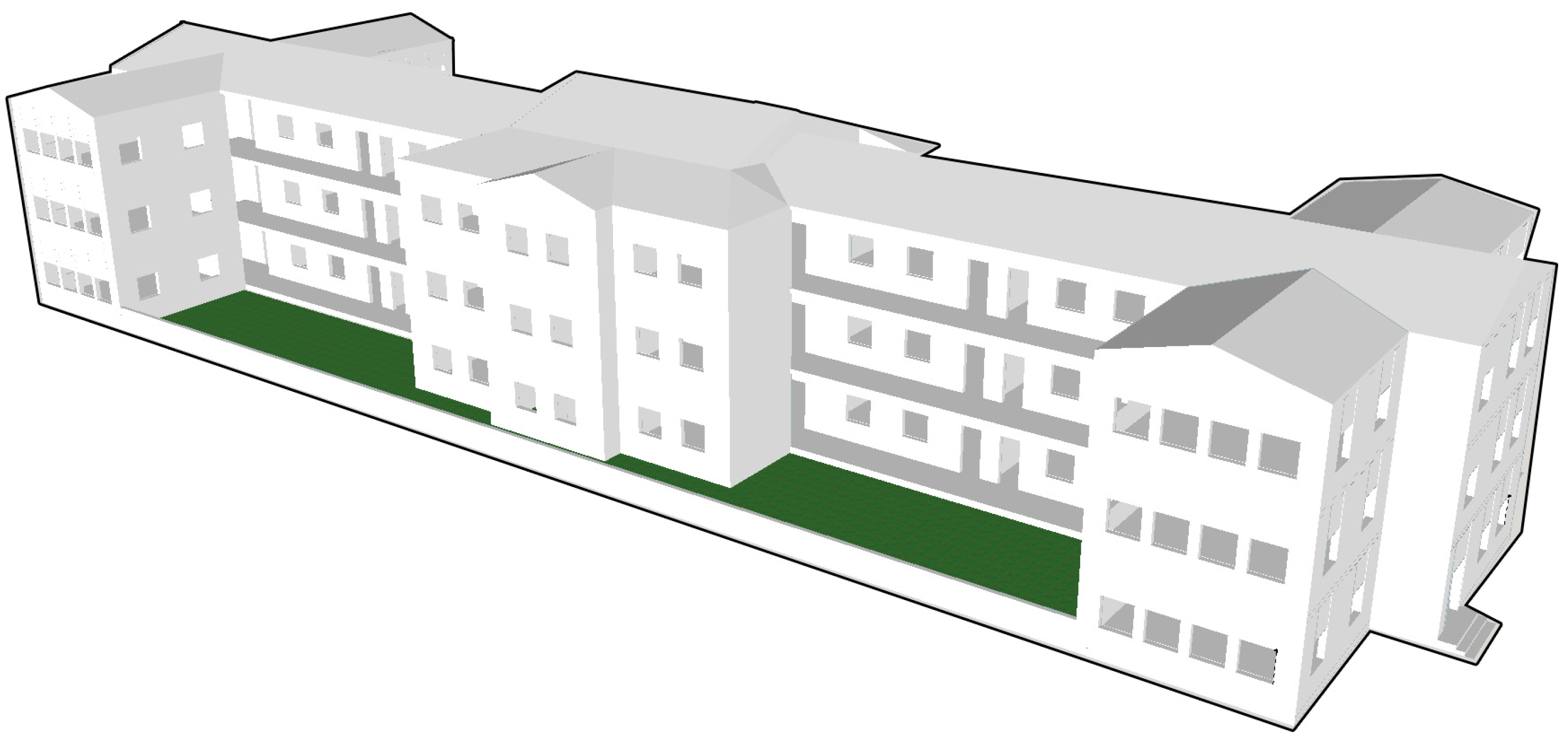
2.2. Research Area and Object
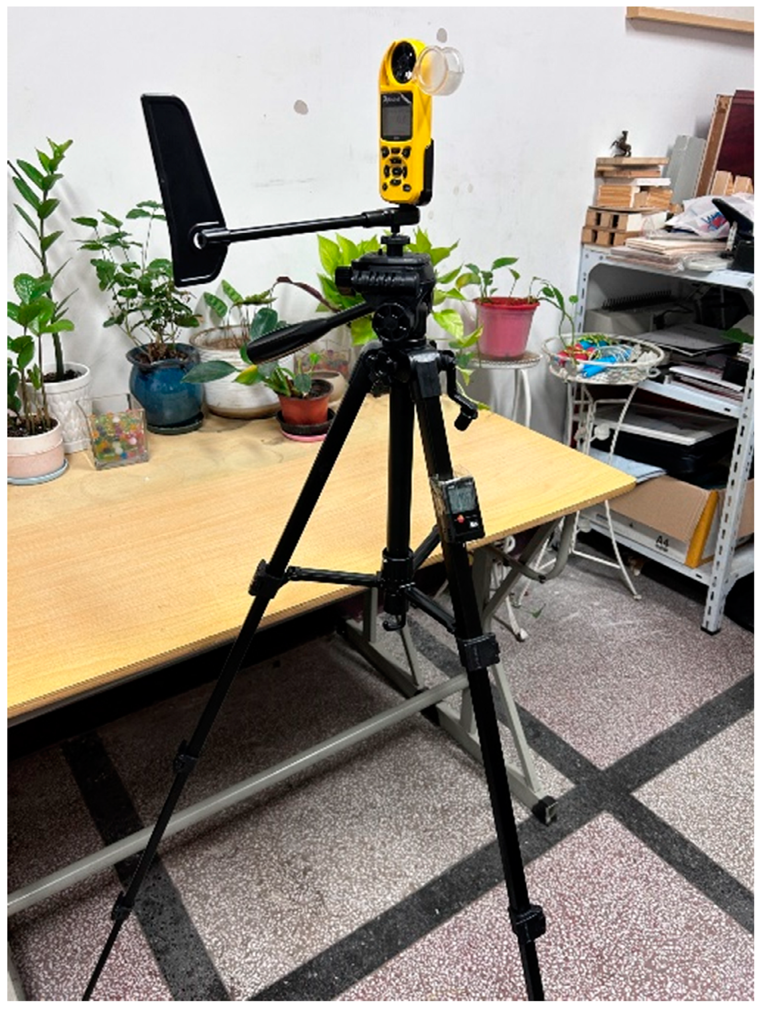
2.3. Measurement Method
2.4. Analogy Method
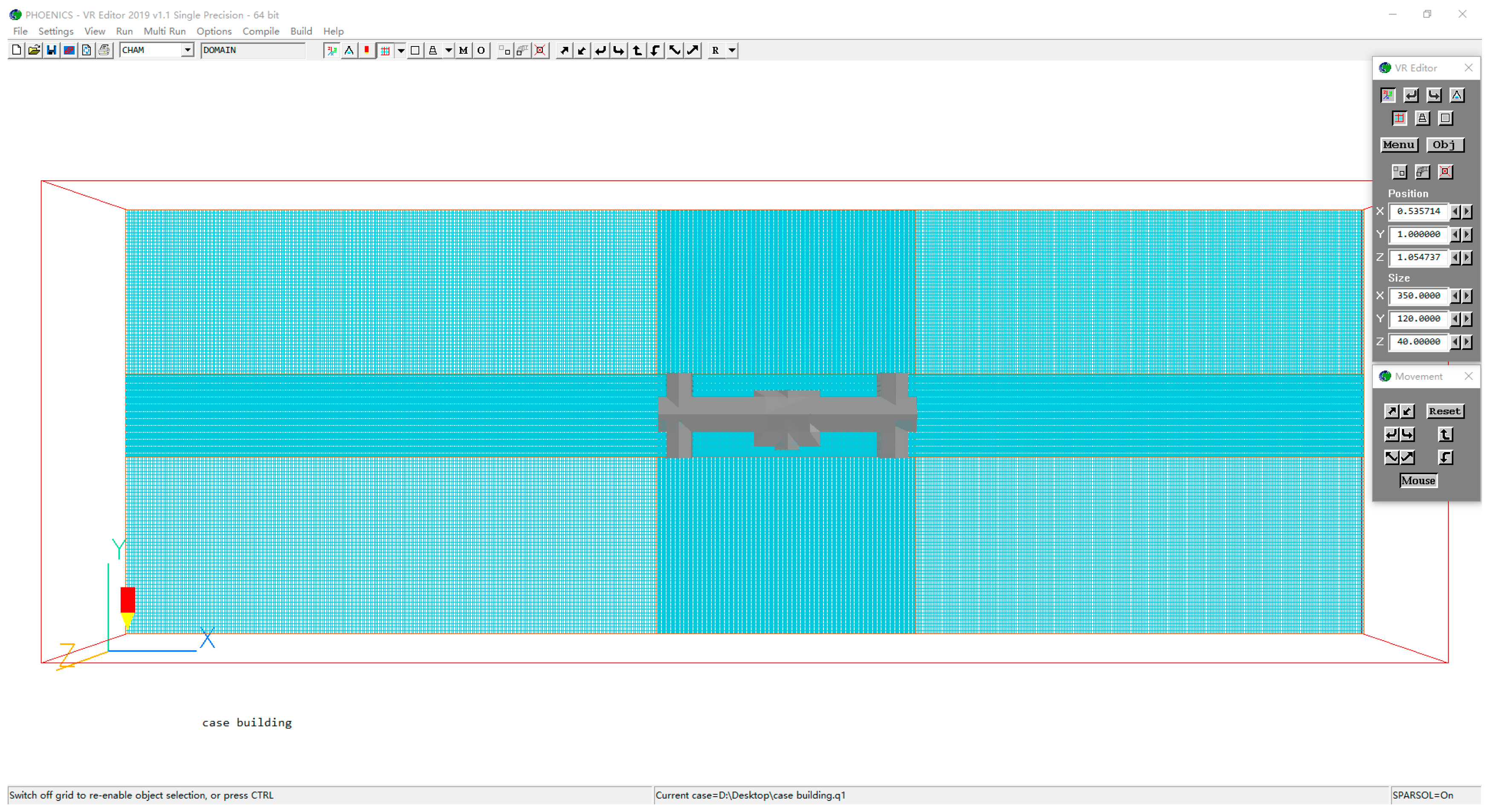
2.4.1. Boundary Condition Setting
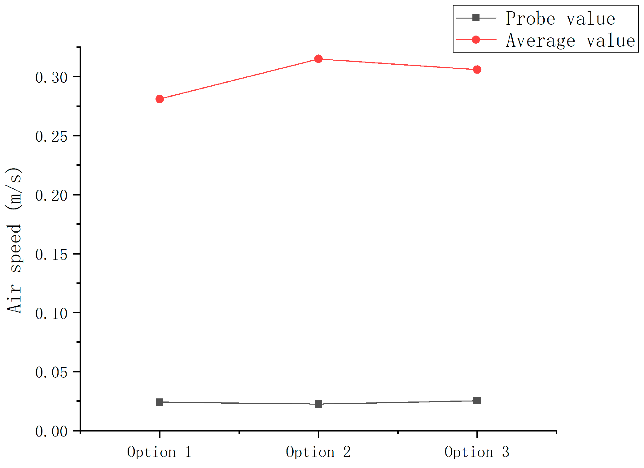
2.4.2. Grid Division and Convergence Calculation
2.5. Data Processing and Evaluation
2.5.1. Data Processing
2.5.2. Evaluating Indicator
3. Test Results and Analysis
3.1. Test Results
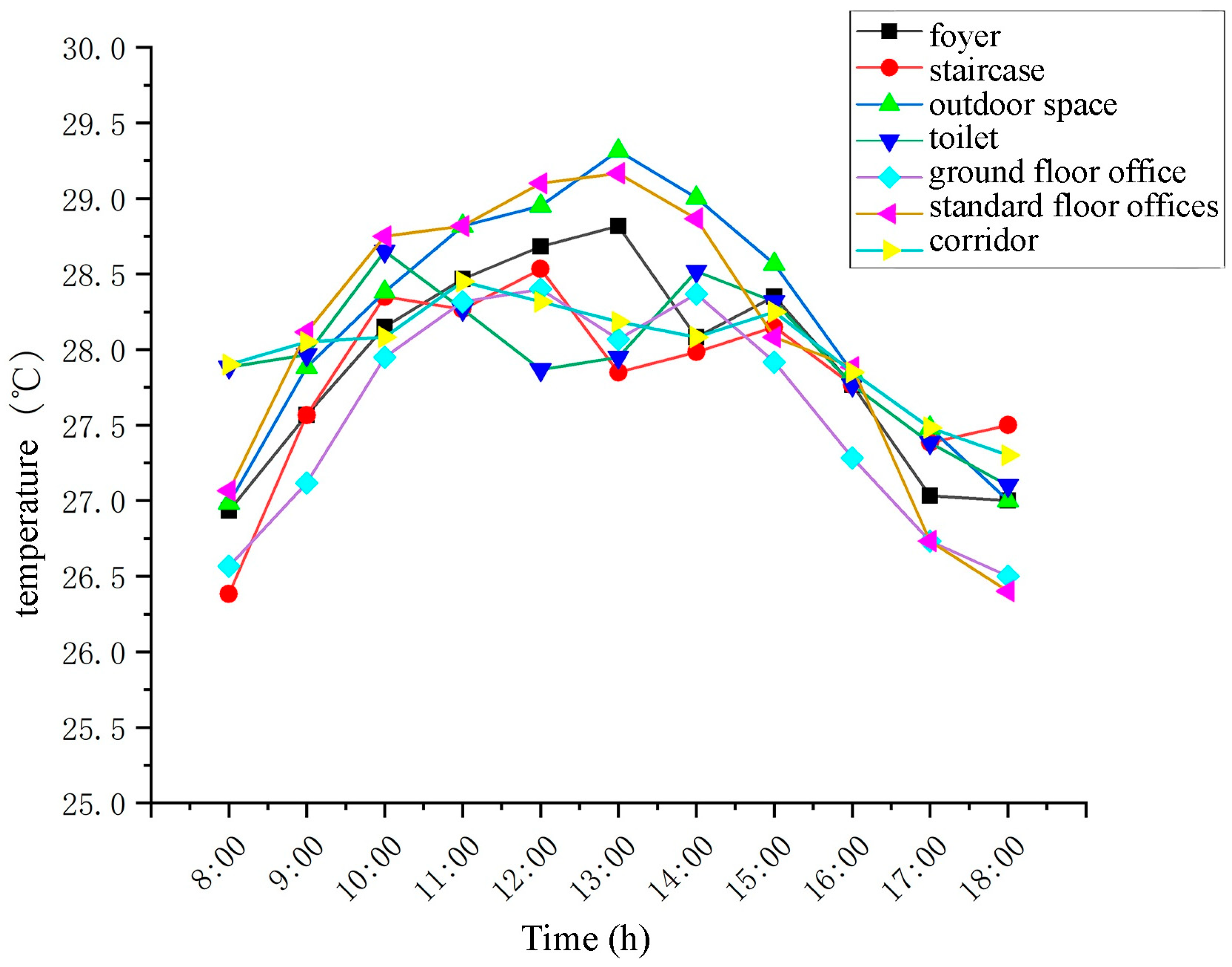
3.1.1. Indoor Temperature
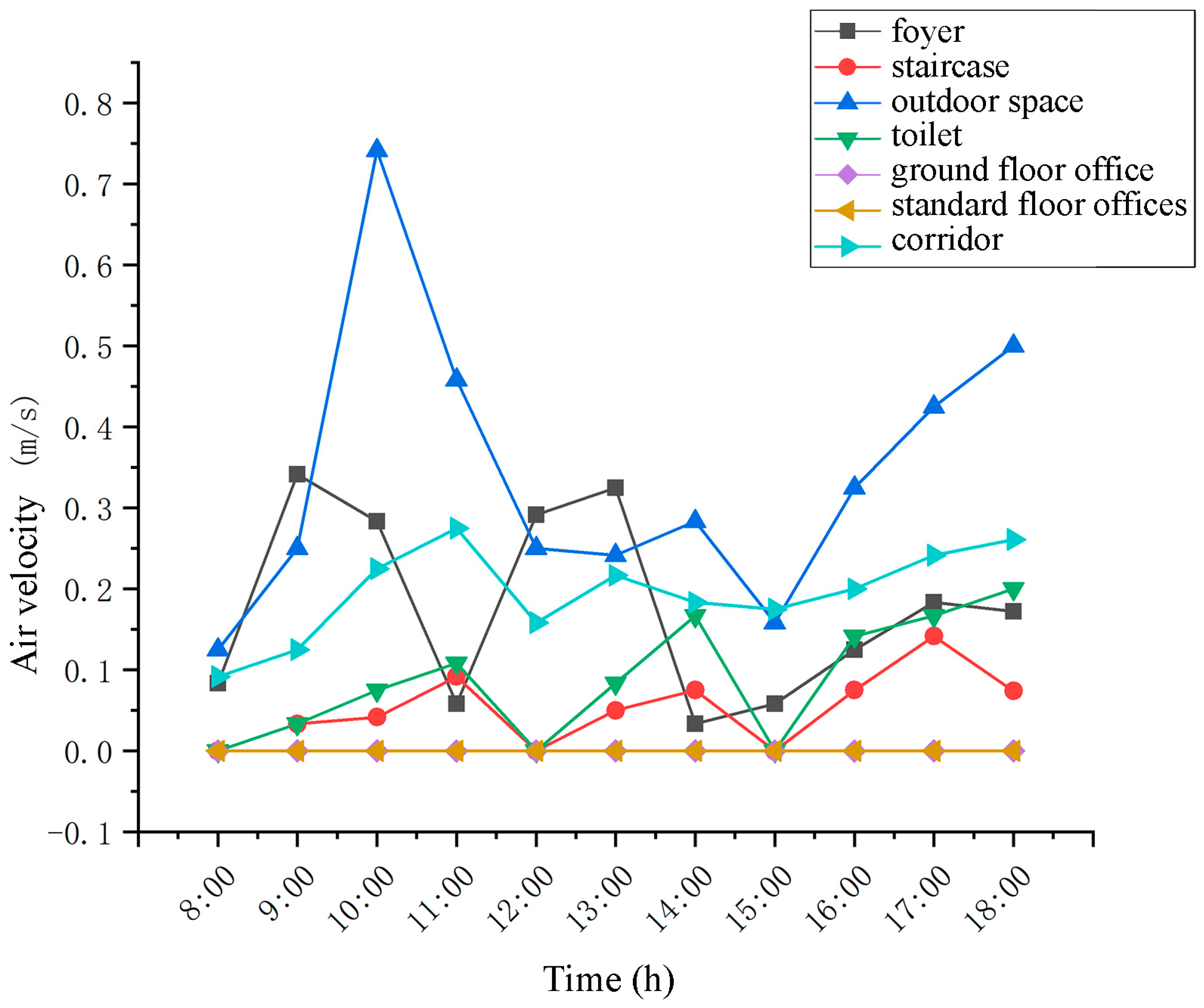
3.1.2. Indoor Air Speed
3.2. Analysis of the Test Results
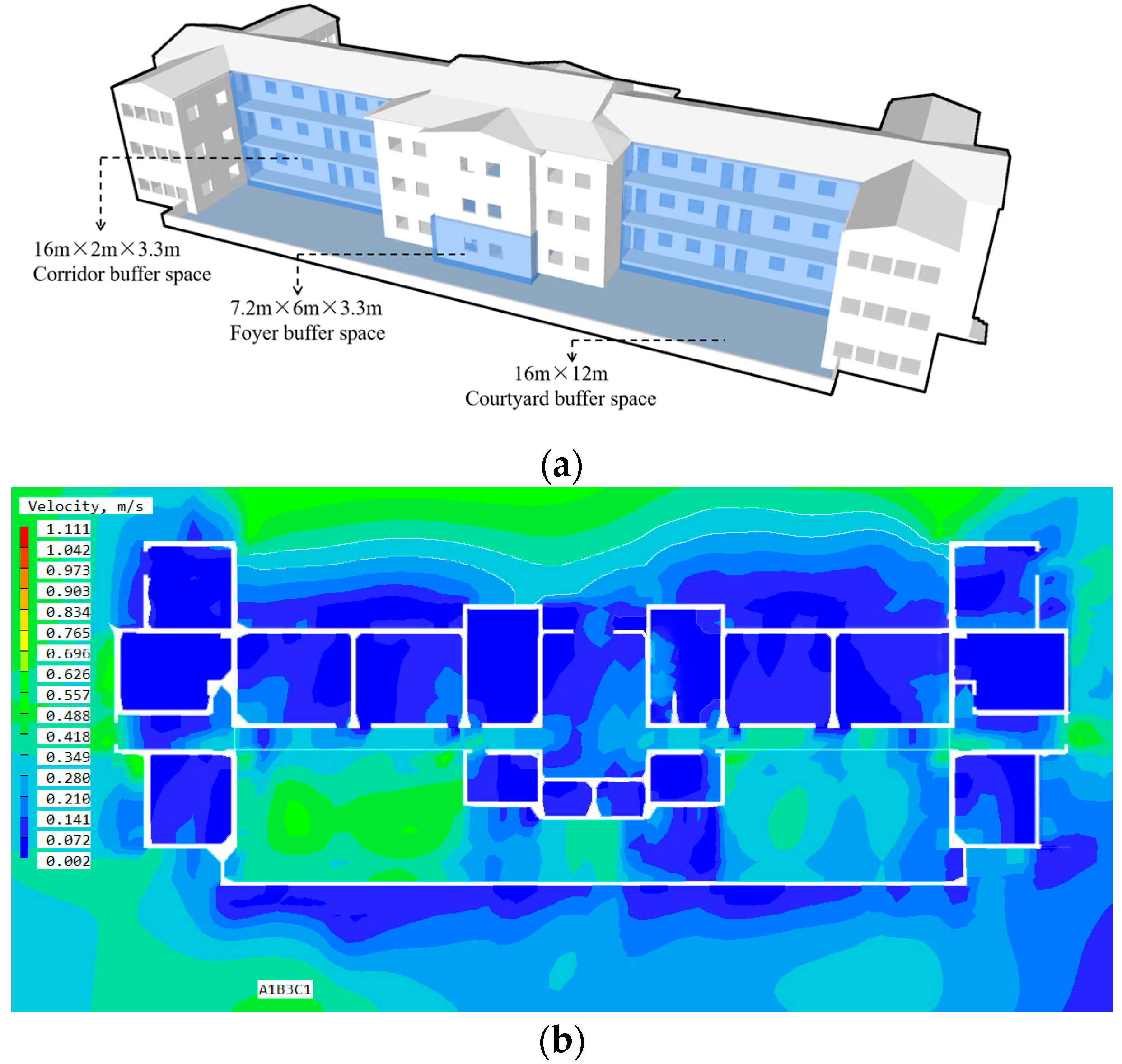
4. Buffer Space Optimization Simulation
4.1. Indicator Selection and Variable Settings
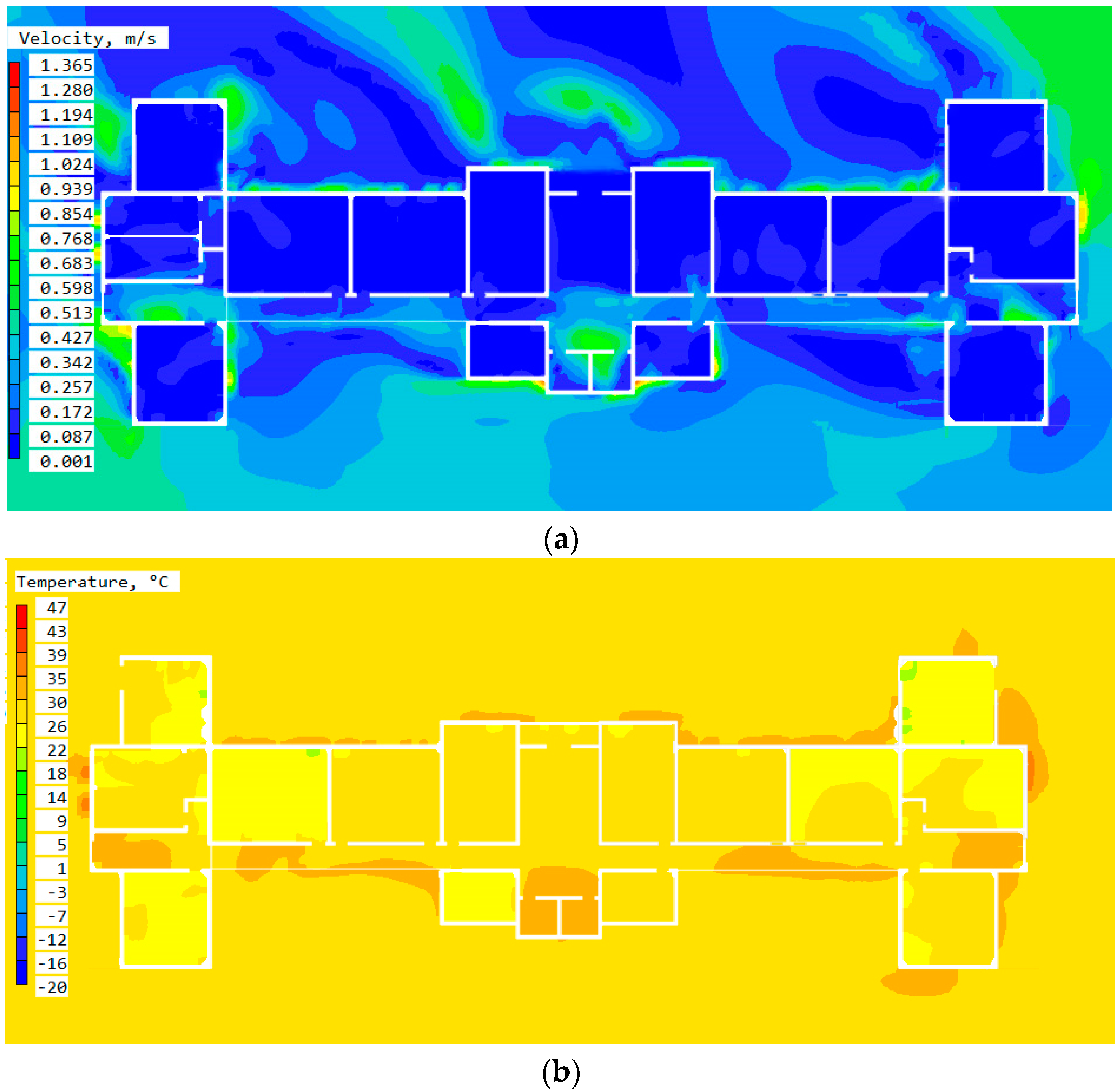
4.2. Simulation and Analysis of the Original Model
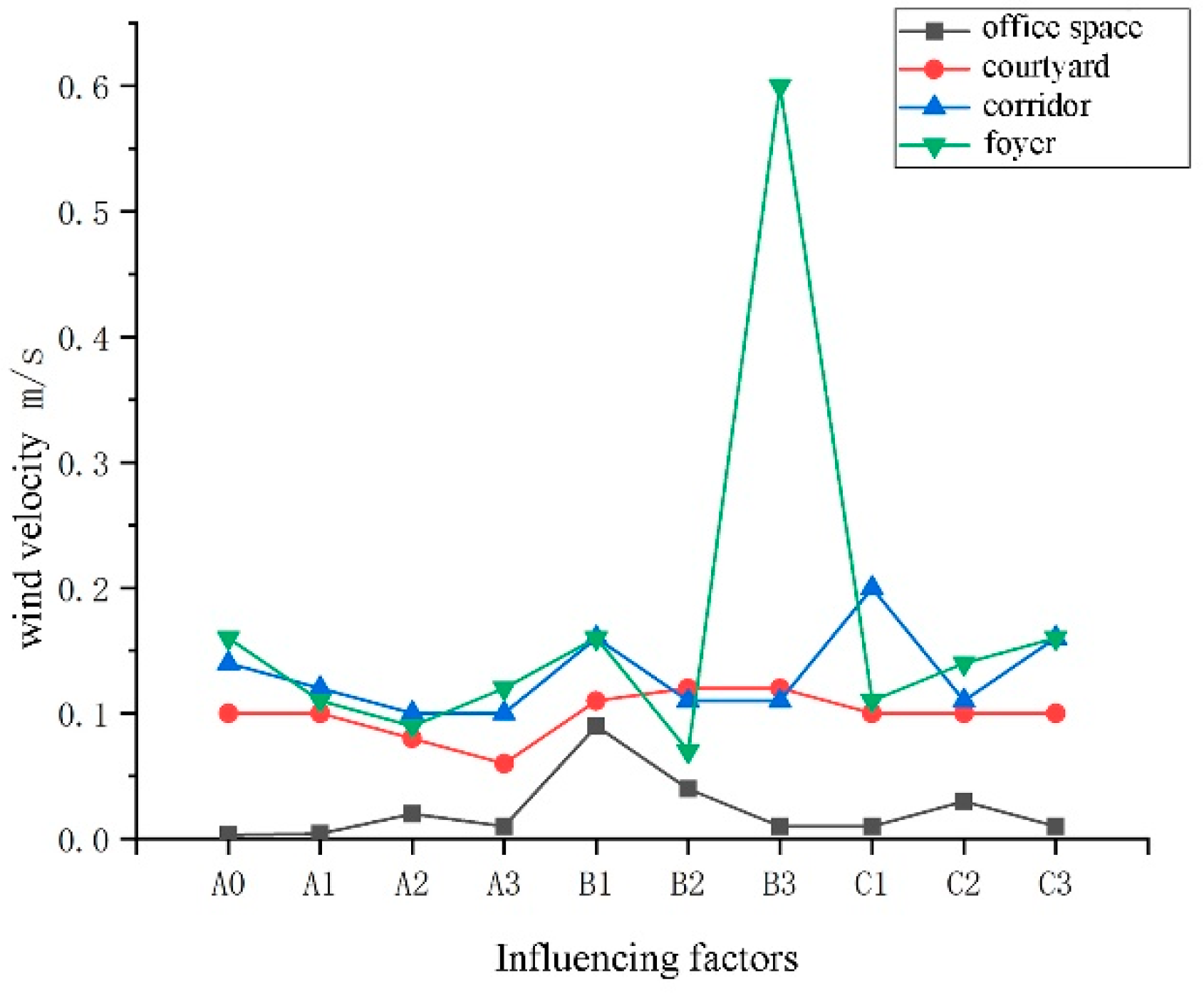
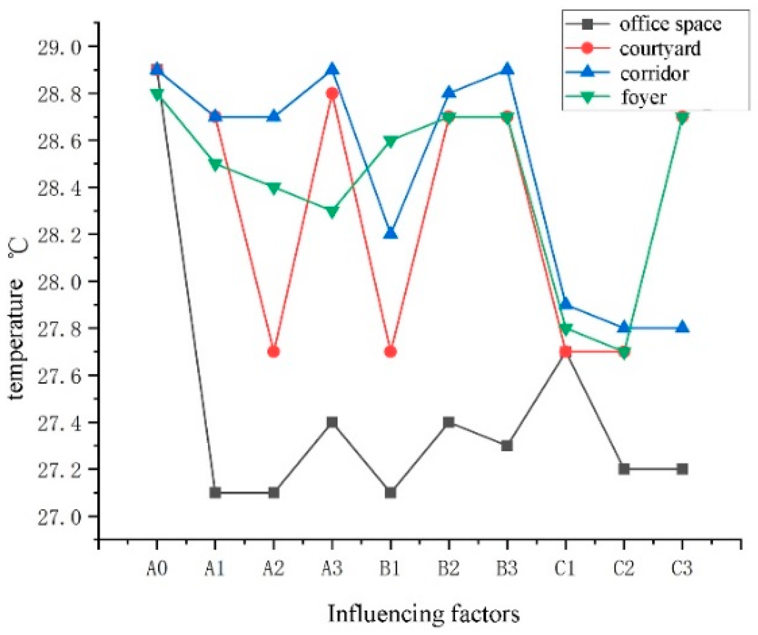
4.3. Single-Variable Simulation Analysis
4.4. Multivariate Combined Simulation Analysis
4.4.1. Orthogonal Experimental Design
4.4.2. Significance Analysis of the Influencing Factors
- Range Analysis
- 2.
- Multivariate analysis of variance
5. Discussion
6. Conclusions
Author Contributions
Funding
Data Availability Statement
Conflicts of Interest
References
- International Energy Agency Buildings Home Page. Available online: https://www.iea.org/energy-system/buildings (accessed on 10 November 2023).
- The 14th Five-Year Plan for Building Energy Conservation and Green Building Development; Ministry of Housing and Urban-Rural Development of the People’s Republic of China: Beijing, China, 2022.
- Sarran, L.; Hviid, A.C.; Rode, C. How to ensure occupant comfort and satisfaction through deep building retrofit? Lessons from a Danish case study. Sci. Technol. Built Environ. 2023, 29, 2194196. [Google Scholar] [CrossRef]
- Simone, P.; Marco, L.; Daniel, A.H. Hygrothermal simulation challenges: Assessing boundary condition choices in retrofitting historic European buildings. Energy Amp; Build. 2023, 297, 113464. [CrossRef]
- Robert, A.S.; Ilaria, B. Supporting climate-neutral cities with urban energy modeling: A review of building retrofit scenarios, focused on decision-making, energy and environmental performance, and cost. Sustain. Cities Soc. 2023, 98, 104832. [Google Scholar] [CrossRef]
- Sameh, M.; Mutasim, B.; Adel, J. Improving thermal environment for school buildings in Palestine, the role of passive design. J. Phys. Conf. Ser. 2019, 1343, 012190. [Google Scholar] [CrossRef]
- Yu, T.; Zhan, X.; Tian, Z.; Wang, D. A Machine Learning-Based Approach to Evaluate the Spatial Performance of Courtyards—A Case Study of Beijing’s Old Town. Buildings 2023, 13, 1850. [Google Scholar] [CrossRef]
- Sun, W.; Chen, L.; Suolang, B.; Liu, K. An Investigation of the Energy-Saving Optimization Design of the Enclosure Structure in High-Altitude Office Buildings. Buildings 2024, 14, 645. [Google Scholar] [CrossRef]
- Li, J. Research on the Passive Regulation Effect of Mediated Space. Ph.D. Thesis, Tsinghua University, Beijing, China, 2017. [Google Scholar]
- Weng, W. Research on the Correlation Mechanism and Optimization Strategy between Gray Space Morphology and Thermal Comfort in University Campus. Master’s Thesis, Southeast University, Nanjing, China, 2021. [Google Scholar] [CrossRef]
- Cheng, H.; Li, P.; Li, X. Regulation strategy of buffer space under high cold climate: A case study of local dwellings in Tibet. Inter. Des. Decor. 2023, 1, 122–123. [Google Scholar]
- Song, Y.H.; Li, D. Overall ecological architecture concept, ecosystem structural framework and bioclimatic buffer layer. Archit. J. 1999, 3, 4–9+65. [Google Scholar]
- Li, G.; Xiang, B. Research on typology of architectural cavity. Archit. J. 2006, 11, 18–21. [Google Scholar]
- Deng, M.; Guo, H.; Xiong, S. Effect and Simulation analysis of building cavity on indoor wind environment. J. South China Univ. Technol. (Nat. Sci. Ed.) 2017, 45, 74–81. [Google Scholar] [CrossRef]
- Wang, X.; Lei, Z.; Chen, J. Modern design transformation of “thick” ecological experience in Zhuangkuo in Hehuang area, Qinghai: A case study of the design of Hehuang Folk Culture Museum. World Archit. 2021, 92–95, 125. [Google Scholar] [CrossRef]
- Chen, X.; Cai, M. Measured and analysis of the thermal buffer effect of building space level: A case study of Nanjing. Archit. J. 2022, 31–34. [Google Scholar]
- Zhao, H.; Fu, X.; Zang, Z. Thermal Buffer Effect and Plane Layout Optimization Analysis of Auxiliary Space: A Case Study of a Large Number of Ordinary Office Buildings in Economically Developed Areas. Archit. Tech. 2020, 7, 86–91. [Google Scholar]
- Tong, Y.; Chen, Y. Study on optimization of energy saving design of urban residential buildings in Qinghai—Take Xining as an example. J. Archit. 2022, S2, 35–41. [Google Scholar]
- JGJ/T347-2014; Building Thermal Environment Test Method Standard. Ministry of Housing and Urban-Rural Development of the People’s Republic of China. China Architecture & Building Press: Beijing, China, 2014.
- Duan, Z.; Fang, H.; Li, J. Study on outdoor wind environment measurement and PHOENICS simulation comparative analysis—Take Xuzhou high-rise community as an example. Art Archit. 2019, 9, 124–126. [Google Scholar]
- Wu, Z. Research on indoor wind environment based on CFD numerical simulation. J. Anhui Eng. Univ. 2019, 34, 85–90. [Google Scholar]
- JGJ/T67-2019; Design Standard for Office Buildings. Ministry of Housing and Urban-Rural Development of the People’s Republic of China. China Architecture and Construction Industry Press: Beijing, China, 2019.
- DB34/T5060-2016; Energy-saving Design Standard of Public Buildings in Hefei City. Anhui Provincial Department of Housing and Urban-Rural Development, China Architecture and Construction Industry Press: Beijing, China, 2017.
- Zhaosong, F.; Yuchun, Z.; Yanping, Y. Experimental investigation of standard effective temperature (SET*) adapted for human walking in an indoor and transitional thermal environment. Sci. Total Environ. 2021, 793, 148421. [Google Scholar] [CrossRef] [PubMed]
- Devi, S.M.; Ebin, H.; Sheetal, A. Evaluating the Impact of Transition spaces on the Indoor comfort conditions of a Naturally Ventilated Institution Building. IOP Conf. Ser. Earth Environ. Sci. 2023, 1210, 012014. [Google Scholar] [CrossRef]
- Yu, J.; Yifan, Y.; Hang, Y. The impact of thermal environment of transition spaces in elderly-care buildings on thermal adaptation and thermal behavior of the elderly. Build. Environ. 2023, 228, 109871. [Google Scholar] [CrossRef]
- Xiao, B. The regulation effect of building buffer space on indoor and outdoor environmental performance. Inter. Des. Decor. 2019, 10, 136–137. [Google Scholar]
- Yang, F.; Wang, R. An Empirical Study on the Thermal Environment Regulation Efficiency of Climate Buffer Space for High-rise Residential Buildings in Shanghai. Build. Sci. 2019, 35, 1–10+88. [Google Scholar] [CrossRef]
- Xiao, B.; Hong, X. Reference of traditional building buffer space design method based on thermal comfort improvement. Eco-City Green Build. 2018, 4, 62–67. [Google Scholar]
- Anom, P.R.; Atik, P.; Debby, S. Thermal Comfort Of The Outdoor Transition Space In the Dean’s Office Building. IOP Conf. Ser. Earth Environ. Sci. 2021, 738, 012002. [Google Scholar] [CrossRef]
- Afreen, S.; Nath, S.S. Computer Simulation Study of Thermal Comfort in Transition Space of an Institutional Building in Jaipur City. J. Prog. Civ. Eng. 2020, 2, 11. [Google Scholar]
- Zhang, Y.; Liu, J.; Zheng, Z. Analysis of thermal comfort during movement in a semi-open transition space. Energy Build. 2020, 225, 110312. [Google Scholar] [CrossRef]
- Chi, M. Research on Natural Ventilation Mode Based on Building Heat Buffer Space Hierarchy. Master’s Thesis, Southeast University, Nanjing, China, 2022. [Google Scholar] [CrossRef]
- Zhong, H.; Yin, F. IBM SPSS Statistical Analysis and Application; China Economic Press: Beijing, China, 2018. [Google Scholar]
- Shao, T.; Zheng, W. Energy saving sensitivity analysis of rural residential space design factors based on performance difference of envelope structure. Build. Sci. 2021, 37, 101–110+125. [Google Scholar] [CrossRef]
- Chen, W.; Li, Y.; Cao, D. Research on indoor lighting optimization strategy for renovation of large-span old industrial buildings. Ind. Constr. 2022, 52, 139–145. [Google Scholar] [CrossRef]
- Cao, T. Research on Building Cavity Design Based on Indoor Thermal Environment Improvement. Master’s Thesis, Southeast University, Nanjing, China, 2017. [Google Scholar]
- GB50736-2012; Design Code for Heating, Ventilation and Air Conditioning of Civil Buildings. China Academy of Building Research, China Architecture & Building Press: Beijing, China, 2012.
- Chen, M. The application of thermal buffering technology in building energy efficiency. Build. Technol. 2010, 41, 638–640. [Google Scholar]
- Li, M.; Guo, J.; Jin, Y. Research on summer thermal performance of buffer space of farm house courtyard based on thermal comfort. Build. Energy Effic. 2022; 50, 64–100, (In Chinese and English). [Google Scholar] [CrossRef]
- Carlos, J.S. Simulation of the influence of an attic on the building energy efficiency in the Portuguese climate. Indoor Built Environ. 2016, 25, 674–690. [Google Scholar] [CrossRef]
- Xu, X.; Luo, F.; Wang, W.; Hong, T.; Fu, X. Performance-Based Evaluation of Courtyard Design in China’s Cold-Winter Hot-Summer Climate Regions. Sustainability 2018, 10, 3950. [Google Scholar] [CrossRef]
- Shi, F.; Jin, W. Research on the design concept and type of building thermal buffer space: A case study of the International Solar Decathlon competition]. South. Archit. 2018, 60–66. [Google Scholar] [CrossRef]
- Dong, X.; Yang, Z.; Xu, Y. Climate adaptability study on the roof buffer space of traditional Tujia folk dwellings. IOP Conf. Ser. Mater. Sci. Eng. 2019, 609. [Google Scholar] [CrossRef]


| Envelope Construction | Thermal Transfer Coefficient K/(W/(m2·K)) | Thermal Resistance of Thermal Conductivity R/[(m2·K)/W] | ||
|---|---|---|---|---|
| Name of envelope structures | Outside the wall | 5 mm green/gray paint | 1.88 | 0.53 |
| 10 mm cement mortar plastering | ||||
| 240 mm clay brick | ||||
| 20 mm plaster mortar plastering | ||||
| Floor | 10 mm terrazzo ceramic tile veneers | 3.57 | 0.28 | |
| 20 mm cement mortar plastering | ||||
| 120 mm concrete slab | ||||
| 20 mm cement mortar plastering | ||||
| Doors and windows | 40 mm wooden door | 2.5 | 0.4 | |
| 6 mm single-layer clear glass | 5.88 | 0.17 |
| Instrument Name | Measurement Parameters | Measuring Range | Accuracy | Resolution | Instrument Picture |
|---|---|---|---|---|---|
| American Kestrel 5500 Handheld Anemometer | air velocity (m/s) | 0.3~40 m/s | ±3% | 0.1 m/s |  |
| Germany testo 174H humidity and temperature recorder | temperature (°C) | −20~70 °C | ±0.5 °C | 0.1 °C |  |
| humidity (RH) | 0~100%RH | ±3%RH | 0.1%RH |
| Model Volume | Hx = 70.88 m, Hy = 23.42 m, Hz = 12.10 m |
| Compute domains | Area 350 m × 120 m × 40 m |
| Geographical orientation | 31°86′ N, 117°27′ E |
| Background temperature | 26~29 °C |
| Background humidity | 87%RH |
| Background air speed | 0.5 m/s |
| Reference height | 10.0 m |
| Background pressure | 100,400 Pa |
| Turbulence model | k-ε model standard model |
| Simulation iterations | 1500 |
| Target Area Mesh Size | Surrounding Area Mesh Size | Total Grid Number | Simulation Result Cloud Image | |
|---|---|---|---|---|
| Option 1 | 1 m × 1 m | 2 m × 2 m | About 0.45 million |  |
| Option 2 | 0.5 m × 0.5 m | 1 m × 1 m | About 1.7 million |  |
| Option 3 | 0.25 m × 0.25 m | 0.5 m × 0.5 m | About 15 million |  |
| Maximum (°C) | Minimum (°C) | Average Value (°C) | Standard Deviation | Range | ||
|---|---|---|---|---|---|---|
| Outdoor space | Outdoor on the first floor | 29.30 | 26.90 | 28.20 | 1.69 | 2.40 |
| Buffer space | Foyer | 28.81 | 26.90 | 27.90 | 1.35 | 1.91 |
| Staircase | 28.53 | 26.30 | 27.79 | 1.57 | 2.23 | |
| Toilet | 28.65 | 27.10 | 27.97 | 1.09 | 1.55 | |
| Corridor | 28.45 | 27.30 | 28.00 | 0.81 | 1.15 | |
| Indoor office space | Ground floor office | 28.40 | 26.50 | 27.57 | 1.34 | 1.90 |
| Standard floor offices | 29.50 | 26.40 | 28.09 | 1.90 | 2.70 |
| Maximum (m/s) | Minimum (m/s) | Average Value (m/s) | Standard Deviation | Range | ||
|---|---|---|---|---|---|---|
| Outdoor space | Outdoor on the first floor | 0.74 | 0.13 | 0.33 | 0.43 | 0.61 |
| Buffer space | Foyer | 0.34 | 0.03 | 0.18 | 0.21 | 0.31 |
| Staircase | 0.14 | 0 | 0.05 | 0.09 | 0.14 | |
| Toilet | 0.17 | 0 | 0.08 | 0.12 | 0.17 | |
| Corridor | 0.28 | 0.09 | 0.19 | 0.13 | 0.19 | |
| Indoor office space | Ground floor office | 0 | 0 | 0 | 0 | 0 |
| Standard floor offices | 0 | 0 | 0 | 0 | 0 |
| Corridor Buffer Space | Courtyard Buffer Space | Foyer Buffer Space | |||
|---|---|---|---|---|---|
| Corridor (A) | Size (Unit: m) | Courtyard (B) | Size (Unit: m) | Foyer (C) | Size (Unit: m) |
| 16 × 2 × 3.3 (A1) | 16 × 8 (B1) | 7.2 × 6 × 3.3 (C1) | |||
| 16 × 2.5 × 3.6 (A2) | 16 × 10 (B2) | 7.2 × 8 × 3.6 (C2) | |||
| 16 × 3 × 3.9 (A3) | 16 × 12 (B3) | 7.2 × 10 × 3.9 (C3) | |||
| Spatial diagram | 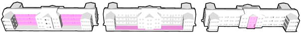 | ||||
| Influencing Factors | Sum of Squares | Degree of Freedom | Mean Square | Test Statistic F | Significance p |
|---|---|---|---|---|---|
| Corridor | 0.001 | 2 | 0.000 | 0.245 | 0.720 |
| Courtyard | 0.005 | 2 | 0.002 | 2.213 | 0.171 |
| Foyer | 0.003 | 2 | 0.001 | 1.118 | 0.431 |
| Influencing Factors | Sum of Squares | Degree of Freedom | Mean Square | Test Statistic F | Significance p |
|---|---|---|---|---|---|
| Corridor | 0.169 | 2 | 0.084 | 0.203 | 0.822 |
| Courtyard | 1.849 | 2 | 0.924 | 6.820 | 0.029 |
| Foyer | 0.629 | 2 | 0.314 | 0.928 | 0.447 |
| Number | How the Buffer Space Is Combined | Average Indoor Air Speed (m/s) | Average Indoor Temperature (°C) |
|---|---|---|---|
| 1 | A3B3C1 | 0.05 | 28.5 |
| 2 | A1B2C3 | 0.1 | 27.6 |
| 3 | A3B1C3 | 0.01 | 27.1 |
| 4 | A1B3C2 | 0.02 | 28.3 |
| 5 | A2B3C3 | 0.01 | 28.3 |
| 6 | A3B2C2 | 0.12 | 27.1 |
| 7 | A2B2C1 | 0.02 | 28.0 |
| 8 | A2B1C1 | 0.01 | 27.0 |
| 9 | A1B1C1 | 0.02 | 27.8 |
| Item | Level | Corridor (A) | Courtyard (B) | Foyer (C) |
|---|---|---|---|---|
| K avg | 1 | 0.04 | 0.01 | 0.02 |
| 2 | 0.01 | 0.08 | 0.07 | |
| 3 | 0.06 | 0.02 | 0.04 | |
| Optimal level | 3 | 2 | 2 | |
| Range | 0.05 | 0.07 | 0.04 | |
| Sort of factors | B > A > C | |||
| Item | Level | Corridor (A) | Courtyard (B) | Foyer (C) |
|---|---|---|---|---|
| K avg | 1 | 27.9 | 27.3 | 27.82 |
| 2 | 27.77 | 27.57 | 27.7 | |
| 3 | 27.57 | 28.37 | 27.67 | |
| Optimal level | 1 | 3 | 1 | |
| Range | 0.33 | 1.07 | 0.16 | |
| Sort of factors | B > A > C | |||
| Influencing Factors | Sum of Squares | Degree of Freedom | Mean Square | Test Statistic F | Significance p |
|---|---|---|---|---|---|
| Corridor | 0.003 | 2 | 0.002 | 1.405 | 0.416 |
| Courtyard | 0.007 | 2 | 0.004 | 3.027 | 0.248 |
| Foyer | 0.001 | 2 | 0.002 | 0.243 | 0.804 |
| Influencing Factors | Sum of Squares | Degree of Freedom | Mean Square | Test Statistic F | Significance p |
|---|---|---|---|---|---|
| Corridor | 0.169 | 2 | 0.084 | 10.857 | 0.084 |
| Courtyard | 1.849 | 2 | 0.924 | 118.857 | 0.008 |
| Foyer | 0.629 | 2 | 0.314 | 40.429 | 0.024 |
| Dependent Variable: Room Temperature LSD | Mean Difference (I − J) | 95% Confidence Interval | ||||
|---|---|---|---|---|---|---|
| (I) Corridor | (J) Corridor | Standard Error | Significance | Lower Limit | Upper Limit | |
| 16 × 2 × 3.3 | 16 × 2.5 × 3.6 | 0.133 | 0.0720 | 0.205 | −0.176 | 0.443 |
| 16 × 3 × 3.9 | 0.333 * | 0.0720 | 0.044 | 0.024 | 0.643 | |
| 16 × 2.5 × 3.6 | 16 × 2 × 3.3 | −0.133 | 0.0720 | 0.205 | −0.443 | 0.176 |
| 16 × 3 × 3.9 | 0.200 | 0.0720 | 0.109 | −0.110 | 0.510 | |
| 16 × 3 × 3.9 | 16 × 2 × 3.3 | −0.333 * | 0.0720 | 0.044 | −0.643 | −0.024 |
| 16 × 2.5 × 3.6 | −0.200 | 0.0720 | 0.109 | −0.510 | 0.110 | |
| Dependent Variable: Room Temperature LSD | Mean Difference (I − J) | 95% Confidence Interval | ||||
|---|---|---|---|---|---|---|
| (I) Courtyard | (J) Courtyard | Standard Error | Significance | Lower Limit | Upper Limit | |
| 16 × 8 | 16 × 10 | −0.267 | 0.0720 | 0.066 | −0.576 | 0.043 |
| 16 × 12 | −1.067 * | 0.0720 | 0.005 | −1.376 | −0.757 | |
| 16 × 10 | 16 × 8 | 0.267 | 0.0720 | 0.066 | −0.043 | 0.576 |
| 16 × 12 | −0.800 * | 0.0720 | 0.008 | −1.110 | −0.490 | |
| 16 × 12 | 16 × 8 | 1.067 * | 0.0720 | 0.005 | 0.757 | 1.376 |
| 16 × 10 | 0.800 * | 0.0720 | 0.490 | 0.490 | 1.110 | |
| Dependent Variable: Room Temperature LSD | Mean Difference (I − J) | 95% Confidence Interval | ||||
|---|---|---|---|---|---|---|
| (I) Foyer | (J) Foyer | Standard Error | Significance | Lower Limit | Upper Limit | |
| 7.2 × 6 × 3.3 | 7.2 × 8 × 3.6 | 0.633 * | 0.0720 | 0.013 | 0.324 | 0.943 |
| 7.2 × 10 × 3.9 | 0.433 * | 0.0720 | 0.027 | 0.124 | 0.743 | |
| 7.2 × 8 × 3.6 | 7.2 × 6 × 3.3 | −0.633 * | 0.0720 | 0.013 | −0.943 | −0.324 |
| 7.2 × 10 × 3.9 | −0.200 | 0.0720 | 0.109 | −1.510 | 0.110 | |
| 7.2 × 10 × 3.9 | 7.2 × 6 × 3.3 | −0.433 * | 0.0720 | 0.027 | −0.743 | −0.124 |
| 7.2 × 8 × 3.6 | 0.200 | 0.0720 | 0.109 | −0.110 | 0.510 | |
Disclaimer/Publisher’s Note: The statements, opinions and data contained in all publications are solely those of the individual author(s) and contributor(s) and not of MDPI and/or the editor(s). MDPI and/or the editor(s) disclaim responsibility for any injury to people or property resulting from any ideas, methods, instructions or products referred to in the content. |
© 2024 by the authors. Licensee MDPI, Basel, Switzerland. This article is an open access article distributed under the terms and conditions of the Creative Commons Attribution (CC BY) license (https://creativecommons.org/licenses/by/4.0/).
Share and Cite
Gan, S.; Chen, W.; Feng, J. Case Study of Space Optimization Simulation of Existing Office Buildings Based on Thermal Buffer Effect. Buildings 2024, 14, 1611. https://doi.org/10.3390/buildings14061611
Gan S, Chen W, Feng J. Case Study of Space Optimization Simulation of Existing Office Buildings Based on Thermal Buffer Effect. Buildings. 2024; 14(6):1611. https://doi.org/10.3390/buildings14061611
Chicago/Turabian StyleGan, Shenqi, Wenxiang Chen, and Jiawang Feng. 2024. "Case Study of Space Optimization Simulation of Existing Office Buildings Based on Thermal Buffer Effect" Buildings 14, no. 6: 1611. https://doi.org/10.3390/buildings14061611
APA StyleGan, S., Chen, W., & Feng, J. (2024). Case Study of Space Optimization Simulation of Existing Office Buildings Based on Thermal Buffer Effect. Buildings, 14(6), 1611. https://doi.org/10.3390/buildings14061611