
Cyclic Void Growth Model Parameter Calibration of Q460D Steel and ER55-G Welds after Exposure to High Temperatures
Abstract
:1. Introduction
2. Basic Theory of Micromechanical Fracture Model CVGM
3. Cyclic Experiments on Notched Round Bar Specimens Following Exposure to High Temperatures Followed by Natural Cooling
3.1. Coupon Test Results
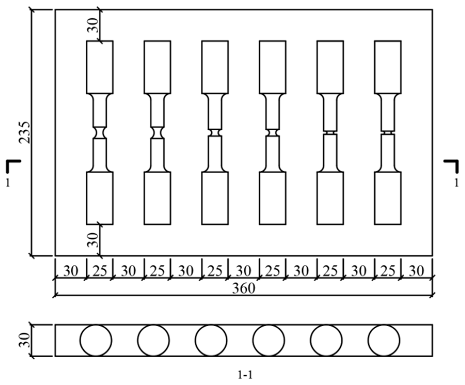
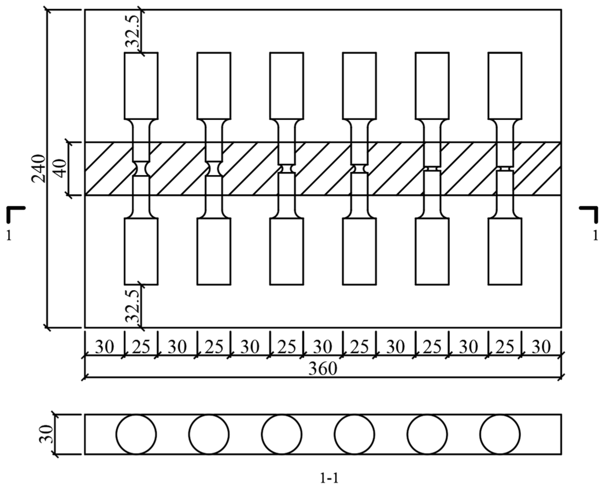
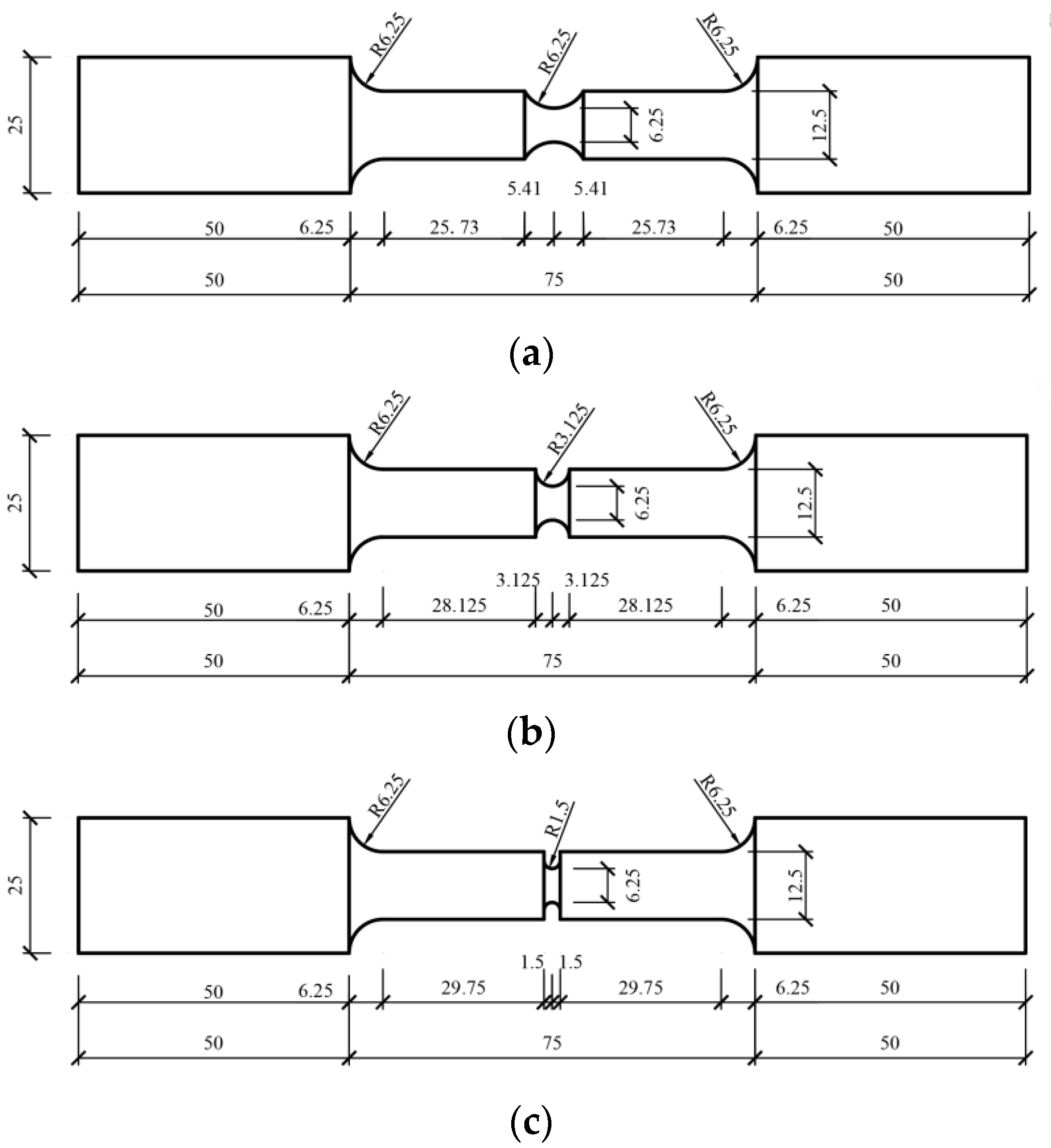
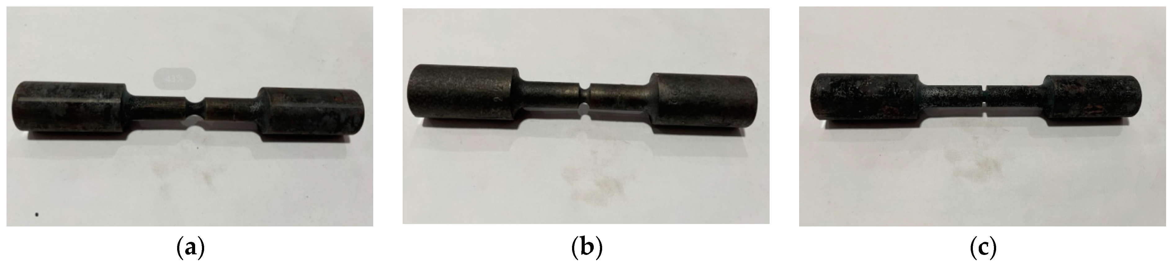
3.2. Design and Manufacture of Notched Round BAR Cyclic Test Specimens
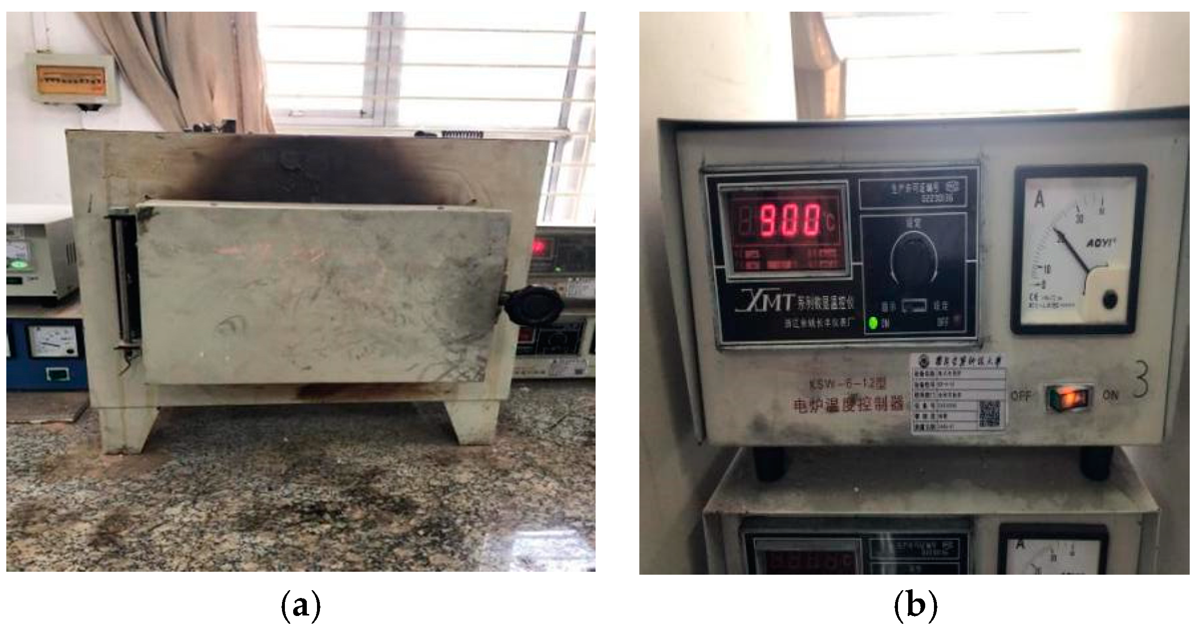
3.3. Treatment of Thermal Exposure and Subsequent Natural Cooling of Notched Round Bar Specimens
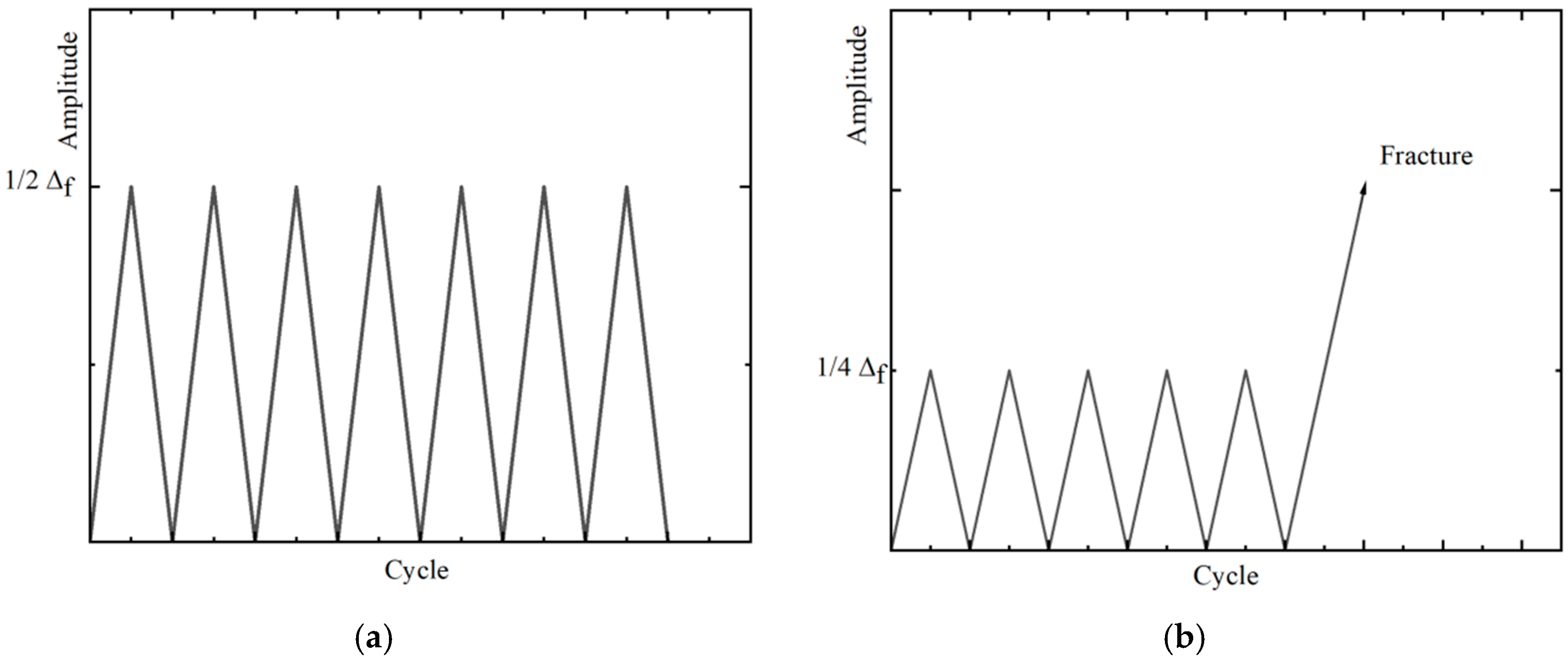
3.4. ULCF Loading Test on Notched Round Bar Specimen Following Exposure to High Temperatures and Subsequent Natural Cooling
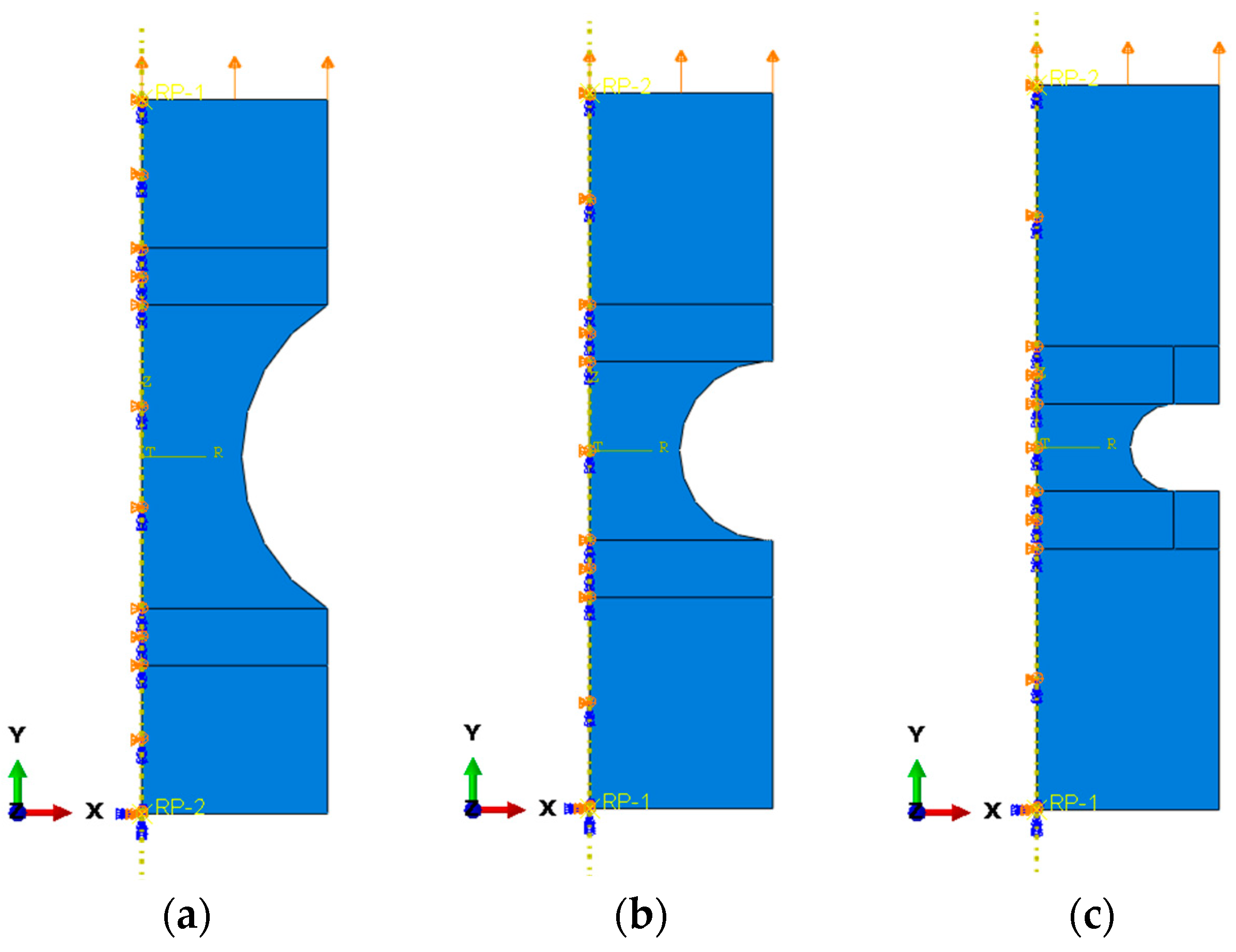
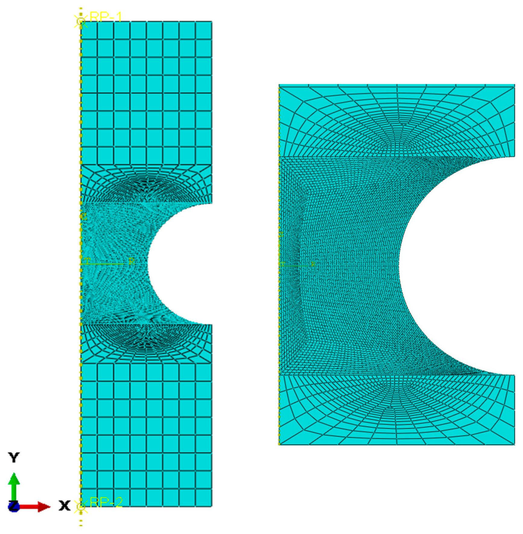
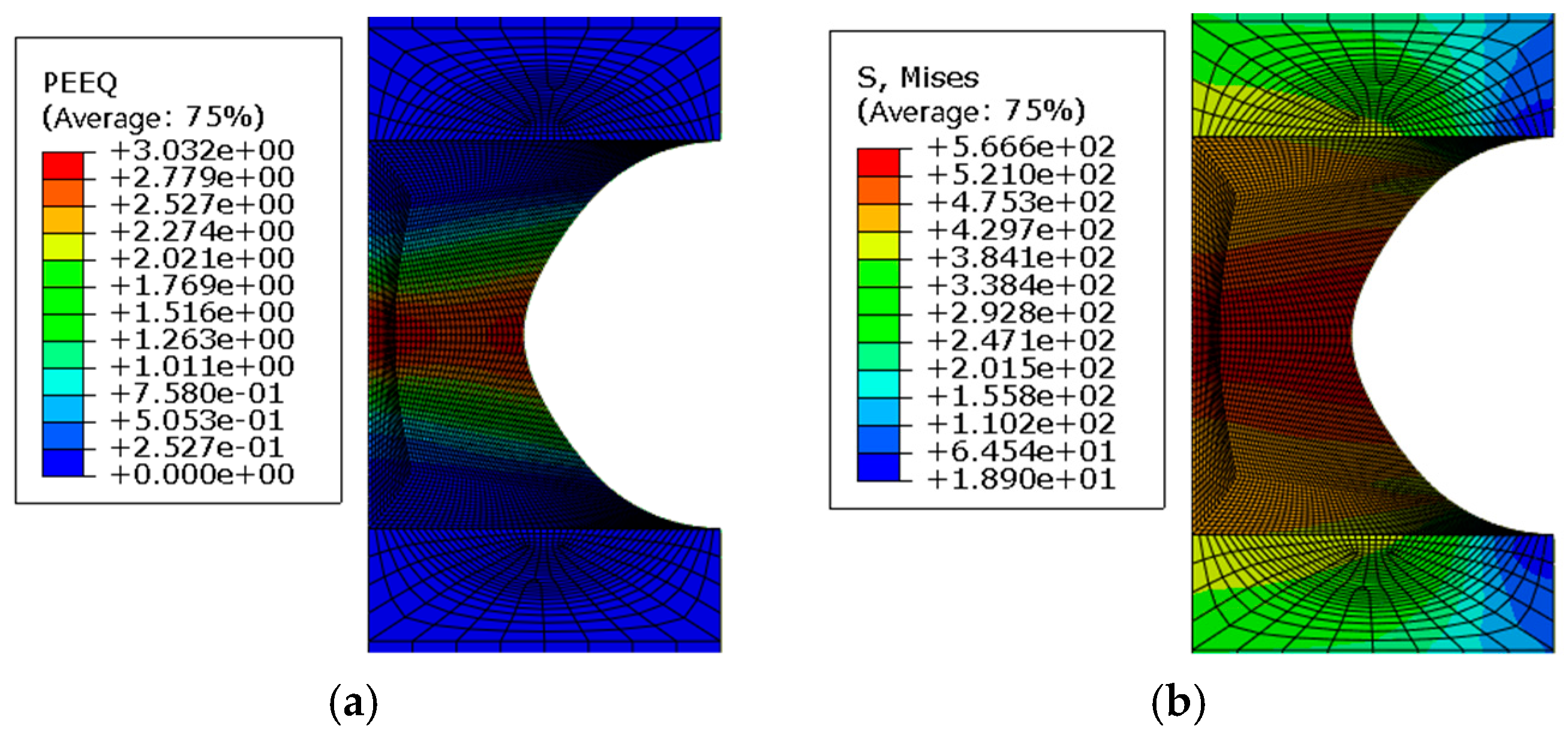
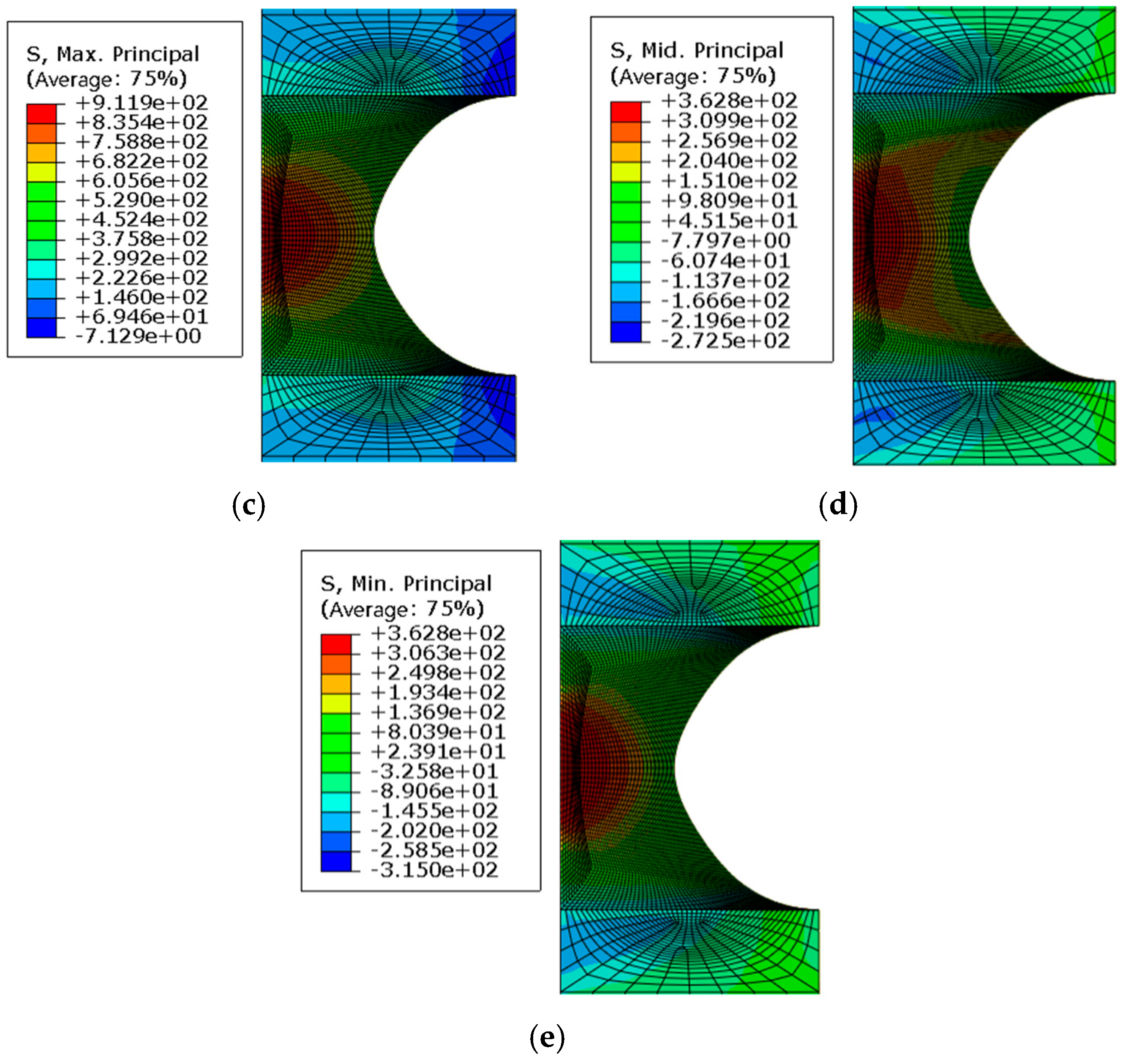
4. FEA of Notched Round Bar Specimen Following Exposure to High Temperatures and Subsequent Natural Cooling
5. Calibration of CVGM Parameters
6. Fracture Prediction
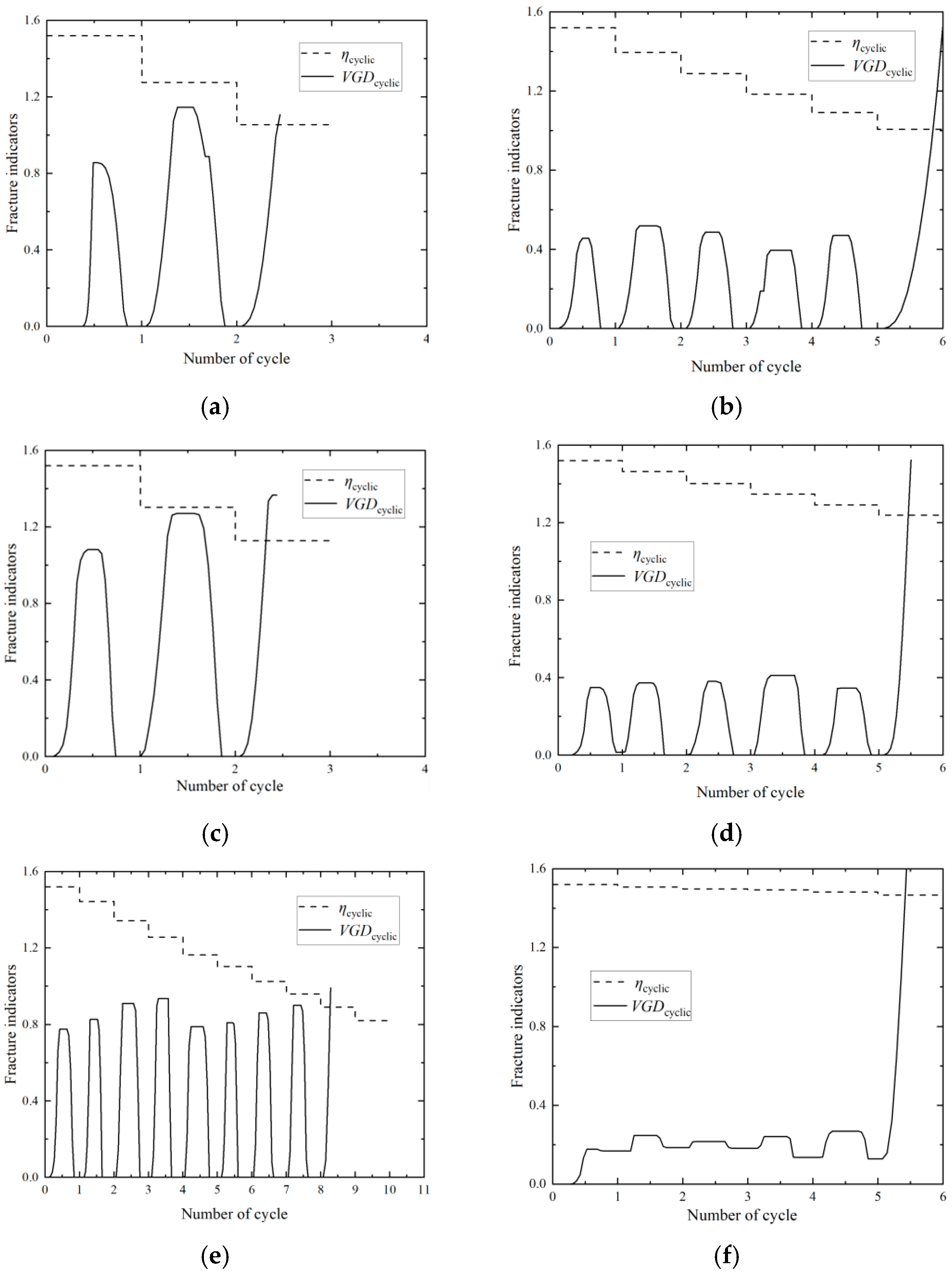
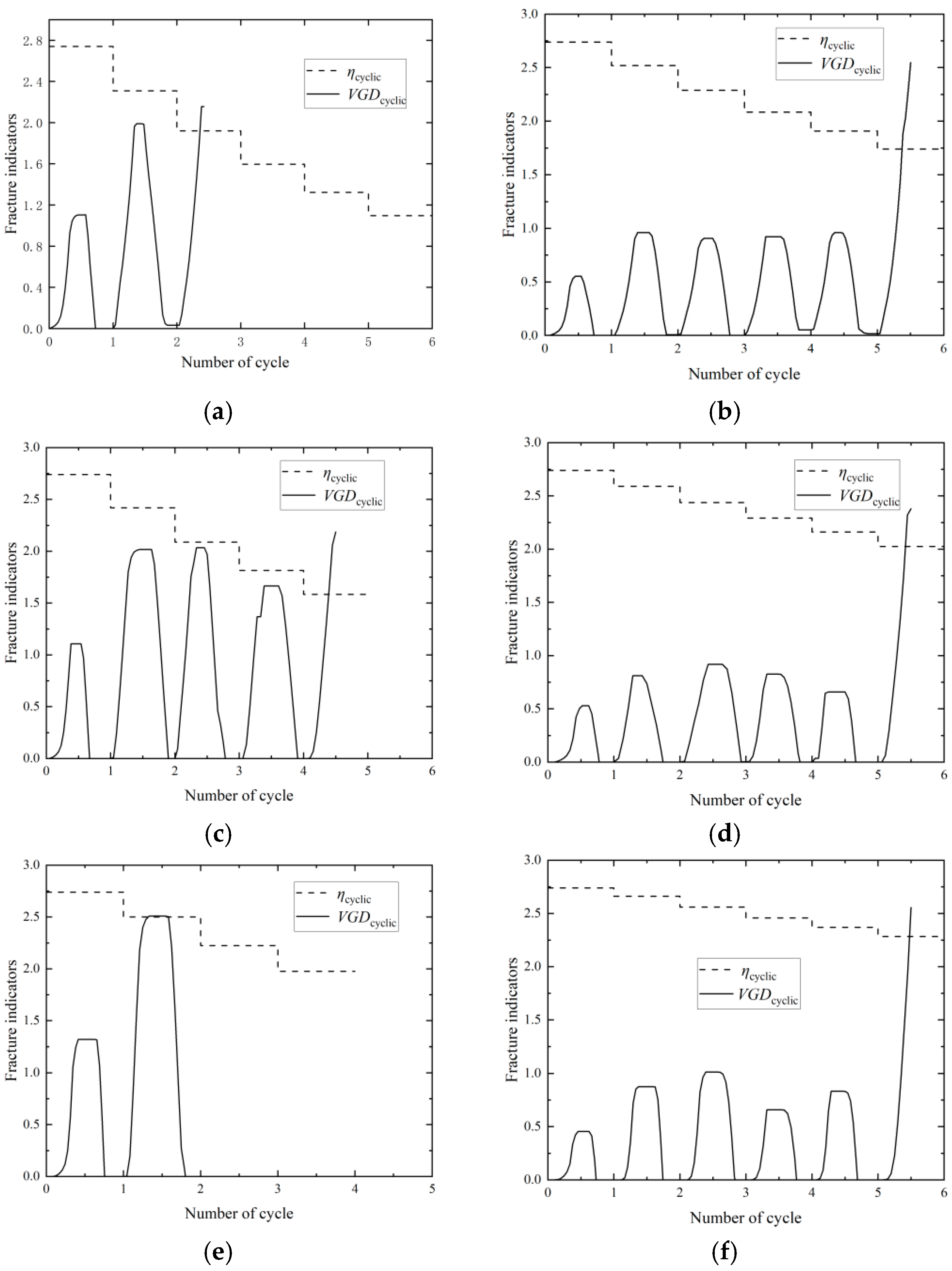
6.1. CVGM Prediction Principle
6.2. CVGM Prediction Results
7. Conclusions
- (1)
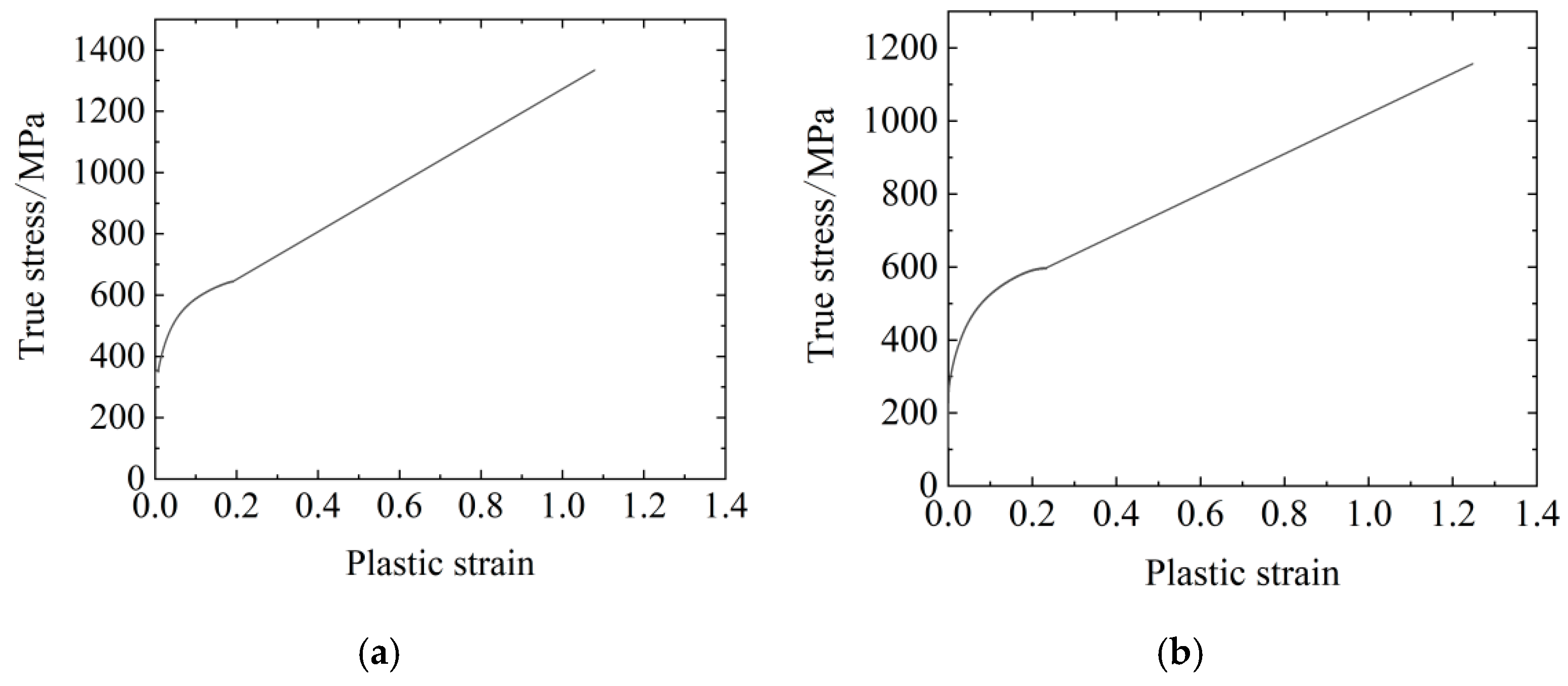
- The true stresses of Q460D steel at the yield moment and the fracture moment were higher while the plastic strain of Q460D steel was lower compared with those of ER55-G welds.
- (2)
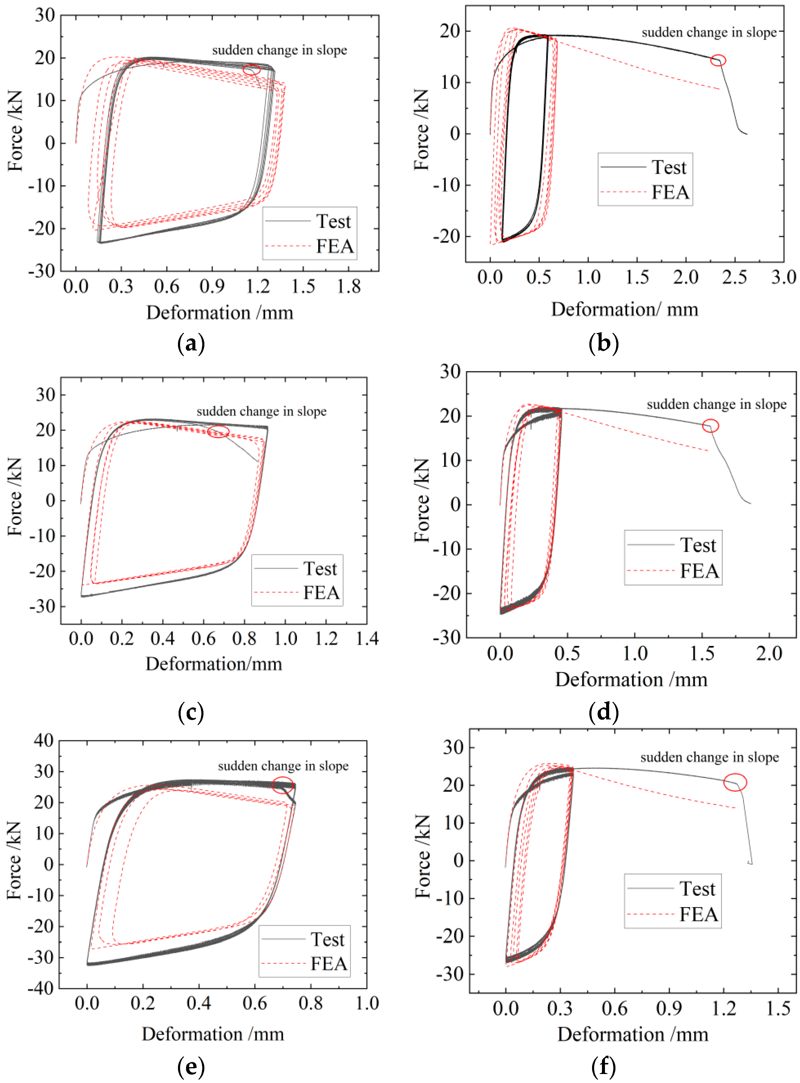
- The force–deformation curves from the FEA and the tests displayed good agreement for most of the notched round bar specimens, while the deviation of the FEA curve with the test curve of some notched round bar specimens was relatively large. The reason for this may be that the parameters Q∞ and b used in the FEA were obtained from a trial process, and occasionality always occurs in this test.
- (3)
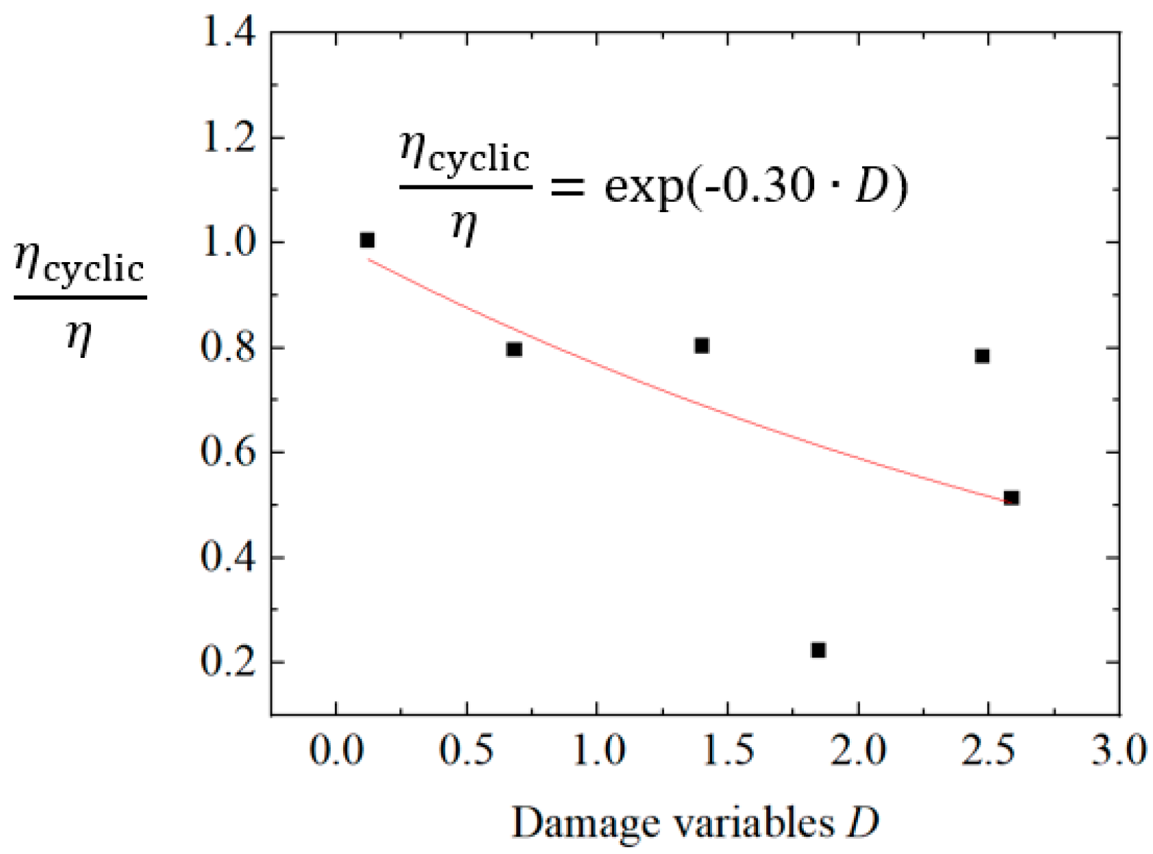
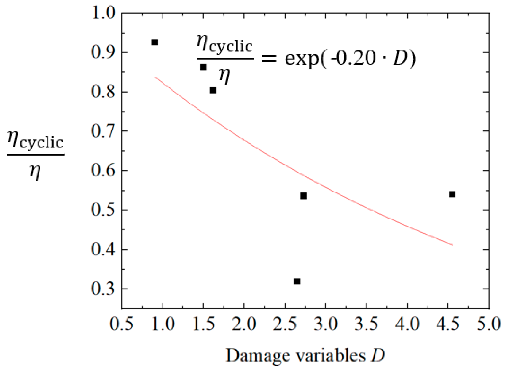
- The damage degradation parameter of the CVGM of Q460D steel and ER55-G welds following exposure to 900 °C and subsequent natural cooling under ULCF loading was 0.30 and 0.20, respectively. The value of the characteristic length parameter of the CVGM of Q460D steel and ER55-G welds post-high-temperature-treatment at 900 °C and natural cooling under ULCF loading was determined to be 0.162 mm and 0.124 mm, respectively.
- (4)
- The fracture index decreased with the increase in the number of cycles.
- (5)
- The calibrated CVGM was capable of accurately predicting the initiation of ductile fracture in Q460D steel and ER55-G welds following exposure to 900 °C and subsequent natural cooling under ULCF loading. The deviations of the predicted results of specimens QZ-W-3, QZ-W-5, and EZ-W-1 were relatively large. The reasons for this may be that the points determined by the damage ratio and the damage variable D of these specimens were relatively far from the fitted curve, the mean values of for Q460D steel and ER55-G welds following exposure to 900 °C and subsequent natural cooling mentioned in ref. [4] were used in the calibration process of , there were deviations of the values of , and there may have been test occasionality.
Author Contributions
Funding
Data Availability Statement
Conflicts of Interest
References
- Bjorhovde, R. Development and use of high performance steel. J. Constr. Steel Res. 2004, 60, 393–400. [Google Scholar] [CrossRef]
- Ke, K.; Chen, Y.; Zhou, X.; Yam, M.C.; Hu, S. Experimental and numerical study of a brace-type hybrid damper with steel slit plates enhanced by friction mechanism. Thin-Walled Struct. 2023, 182, 110249. [Google Scholar] [CrossRef]
- Zhou, X.; Tan, Y.; Ke, K.; Yam, M.C.; Zhang, H.; Xu, J. An experimental and numerical study of brace-type long double C-section steel slit dampers. J. Build. Eng. 2023, 64, 105555. [Google Scholar] [CrossRef]
- Liao, F.; Liu, Y.; Wang, W.; Lu, Z.; Li, X. Fracture performance study on Q460D steel and ER55-G welds after high temperature. J. Constr. Steel Res. 2023, 206, 107888. [Google Scholar] [CrossRef]
- Chiew, S.P.; Zhao, M.S.; Lee, C.K. Mechanical properties of heat-treated high strength steel under fire/post-fire conditions. J. Constr. Steel Res. 2014, 98, 12–19. [Google Scholar] [CrossRef]
- Heidarpour, A.; Tofts, N.S.; Korayem, A.H.; Zhao, X.L.; Hutchinson, C.R. Mechanical properties of very high strength steel at elevated temperatures. Fire Saf. J. 2014, 64, 27–35. [Google Scholar] [CrossRef]
- Wang, W.Y.; Li, G.Q. Research progress on fire resistance design theory of high strength steel structures. Ind. Constr. 2016, 46, 61–67.9. (In Chinese) [Google Scholar]
- Wang, K. Experimental Study on Mechanical Properties of High-Strength Q690 Steel at Elevated Temperatures; Chongqing University: Chongqing, China, 2016. (In Chinese) [Google Scholar]
- Abuhishmeh, K.; Jalali, H.H.; Ebrahimi, M.; Soltanianfard, M.A.; Correa, C.O.; Cornejo, J.S. Behavior of high strength reinforcing steel rebars after high temperature exposure: Tensile properties and bond behavior using pull-out and end beam tests. Eng. Struct. 2024, 305, 117730. [Google Scholar] [CrossRef]
- Yamaguchi, T.; Ozaki, F. Tensile strengths of super high-strength steel strand wire ropes and wire rope open swaged socket connections at fire and post fire. J. Struct. Fire 2024, 15, 50–75. [Google Scholar] [CrossRef]
- Pandey, M.; Young, B. Cold-formed high strength steel CHS-to-RHS T- and X-joints: Performance and design after fire exposures. Thin-Walled Struct. 2023, 189, 110793. [Google Scholar] [CrossRef]
- Pandey, M.; Young, B. Post-fire behaviour of cold-formed high strength steel tubular T- and X-joints. J. Constr. Steel Res. 2021, 186, 106859. [Google Scholar] [CrossRef]
- Zhuang, Z.; Jiang, Z.P. Engineering Fractures and Damage; China Machine Press: Beijing, China, 2004. [Google Scholar]
- Kanvinde, A.M.; Deierlein, G.G. Void growth model and stress modified critical strain model to predict ductile fracture in structural steels. J. Struct. Eng. ASCE 2006, 132, 1907–1918. [Google Scholar] [CrossRef]
- Rice, J.R.; Tracey, D.M. On the ductile enlargement of voids in triaxial stress fields. J. Mech. Phys. Solids 1969, 17, 201–217. [Google Scholar] [CrossRef]
- Hancock, J.W.; Mackenzie, A.C. On the mechanics of ductile failure in high-strength steel subjected to multi-axial stress states. J. Mech. Phys. Solids 1976, 24, 147–169. [Google Scholar] [CrossRef]
- Kanvinde, A.M.; Deierlein, G.G. Micromechanical Simulation of Earthquake-Induced Fracture in Steel Structures; Stanford University: Stanford, CA, USA, 2004. [Google Scholar]
- Kanvinde, A.M.; Deierlein, G.G. Prediction of Ductile Fracture in Steel Moment Connections During Earthquakes Using Micromechanical Fracture Models. In Proceedings of the 13th World Conference on Earthquake Engineering, Vancouver, BC, Canada, 1–6 August 2004; Volume 297. [Google Scholar]
- Kanvinde, A.M.; Deierlein, G.G. Finite-element simulation of ductile fracture in reduced section pull-plates using micromechanics-based fracture models. J. Struct. Engineering. 2007, 133, 656–664. [Google Scholar] [CrossRef]
- Roufegarinejad, A.; Tremblay, R. Finite element modeling of the inelastic cyclic response and fracture life of square tubular steel bracing members subjected to seismic inelastic loading. In Behavior of Steel Structures in Seismic Areas (STESSA 2012); CRC Press: Boca Raton, FL, USA, 2012; pp. 97–103. [Google Scholar]
- Siriwardane, S.; Ratnayake, R.M.C. A Simple criterion to predict fracture of offshore steel structures in extremely-low cycle fatigue region. In Proceedings of the International Conference on Offshore Mechanics and Arctic Engineering, Rio de Janeiro, Brazil, 1–6 July 2012; pp. 211–218. [Google Scholar]
- Wang, Y.; Zhou, H.; Shi, Y.; Xiong, J. Fracture prediction of welded steel connections using traditional fracture mechanics and calibrated micromechanics based models. Int. J. Steel Struct. 2011, 11, 351–366. [Google Scholar] [CrossRef]
- Liao, F.F.; Wang, W.; Chen, Y.Y. Parameter calibrations and application of micromechanical fracture models of structural steels. Struct. Eng. Mech. 2012, 42, 153–174. [Google Scholar] [CrossRef]
- Liao, F.F.; Wang, R.Z.; Li, W.C.; Zhou, T.H. Study on micro mechanism-based ductile fracture criteria for Q460 steel. J. Xi’an Univ. Archit. Technol. (Nat. Sci. Ed.) 2016, 48, 535–543+550. (In Chinese) [Google Scholar]
- Liao, F.; Wang, M.; Tu, L.; Wang, J.; Lu, L. Micromechanical fracture model parameter influencing factor study of structural steels and welding materials. Constr. Build. Mater. 2019, 215, 898–917. [Google Scholar] [CrossRef]
- Liao, F.F.; Wang, W.; Chen, Y.Y. Extremely low cycle fatigue fracture prediction of steel connections under cyclic loading. J. Tongji Univ. (Nat. Sci.) 2014, 42, 539–546+617. (In Chinese) [Google Scholar]
- Li, K.K. Study on Extremelylow Cycle Fatigue Fracture Performance of Q460 High-Strength Steel Welded Beam-Column Connections with Different Welding Hole Structures; Chang’an University: Xi’an, China, 2020. (In Chinese) [Google Scholar]
- Yu, Z.W.; Wang, Z.Q.; Shi, Z.F. Experimental research on material properties of new III grade steel bars after fire. J. Build. Struct. 2005, 26, 112–116. (In Chinese) [Google Scholar]
- GB 50661-2011; Code for Welding of Steel Structures. China Building Industry Press: Beijing, China, 2011. (In Chinese)
- Lemaitre, J.; Chaboche, J.L. Mechanics of Solid Materials. Master’s Thesis, Cambridge University Press, Cambridge, UK, 1990. [Google Scholar]


| Material | Specimen Number | (MPa) | (MPa) | (MPa) |
|---|---|---|---|---|
| Q460D steel (room temperature) | QD-1 | 419 | 540 | 200,703 |
| QD-2 | 478 | 618 | 200,191 | |
| QD-3 | 460 | 612 | 202,848 | |
| Mean value | 452 | 590 | 201,247 | |
| Q460D steel (following exposure to 900 °C and subsequent natural cooling) | QZD-1 | 351 | 539 | 183,341 |
| QZD-2 | 352 | 545 | 181,774 | |
| QZD-3 | 352 | 538 | 178,606 | |
| Mean value | 352 | 541 | 181,240 | |
| ER55-G welds (room temperature) | ED-1 | 516 | 621 | 209,104 |
| ED-2 | 498 | 616 | 204,415 | |
| ED-3 | 509 | 606 | 201,321 | |
| Mean value | 508 | 614 | 204,947 | |
| ER55-G welds (following exposure to 900 °C and subsequent natural cooling) | EZD-1 | 275 | 511 | 198,462 |
| EZD-2 | 281 | 487 | 199,919 | |
| EZD-3 | 273 | 487 | 185,750 | |
| Mean value | 276 | 495 | 194,710 |
| Q460D steel (following exposure to 900 °C and subsequent natural cooling) | Plastic strain | 0.000 | 0.0001 | 0.0005 | 0.001 | 0.004 | 0.008 | 0.016 | 0.032 |
| True stress (MPa) | 302 | 343 | 350 | 351 | 354 | 355 | 404 | 471 | |
| Plastic strain | 0.049 | 0.065 | 0.081 | 0.099 | 0.131 | 0.164 | 0.192 | 1.079 | |
| True stress (MPa) | 516 | 546 | 566 | 588 | 613 | 633 | 645 | 1334 | |
| ER55-G welds (following exposure to 900 °C and subsequent natural cooling) | Plastic strain | 0.000 | 0.0001 | 0.0005 | 0.001 | 0.0014 | 0.004 | 0.008 | 0.018 |
| True stress (MPa) | 107 | 166 | 228 | 255 | 264 | 289 | 315 | 361 | |
| Plastic strain | 0.036 | 0.049 | 0.068 | 0.088 | 0.131 | 0.179 | 0.233 | 1.248 | |
| True stress (MPa) | 419 | 452 | 484 | 511 | 551 | 582 | 598 | 1157 |
| Material | Specimen Number | Notch Radius | Diameter of Gauge Length Part | Length of Clamping Part | Diameter at the Notch | Loading Amplitude |
|---|---|---|---|---|---|---|
| R (mm) | (mm) | (mm) | (mm) | (mm) | ||
| Q460D steel | QZ-W-1 | 6.25 | 12.80 | 50.23 | 6.88 | 0.97 |
| QZ-W-2 | 12.80 | 50.22 | 6.76 | 0.485 (5) | ||
| QZ-W-3 | 3.125 | 12.86 | 50.26 | 6.32 | 0.655 | |
| QZ-W-4 | 12.70 | 50.23 | 7.28 | 0.3275 (5) | ||
| QZ-W-5 | 1.5 | 12.64 | 50.19 | 6.48 | 0.425 | |
| QZ-W-6 | 12.76 | 50.29 | 6.76 | 0.2125 (5) | ||
| ER55-G welds | EZ-W-1 | 6.25 | 12.62 | 49.22 | 6.38 | 1.385 |
| EZ-W-2 | 12.60 | 49.27 | 6.38 | 0.6925 (5) | ||
| EZ-W-3 | 3.125 | 12.58 | 49.15 | 6.38 | 0.915 | |
| EZ-W-4 | 12.58 | 49.32 | 6.38 | 0.4575 (5) | ||
| EZ-W-5 | 1.5 | 12.68 | 49.54 | 6.34 | 0.745 | |
| EZ-W-6 | 12.58 | 49.58 | 6.36 | 0.3725 (5) |
| Material | Equivalent Stress (MPa) | b | |
|---|---|---|---|
| Q460D steel | 302 | 180 | 145 |
| ER55-G welds | 107 | 205 | 80 |
| Specimen Number | Fracture Load (kN) | Fracture Displacement (mm) | Number of Cycles | |
|---|---|---|---|---|
| QZ-W-1 | Test | 18.13 | 0.30 | 4 |
| Prediction | 23.49 | 0.86 | 3 | |
| Deviation | 29.56% | 186.67% | −1 | |
| QZ-W-2 | Test | 17.02 | 1.66 | 6 |
| Prediction | 22.75 | 1.21 | 6 | |
| Deviation | 33.67% | −27.11% | 0 | |
| QZ-W-3 | Test | 20.95 | 0.23 | 6 |
| Prediction | 21.61 | 0.64 | 3 | |
| Deviation | 3.15% | 178.26% | −3 | |
| QZ-W-4 | Test | 20.09 | 1.05 | 6 |
| Prediction | 29.16 | 1.06 | 6 | |
| Deviation | 45.15% | 0.95% | 0 | |
| QZ-W-5 | Test | 18.55 | 0.36 | 12 |
| Prediction | 25.30 | 0.18 | 8 | |
| Deviation | 36.39% | −50% | −4 | |
| QZ-W-6 | Test | 22.07 | 0.95 | 6 |
| Prediction | 28.46 | 0.66 | 6 | |
| Deviation | 28.95% | −30.53% | 0 | |
| EZ-W-1 | Test | 17.13 | 1.16 | 6 |
| Prediction | 16.81 | 1.31 | 3 | |
| Deviation | −1.87% | 12.93% | −3 | |
| EZ-W-2 | Test | 14.19 | 2.35 | 6 |
| Prediction | 17.28 | 1.65 | 6 | |
| Deviation | 21.78% | −29.79% | 0 | |
| EZ-W-3 | Test | 19.64 | 0.67 | 5 |
| Prediction | 17.80 | 0.57 | 5 | |
| Deviation | −9.37% | −14.93% | 0 | |
| EZ-W-4 | Test | 17.62 | 1.56 | 6 |
| Prediction | 18.66 | 1.51 | 6 | |
| Deviation | 5.90% | −3.21% | 0 | |
| EZ-W-5 | Test | 24.53 | 0.70 | 4 |
| Prediction | 21.72 | 0.73 | 2 | |
| Deviation | −11.46% | 4.29% | −2 | |
| EZ-W-6 | Test | 20.38 | 1.27 | 6 |
| Prediction | 21.41 | 0.67 | 6 | |
| Deviation | 5.05% | −47.24% | 0 |
Disclaimer/Publisher’s Note: The statements, opinions and data contained in all publications are solely those of the individual author(s) and contributor(s) and not of MDPI and/or the editor(s). MDPI and/or the editor(s) disclaim responsibility for any injury to people or property resulting from any ideas, methods, instructions or products referred to in the content. |
© 2024 by the authors. Licensee MDPI, Basel, Switzerland. This article is an open access article distributed under the terms and conditions of the Creative Commons Attribution (CC BY) license (https://creativecommons.org/licenses/by/4.0/).
Share and Cite
Liao, F.; Yang, Z.; Wang, J.; Fang, P.; Liu, X.; Li, X. Cyclic Void Growth Model Parameter Calibration of Q460D Steel and ER55-G Welds after Exposure to High Temperatures. Buildings 2024, 14, 1622. https://doi.org/10.3390/buildings14061622
Liao F, Yang Z, Wang J, Fang P, Liu X, Li X. Cyclic Void Growth Model Parameter Calibration of Q460D Steel and ER55-G Welds after Exposure to High Temperatures. Buildings. 2024; 14(6):1622. https://doi.org/10.3390/buildings14061622
Chicago/Turabian StyleLiao, Fangfang, Zhiyan Yang, Jinhu Wang, Pujing Fang, Xian Liu, and Xiaohong Li. 2024. "Cyclic Void Growth Model Parameter Calibration of Q460D Steel and ER55-G Welds after Exposure to High Temperatures" Buildings 14, no. 6: 1622. https://doi.org/10.3390/buildings14061622