Exploring Historical Perspectives in Building Hygrothermal Models: A Comprehensive Review

Abstract

The necessity of understanding and simulating hydrological phenomena as well as their interactions and the effect of anthropogenic and climate conditions on the ecosystem have encouraged researchers for years to investigate the moisture transfer in soil. Considering the moisture transfer as an isothermal phenomenon might cause a wrong estimation due to the non-isothermal nature of the moisture movement in porous media. Hygrothermal (coupled heat and moisture transfer) models are quite diverse and are the engine of the various hygrothermal software tools used to analyze the heat and moisture in building envelopes, drying technologies, and many other applications. This paper is a literature survey conducted to provide an overview on the classical hygrothermal models to address the historical perspectives on these models. First, it investigated, from a historical point of view, the challenges behind the development of hygrothermal models as unsaturated flow theories, beginning with Buckingham theory. The non-isothermal nature of moisture was the starting point for researchers to deal with new challenges during mathematical modeling and experimental analysis. In general, the theory of coupled heat and moisture transfer first developed by J.R. Philip and De Vries and the authors in the mid-1950s inspired the novel hygrothermal models, including Sophocleous and Milly’s model, Rode’s model, Künzel’s model, and Grunewal’s model. In a parallel of hygrothermal model developments, the models of Whitaker and Luikov can also be classified as hygrothermal models; they were mostly applied in modeling the phenomenon of drying. The study highlights the application of hygrothermal models in building physics and gathered a summary of international efforts such as Annex 24, Annex 41, and the HAMSTAD project and advancements performed from the classical dew point or steady-state Glaser method. Moreover, this study emphasizes the advantages of the standard of EN 15026 and limitations of the Glaser method. To sum up, hygrothermal models are still under development based on various assumptions of moisture driving potentials and transfer coefficients.

1. Introduction

The concept of moisture encompasses both the liquid and vapor states of water. Moisture transfer is governed by a number of mechanisms that account for both liquid and vapor movement [1]. The term “coupled” in studying “coupled heat and moisture transfer”, in fact, refers to considering the temperature effect on moisture flow as well as taking into account the moisture effect when analyzing heat and moisture exchange [2]. In addition, the term hygrothermal refers to the combination of heat and moisture phenomena. The research on hygrothermal or coupled heat and moisture transfer began as a separate field of research during the 1930s. In the mid-1950s, a moisture transfer analysis based on steady-state diffusion was published by Helmut Glaser [3]. In the early 1960s and late 1950s, the first hygrothermal models were published, accounting for vapor and capillary transport, initial state of moisture, latent heat of evaporation, and transient conditions. These developed models were utilized in the building sector to predict moisture conditions in building materials. Buildings are continuously exposed to changes in indoor and outdoor climatic conditions. Constant variations in temperature, moisture, and air pressure have a significant impact on the structural integrity and performance of buildings [4,5]. A number of programming codes have subsequently been developed and commercialized in the construction sector (see [6,7]). A complete hygrothermal model is required to reach precise and optimal parameters in building performance analysis. Figure 1 shows the concept of hygrothermal load in a building envelope affected by precipitation and solar loading.

Nowadays, hygrothermal issues are gaining more attention in porous building materials. The coupled heat and moisture transfer significantly influences the building’s performance in terms of thermal comfort [8], building energy analysis [9], mold growth assessment [10], and moisture-related envelope durability [11]. Recent studies in the hygrothermal field have focused on either laboratory experimentation or modeling. In the field of building energy analysis, Building Energy Simulation (BES) is employed to determine the energy requirements for a structure. The BES approach involves utilizing a single mass model that estimates physical parameters within a single node. The distribution of these parameters remains consistent throughout the designated area, enabling the consideration of long-term dynamic analysis. Following BES research, Indira et al. [12] investigated a building’s energy consumption using CitySim software with a mesoscale climate model utilizing a city-level climate modeling and building energy simulation. Instead of using conventional methods which consider reference buildings, the city of Seoul studied how to improve energy consumption. Carolina et al. [13] analyzed a public educational building on site and also modeled its energy usage using TRNSYS software version 18. They collected the indoor temperature and humidity on the site of the building and took into account the billing information of natural gas and electric bills. In another study conducted by Kalair et al. [14], TRNSYS 18 software was used for thermal comfort analysis in addition to dynamic energy simulation. The annual comfort percentage reflected an increase from 49% to 87.5%, showing a 38.5% increase in thermal demands.

Due to the strong dependency between human well-being, moisture, and mold growth in building envelopes, mold growth becomes a simple criterion in hygrothermal assessment in bio-based or sensitive materials [15]. Naja et al. [16] investigated the hygrothermal condition of nine residential building façades in Nuuk and Sisimiut, Denmark. On-site monitored data were compared against the Delphin model (Delphin 6 software, hygrothermal simulation tool). Hygrothermal data were utilized in free software WUFI (R) mold index VTT for mold growth analysis. Investigating various wall assemblies showed that implementing a wind barrier did not eliminate mold growth risk. Boardman et al. [17] developed a novel mold growth model named DR SIM (dose–response simple isopleth for mold) for wood-based building assemblies. DR SIM was optimized by a large database of laboratory growth results obtained from the literature. One of the advantages of this model is its ability to numerically capture the stochastic nature of mold growth using the deterministic algorithm. More data are required to test the DR SIM model in a comparison of more widely used classical models like MRD (Mold Resistance Design) or VTT models [18]. There is a wide availability of hygrothermal models in scientific communities where the moisture-related effects become non-negligible. Long-term hygrothermal assessment of multi-layer building materials or whole building simulations can be very time-consuming, especially during parametric analysis or in finer mesh two-dimensional investigations [19]. Recent references [20,21,22,23] report the extensive time effort of multi-layered hygrothermal simulation in various wall assemblies. Thus, in order to reduce the computational time and lower resource intensity in hygrothermal assessment, the incorporation of Moisture Reference Years (MRY) has evolved into a standard practice guideline. Generally, trusted MRY data are based on a single year that reflects as much as ten consecutive years of long-term moisture-related risk [24].

In the presence of a significant rate of condensation or evaporation of water in a porous material, the phenomena are necessarily coupled and non-isothermal. Consequently, hygrothermal phenomena have never been a simple system involving only a single driving force and flux. There is no doubt that assessing the hygrothermal performance of an entire building can be both time-consuming and expensive. Besides that, there has been a wide range of literature which made an effort to assess the hygrothermal model either by laboratory experimentation or modelling. Gaining insight into hygrothermal phenomena requires modeling, while experiments allow validating some of the steps in modeling, and field experience allows gaining a reliable, well-balanced understanding of hygrothermal facts and figures. However, hygrothermal models are under development and there is no one direct model that suits the moisture transfer in porous media.

This paper guides researchers in understanding the timeline of hygrothermal developments from challenges encountered from the starting point. Challenges still exist behind these models because of the nature of moisture transfer phenomena. It would help users to select suitable hygrothermal models for various applications, from drying phenomena to building physics.

Since the theory of Philip and De Vries on hygrothermal dynamics, published in 1957 [25], many models have been developed on the basis of this theory by considering the interaction of the vapor and liquid phases of water. With all challenges ahead of the theory of Philip and De Vries, many phenomenological definitions of water in soil were known, including Darcy’s law in 1985 and Buckingham’s theory for unsaturated porous media in 1907, dynamic effects of capillarity in soils (Johnson and King in the years of 1878 and 1889), etc. In Section 2, the development of hygrothermal phenomena for non-isothermal flow will be explained, from Buckingham’s theory for unsaturated flow to Philip and De Vries theory. In the Section 3 and Section 4, classical hygrothermal models will be examined in somewhat more detail, including the models of Philip and De Vries, Luikov, Whitaker and Künzel, Rode, and Grunewald, which are the basis of most commercial software in building application fields. In the discussion part (Section 4), a brief review was created on the advantages and disadvantages of various hygrothermal models. To sum up, the methodology followed in this paper is organized into three phases. The first phase entails providing on historical point of view about hygrothermal phenomena and challenges encountered over the years. The second phase comprises a summary of selected classical models based on the various points of view on hygrothermal driving potentials followed by a discussion on advantages and disadvantages of the models. The third phase includes the progression of the Glaser method to transient methods by gathering the international efforts carried out in this domain.

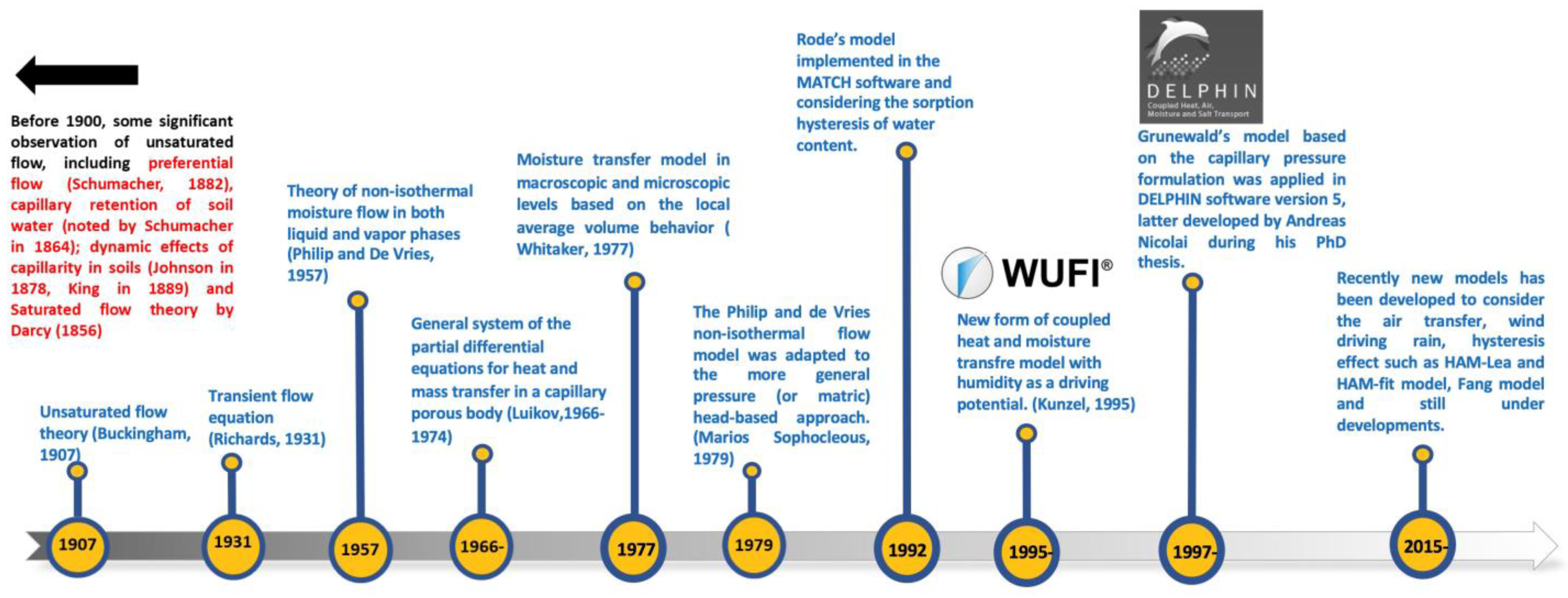
2. A Brief History of Hygrothermal Models

Fredlund and Rahardjo (1993) highlight that classical soil mechanics and geotechnical engineering often assume soil is either completely dry (0% saturation) or fully saturated (100% saturation). According to this view, soil behavior is dictated solely by Terzaghi’s effective stress principle. However, dry and saturated states are merely two extremes of soil conditions. Most soils are unsaturated, with a degree of saturation ranging from 0% to 100% [26]. When water gradually infiltrates soil due to external pressure or capillary action, three zones develop: unsaturated, transient, and saturated (as shown in Figure 2) [27].

Flow through saturated soil was established empirically by Darcy in 1856 and has since then been verified experimentally on numerous occasions [28]. Darcy suggested that the rate of water flow through a soil mass is proportional to the hydraulic head gradient:

$$q_w=-K_s \frac{\partial h_w}{\partial z}$$

(1)

where $q_w$ is the flow rate of water, and $K_s$ and $\frac{\partial h_w}{\partial z}$ denote the saturated coefficient of permeability or saturated hydraulic conductivity and hydraulic head gradient in the z direction, respectively. In unsaturated soil, the coefficient of permeability is significantly affected by changes in both the void ratio and the degree of saturation (or water content) of the soil. Generally, the coefficient of permeability increases as the soil’s void ratio increases. The classical concepts of permeability, such as the Kozeny–Carman model proposed by Kozeny and later modified by Carman [29,30], clearly indicate the dependency of permeability on the void ratio of soil. In 1949, Purcell introduced the first and simplest model, considering a porous medium to be analogous to a bundle of uniform capillary tubes [29,31,32].

Edgar Buckingham’s famous paper in 1907 [33], with the concept of matric potential or capillary pressure, provided the last piece for the puzzle of the unsaturated flow theory. To develop a quantitative framework for unsaturated soil behavior, numerous foundational principles were already recognized. These include the capillary retention of soil water, originally documented by Schumacher in 1864; the dynamic ramifications of capillarity in soil elucidated by Johnson in 1878 and King in 1889; the heat of wetting in soils investigated by Mitscherlich in 1901; the correlation between hygroscopic water and specific surface area, extensively studied by Mitscherlich in 1901 and Rodewald in 1902; the formulation of Darcy’s law for saturated porous media as postulated by Darcy in 1856; and the application of Darcy’s law with potentials and Laplace’s equation, pioneered by Dupuit in 1863 and subsequently advanced by Slichter in 1898. Additionally, Buckingham introduced the concept of “matric potential”, which parallels established physical analogs like electrical potential in Ohm’s law and temperature in Fourier’s theory, representing the energy required to extract water from soil pores. He also mentioned that this potential is not independent of the water content of soil and measured it indirectly with the column of the wet soil equilibrated in a gravitational field. Based on Buckingham’s perceptive theoretical insights, further soil physicists were able to think up a general equation describing both saturated and unsaturated fluid flow in soil [30,34]:

$$q_w=-K\left(\theta \right) \frac{\partial ({\psi }_p+{\psi }_g)}{\partial z}$$

(2)

where $K\left(\theta \right)$is the hydraulic conductivity for both saturated and unsaturated soil. ${\psi }_p, {\psi }_g$are the gradient in the z direction of the total water potential. This equation can be considered as a generalization of Darcy’s Law and is known as the Buckingham–Darcy Law.

Total matric potential, known as soil suction and capillary pressure, is commonly referred to as the free energy state of soil water, which can be quantitively calculated by Kelvin’s equation, as follows:

$${\psi }_p=\frac{\mathfrak{N}T\rho }{v_m}\ln \left(\phi \right)$$

(3)

where $\rho$ and $\phi$ represent the density of water and relative humidity. $\mathfrak{N}$ and $v_m$represent the universal gas constant and molecular mass of water. Later, in 1986, Nielsen stated that the soil total water potential (${\psi }_{total}$) in energy per unit mass can be divided into the following parts [35]:

$${\psi }_{total}={\psi }_p+{\psi }_z+{\psi }_s+{\psi }_e$$

(4)

where ${\psi }_p$ is the pressure potential, ${\psi }_s$ is the solute potential, ${\psi }_e$ is the electrochemical potential, and ${\psi }_z$ is the gravitational potential. The term ${\psi }_p$ is applied to both saturated and unsaturated media. In the unsaturated soil, ${\psi }_p$represents capillary potential, and in saturated soil it denotes the applied pressure. In terms of formulation of moisture transfer in unsaturated soil media, Buckingham’s theory was the basis for a new generation of moisture transfer models. In turn, this attracted other researchers who have been wishing to develop this theory for various potential effects of moisture transport, such as the solute potential or the electric potential consequences [36]. While the complexity of the moisture transfer map continues to be a challenging issue, the methodology of calculating the moisture coefficients of these potential maps remains a challenge. Due to experimental limitations, measuring these coefficients is still challenging. Therefore, some assumptions were made during the calculation of the moisture transfer coefficients.

L. A. Richards, in 1931, represented the transient flow for unsaturated structured media by combining the Buckingham–Darcy Law with continuity equation [37]. Richards was among the first researchers to predict water transport in partially saturated porous media using the differential form of Darcy’s formula. Although the application of Darcy’s model was for flow in saturated porous media, it has been developed for flow in unsaturated media by providing hydraulic conductivity as a function of the water content. Equations (4) and (5) represent the combination of the Richard’s equation and conduction–convection heat equation [36,38]:

$$\frac{\partial \theta }{\partial t}=\nabla \left[K\left({\psi }_p,T\right)· \nabla { \psi }_p\right]$$

(5)

$$C{\rho }_l\frac{\partial T}{\partial t}=\nabla \left(\lambda \nabla T\right)-\nabla \left(c_l q_w(\mathrm{T}-T_0)\right)$$

(6)

where the parameters of $\theta$, T, and $q_w$ refer to volumetric moisture content, temperature, and Darcy flux density, respectively. $T_0$ and $\lambda$ in the energy equation represent the reference temperature and thermal conductivity of the material. The combination of the Richards equation and conduction–convection heat equation as the governing model represents the water and heat transfer in soil. Such a model formulation does not include temperature gradient as a factor in the flux vapor transfer and associated sensible and latent heat fluxes; it may produce undesirable results in unsaturated soils [39]. Another limitation of Richard’s equation in hygrothermal modeling is that it does not include the vapor phase of liquid. This is because of the interaction of the vapor phase and liquid phase in porous materials. The vapor diffusion can follow the kinetic gas theory of Fick’s law under the conditions of mesopores or larger pores for which molecular diffusion could be negligible. But Fick’s law could only represent the vapor diffusion and not liquid diffusion in hygrothermal phenomena.

In Europe, the starting point of heat and moisture transfer models goes back to the first book on drying technology written by Hirsch in 1932. This book was edited and rewritten in 1956–1957 by Krischer and Kröll, applying coupled heat and moisture transfer to drying technologies [40]. Krischer presented in this book two main material properties, water vapor resistance factor and liquid diffusivity, that govern the drying process by the terms of capillary suction pressure and vapor diffusion [41]. In general, the extension to non-isothermal moisture flow and analyzing the moisture transport under the temperature gradient was carried out by J.R. Philip, De Vries, and the authors in the mid-1950s. De Vries’s paper, published in 1987 [42], explained the limitations of their theory and clarified the theory of the combined coupled heat and moisture transfer (more details explained in Section 3.1).

In 1955, a book by a Russian scientist, Luikov [43], was published by VEB Verlag Technik in the DDR. Luikov’s models are some of the most widely used for hygrothermal transfer due to their application in areas ranging from drying to diverse types of porous materials and the possibility of these models to find an analytical solution. Although the physical theory of many micro-hydrological phenomena that are considered isothermal has advanced, it is necessary to understand the influence of temperature gradients on soil water movement to analyze physical problems during moisture evaporation or condensation from the soils. Of course, moisture transfer through the unsaturated porous media is a complex mechanism incorporating physics of capillary suction, evaporation–condensation phenomena, and may coexist with the soil structure dependency.

Theoretically, any state of the moisture variables, such as capillary potential, volumetric moisture content, water vapor pressure, temperature, and humidity, can be utilized to express the coupled heat and moisture transfer. These were the known variables, considered as the driving force of moisture migration over the years for expressing the coupled heat and moisture transfer. Various driving potentials, summarized in Figure 3, are applied in hygrothermal development models.

However, in recent years, new concepts have been developed as a driving potential for moisture (liquid and vapor phase) movement. One of the promising developments was from the viewpoint of non-equilibrium thermodynamics developed by Ozaki et al. [44]. In addition, researchers have attempted to develop a third term for air flow within the hygrothermal model to describe air flow in cavities, air layers, and fractured layers [45].

These driving potentials showed differences between current hygrothermal models. For example, moisture content (Philip and De Vries model, Luikov’s model, Whitaker’s model), capillary pressure (Sophocleous’s model, Grunewald’s model), and relative humidity (Künzel’s model) are some of the driving forces utilized. Since the theory of Philip and De Vries published in the 1950s, there have been many researchers attempting to test the theory and assumption underlying it, which is about the limitation of the theory and uncertainty about the quality of the experimental procedures and data. In considering the scientific history of science, a greater understanding could be gained on how our perception is affected by the insights, biases, and misconceptions of previous generations of scientists. Figure 4 illustrates selected timelines of important historical events related to coupled heat and moisture transfer phenomena, beginning with Buckingham’s theory of unsaturated flow.

3. Classical Hygrothermal Models

3.1. Model of Philip and De Vries

The combined heat and moisture transfer theory in porous media was developed by J.R. Philip and authors in the mid-1950s [25]. In this theory, moisture and heat transfer equations are formulated in terms of temperature and volumetric water content as a driving potential. The theory of Philip and de Vries describes moisture migration under temperature gradients. It includes terms for water vapor diffusion and liquid movement by capillarity action. The first paper by Philip and De Vries, referred to as “Simple Theory”, omitted interactions between the vapor, liquid, and solid phases, as well as the difference between the mean temperature gradient and the temperature gradient through the air-filled pores [53]. This theory served as the starting point for suggesting modifications. These modifications adjusted the relationship to better predict water vapor movements by applying the following thermodynamic relationship introduced by Edlefsen and Anderson in 1943 [25,54]:

$$P_v=\phi \ast P_{ vs}$$

(7)

where $P_v$ and $P_{ vs}$ refer to the water vapor pressure and saturated vapor pressure, respectively. And $\phi$ is relative humidity. Novel modifications were introduced in the second paper of Philip and De Vries as an “extended treatment of vapor transfer” and later received interactions from many researchers exploring a different view on vapor transport under thermal gradients. The obtained general differential equation of coupled heat and moisture transfer, derived by Philip and De Vries, is described below [53].

$$\frac{\partial \theta }{\partial t}=\nabla \left(D_T\nabla T\right)+\nabla \left(D_{\theta }\nabla \theta \right)$$

(8)

$$C\frac{\partial T}{\partial t}=\nabla \left(\lambda \nabla T\right)-L\nabla \left(D_{\theta ,v }\nabla \theta \right)$$

(9)

$$\begin{gathered} D_T=D_{T,v}+D_{T,l},{ D}_{T,v}=\tau (a+f \left(a\right) \theta )\frac{\delta \phi }{{\rho }_l} \left(\frac{ d{P}_{vs} }{dT}\right), D_{T,l}=K_s \gamma { \psi }_p \\ \hspace{1em}\hspace{1em}\hspace{1em}\hspace{1em}\hspace{1em}\hspace{1em}\hspace{1em}\hspace{1em}\hspace{1em}\hspace{1em}\hspace{1em}{D}_{\theta }=D_{\theta ,v}+D_{\theta ,l}, D_{\theta ,v }=\frac{\delta P_{vs} }{{\rho }_l} \left(\frac{\partial \phi }{\partial \theta }\right), D_{\theta ,l}=K_s\left(\frac{\partial {\psi }_p }{\partial \theta }\right) \end{gathered}$$

(10)

where $D_T$ and $D_{\theta }$ are, respectively, the total diffusivity for moisture transport due to temperature and moisture gradients. In addition, $D_{T,v}$, $D_{T,l}$, $D_{\theta ,v}$, and $D_{\theta ,l}$ are related to the diffusion of vapor and liquid phases under temperature and moisture gradients. δ is the water vapor transmission coefficient, ${\psi }_p$ is the matrix potential, $a$ is volumetric air content, $\tau$ is the tortuosity factor. $P_{vs}$ and $\phi$ represent saturated vapor pressure and relative humidity, respectively. It should be mentioned that $\gamma$ in this model shows the temperature coefficient of surface tension and $L$ is the latent heat of vaporization of liquid water. In the hysteresis theory of Philip and De Vries, the moisture potential (${\psi }_p$) and hydraulic conductivity ($K$) of the porous media depend on its volumetric moisture content. In addition, moisture content ($\theta$) and temperature (T) have to be taken into account for thermal conductivity calculation ($\lambda$). The mentioned parameters also depend on the temperature, such as the saturated pressure ($P_{vs}$) or capillary potential (${\psi }_p$). The dependency of these parameters on both temperature and water content of the soil creates difficulty for experimental research. In some cases, there is a significant gap between experimental and theoretical analysis of vapor transport under a temperature gradient ($D_{T,v}$). Philip and De Vries proposed $f\left(a\right)$ as an enhancement factor for the temperature gradient to reduce this gap between the experiment and theory by taking account of the liquid and vapor phases.

The enhancement factor on the coefficients attracted researchers’ interest for more experimental and theoretical investigations. Research conducted by Woodside and Kuzmark in 1958 suggested that the average temperature gradient across the air-filled space is six times the overall gradient in the dry case. Another study by Cary in 1963 and 1964 formulated the new form of water vapor transport based on the Philip and De Vries model. Cary proposed the general symbol of $\beta$ as a phenomenological coefficient to account for all local interactions of temperature gradients and liquid and vapor interactions within the porous media [55,56]:

$$D_{T,v}=D_a\frac{P_0 L }{{\mathfrak{N}}^2{T}^2}\ast \beta$$

(11)

However, Cary’s formulation did not attempt to provide a detailed physical explanation and mechanism. Later, W. A. Jury in 1979 [57] rewrote these modifications and combined them to explain the relationship of $\beta$ with the enhancement factor $f\left(a\right).$ The physical mechanism of these enhancement factors was not explained by Philip and De Vries or Cary but was later identified by Groenevelt and Kay in 1974 [58] as a consequence of liquid and heat transport during the wetting of tightly bound water inside the soil.

In 1979, Sophocleous attempted to introduce a new form of the Philip and De Vries theory based on capillary potential formulation, allowing for soil inhomogeneity and the analysis of saturation conditions. Sophocleous’s model, with the new form of the liquid flux, was later completed by Milly in 1982. Milly proposed a new form of Philip and De Vries model by incorporating the hysteresis of the retention curve, achieved by considering the dependency of capillary potential and temperature on the water retention curve.

The independent variable used by Milly and Sophocleous to describe the water status of the system is capillary potential. Equations (12) and (13) illustrate the Philip and De Vries model, using capillary pressure as the driving force for moisture movement [50,59]:

$${\xi }_{\psi }^{\theta }\frac{\partial {\psi }_p}{\partial t}=\nabla (D_T\nabla T+D_{\theta }\nabla {\psi }_p)$$

(12)

$$C\frac{\partial T}{\partial t}=\nabla (\left(\lambda +D_{T}L \right)\nabla T-L·{D_{\theta }}_{ }\nabla {\psi }_p)$$

(13)

where ${\xi }_{\psi }^{\theta }$, ${\psi }_p$are the slope of the water retention curve and capillary pressure, respectively. In 1987, De Vries discussed the principles of limitation of the theory and assumptions made in its derivation and procedure of testing this theory experimentally. These inherent limitations are as follows [42]:

• Hysteresis in the dependency of the moisture potential and volumetric water content is not taken into account.
• In the case of the deformed porous media and when having shrinkage and swelling porous material, the theory could not be applied.
• The porous medium must be homogeneous and isotropic in a macroscopic sense.
• Phenomena of boiling, freezing, and thawing are not included.
• Surface phenomena at the interface between the matrix and the liquid are not taken into account, nor are Knudsen effects.

3.2. Model of Luikov (or Lykov)

In 1965, and later in 1966 and 1974 [43,60,61], Luikov developed phenomenological models in his published papers to describe the heat and moisture transfer under the various moisture transport mechanisms. In his first published paper in 1965, he proposed a system of partial differential equations for coupled heat and moisture transfer in building materials with related thermophysical properties. In the last two papers published in 1966 and 1974, Luikov distinguished transfer mechanism with the connection of water bond in two different classifications, colloidal and capillary materials. In the capillary porous materials, the bond between the molecules is mainly caused by the capillary forces, while in colloidal materials, the bond is caused by adsorption and osmotic forces. In the following sections, two-way coupled heat and moisture equations for building materials, capillary, and colloidal materials will be discussed, along with the general form of differential equations for heat and moisture transfer. In the general form of the equations of Luikov, a three-way coupled equation was introduced due to the existence of the pressure gradient in the drying process. Luikov’s theory considers the porous medium as homogenous based on the fundamental principles of the thermodynamic equilibrium.

3.2.1. Luikov’s Model for Coupled Heat and Moisture Transfer in a Building Material

In the 1960s [43], Luikov proposed a simplified system of differential equations for coupled heat and moisture transfer in building materials. According to his classification, building materials are similar to moist capillary media, where the bond of moisture sorption is fully associated with heat transfer. Nevertheless, heat transfer phenomena must take into account the moisture transfer calculations. For building materials under certain conditions, such as when the material is unfrozen (i.e., the temperature is above 0 °C) and the pressure gradient is negligible, the following hygrothermal model might be written as:

$$\frac{\partial \theta }{\partial t}=D_{\theta }{\nabla }^2\theta +D_T{\nabla }^{2}T$$

(14)

$$C\frac{\partial T}{\partial t}=\left(\lambda +L{D}_{T,v}\right){\nabla }^{2}T$$

(15)

where $D_{\theta }$ and $D_T$ are the diffusion coefficients of moisture (vapor and liquid) in the material, and $D_{T,v}$ is the thermal diffusion of vapor, as in the Philip and De Vries theory’s definition. $C$ represents the specific heat capacity of the moist material. The thermal equation is the simplified Fourier heat conduction equation with the thermal diffusivity of $(\lambda +L{D}_{T,v})$ without considering the convection or filtration mass transport. The important task in building materials is to develop an experimental procedure for determining the thermophysical characteristics as a function of the moisture content and temperature. Consequently, to describe the heat and moisture transfer in building materials, the following thermophysical properties must be known and experimentally measured:$D_{T,v}$, $D_{\theta }$, and $D_T$.

3.2.2. Luikov Model for Coupled Heat and Moisture Transfer in a Colloidal Porous Material

In his second paper, published in 1966 [43], Luikov introduced the governing equations for coupled heat and mass transfer in colloidal porous media based on the thermodynamics of irreversible processes. It is widely used in the macroscopic approach to heat and mass transfer, as demonstrated by Groot [62]; coupled heat and moisture transfer equations are obtained directly from the non-equilibrium thermodynamics law. The basis of the irreversible thermodynamics equation, using the rate of entropy production of the system (or Gibbs’s theory), was the starting point for Luikov in defining the system of equations for heat and mass transport in porous media.

Compared to the Philip and de Vries model, which follows Fick’s diffusion law, molecular transfer phenomena would be in character in his models when the radius of the micro-capillary is less than 10⁻⁵ cm. In these cases, Poiseuille’s laminar flow [63] and Fick’s diffusion law will not be obeyed. However, for non-isothermal conditions, coupled heat and moisture transfer in colloidal porous media can be described by the following equation:

$$\frac{\partial \theta }{\partial t}+{\tau }_{rm}\frac{{\partial }^2\theta }{\partial t^2}=D_{\theta } \nabla (\nabla \theta +{\delta }_T\nabla \mathrm{T})$$

(16)

$$\frac{\partial T}{\partial t}{+\tau }_r\frac{{\partial }^{2}T}{\partial t^2}={\mathrm{a}}_q \nabla \left(\nabla T\right)+\frac{\epsilon L}{C}\frac{\partial \theta }{\partial t}$$

(17)

where $D_{\theta }$ and ${\mathrm{a}}_q$ are the moisture diffusion coefficient and thermal diffusivity. In colloidal porous media, with low gas pressure when the value of the volumetric heat capacity is close to zero, heat is transferred by the molecular mechanism. In the law gas pressure range, the length of the mean molecular free path plays a significant role in establishing both thermal conductivity and the velocity of heat propagation (${\tau }_r$). As a result of this condition, the first term ($\frac{\partial \mathrm{T}}{\partial \mathrm{t}}$) may be neglected. However, only under certain conditions in the gas flow does the effect of a finite velocity of heat propagation (${\tau }_r$) become significant. In metals, such as aluminum, with small value of heat propagation term (10⁻¹¹ for aluminum), experimental measurement of this parameter becomes impossible. Two parameters, $\epsilon$ and ${\delta }_T$, the phase transition coefficient and thermogradient coefficient, respectively, demonstrate differences between the formulation of coupled heat and moisture transfer in building materials. Thermogradient parameter ($\delta$) in hygroscopic materials can be experimentally determined by measuring the decrease in moisture content under steady-state conditions for a temperature drop of one degree. The parameter $\epsilon$, the phase transition factor, accounts for the thermal diffusion of vapor. It can be theoretically evaluated by the ratio of the change in liquid content due to evaporation or condensation to the overall change in moisture content.

3.2.3. Luikov Model for Coupled Heat and Moisture Transfer in a Capillary Porous Material and General form of Equations

Capillary forces create strong bonds between water molecules within capillary porous media. Consequently, the terms representing moisture and heat propagation (${\tau }_{rm} and {\tau }_r$), demonstrated in Equations (16) and (17), are neglected. The coupled models were explained by Luikov in 1974 [61] for heat and moisture transfer in capillary porous media, while the gradient when the total pressure is zero can be written in simplified form as:

$$\frac{\partial \theta }{\partial t}=D_{\theta }{\nabla }^2\theta +D_{\theta }{\delta \nabla }^{2}T$$

(18)

$$C\frac{\partial T}{\partial t}=\lambda {\nabla }^{2}T+\epsilon L\frac{\partial \theta }{\partial t}$$

(19)

Several researchers have proposed solutions to Luikov’s equations using both numerical modeling and analytical techniques [64].

Table 1. Summary of the numerical and analytical studies for Luikov differential equations.

Study	Year	Numerical	Analytical	Highlighted
R. Younsi et al. [66]	2006	*	-	Luikov model in three dimensions is applied to forecast temperature and moisture content profiles of wood under high heating rates. The numerical analysis utilized the FEMLAB software version 2 that operates within the MATLAB framework. The numerical results were in a good agreement with experimental results.
JEN Y. Liu and Shun Cheng [67]	1991	-	*	Luikov system of linear partial differential equations was solved analytically under the specified initial and boundary conditions. The method was tested by obtaining numerical results for spruce specimens and comparing them with published finite element solutions.
R.N. Pandey et al. [68]	1999	-	*	Luikov system of linear partial differential equations with various types of boundary conditions was analytically analyzed. The study demonstrates the influence of complex roots on dimensionless temperature, moisture content, and local drying rate. Benchmark results are provided for reference purposes.
Win-Jin Chang et al. [69]	2000	-	*	An analytical solution was obtained by applying Laplace transformation, which reduces the equations to ordinary differential equations. Next, a transformation function is introduced, which converts the equations into a fourth-order ordinary differential equation. Therefore, the temperature and moisture distributions in the transform domain can be determined easily.
Menghao Qin et al. [70]	2015	-	*	The paper introduces an analytical method for evaluating the combined hygrothermal transfer in porous building materials under diverse boundary conditions, including convection surface, adiabatic surface, and constant heat and moisture potential surface. The method considers the interaction between heat and moisture transport through the incorporation of a temperature gradient coefficient.
M.A. García-Alvarado [71]	2014	-	*	The solution for Luikov model is obtained using Laplace transform and complex inversion integral. Provided solution considers the temperature in the interface moisture content. The provided solution is compared with experimental data.
R. Pecenko et al. [72]	2018	-	*	The paper proposes a semi analytical approach based on Laplace transform to solve the time-periodic boundary conditions for simulating temperature and humidity oscillations in natural environments. The solution is obtained by solving some terms of the inverse Laplace transform using Gaussian quadrature. Convergence tests and validation of the proposed method are presented in the paper, along with its application to different building materials.
Renata S.G et al. [73]	2013	*	*	The Generalized Integral Transform Technique is used to obtain a hybrid solution for the Luikov equations, which takes into account pressure gradient effects during the drying of capillary–porous solids with spherical geometry. The accuracy of the numerical codes developed in the study is validated through comparisons with previous literature results.
S. Vargas-Gonzalez et al. [74]	2021	-	*	A modified Luikov equation was developed for simultaneous heat and mass transfer in solids based on interface thermodynamics. The equilibrium relation between air and (wet solid) can be approximated mathematically by two linear segments utilizing the thermodynamics theory. The implications of modified Luikov equations for thermodynamic and mathematical analysis of lumped equations were investigated.
K. Abahri et al. [75]	2011	-	*	A system of transient Luikov equations was solved analytically for Dirichlet boundary conditions. First, the Laplace transformation is introduced, followed by the potential function technique. By utilizing this method, the original mathematical problem can be reduced to a fourth-order ordinary differential equation, which is relatively simple to solve. The obtained solution was then utilized to evaluate the temporal moisture and temperature distributions within the materials.
Ferroukhi et al. [76]	2016	*	-	A novel approach was developed to predict the performance of buildings by utilizing two simulation tools, COMSOL Multiphysics and TRNSYS. The Luikov model is applied in the COMSOL software (version 4.3) to simulate the heat, air, and moisture transfer in multilayer porous walls, while the BES (Building Energy Simulation) model is used to simulate the hygrothermal behavior of the building.
B. Remki et al. [77]	2012	*	-	Finite element method was implemented by COMSOL Multiphysics software version 4.3 to solve the Luikov equation. The drying processes with high temperature and conventional boundary conditions as the normal climate conditions were regarded as two major cases during the analysis.
Abdelghani Koukouch et al. [78]	2020	-	*	Analytical solution for two different models were proposed for studying the moisture content and temperature distribution inside a biomass during forced convection drying. The thin-layer model assumes the biomass to be a uniform parallelepiped material, while the Luikov model considers it as a porous medium. Hermite’s zero-order approximation was used to obtain analytical solutions for the Luikov model equations.
Menghao Qin et al. [79]	2006	-	*	A new analytical approach has been suggested as a solution for Luikov equation using the Transfer Function Method. The coupled partial differential equations and their boundary conditions are first subjected to Laplace transformation. This approach enables the calculation of the transient distribution of temperature and moisture content within the building material.

Note: symbol of “*” denotes “Yes” and “-” denotes “No”.

shows the summary of solutions developed analytically and numerically to solve Luikov’s coupled heat and mass transfer equations. Today, this can be accomplished relatively easily since many commercial programs such as MATLAB R2024a and COMSOL Multiphysics software (version 6.2) allow you to solve these coupled partial differential equations directly [65]. On the other hand, obtaining a direct analytical solution remains a challenging task.

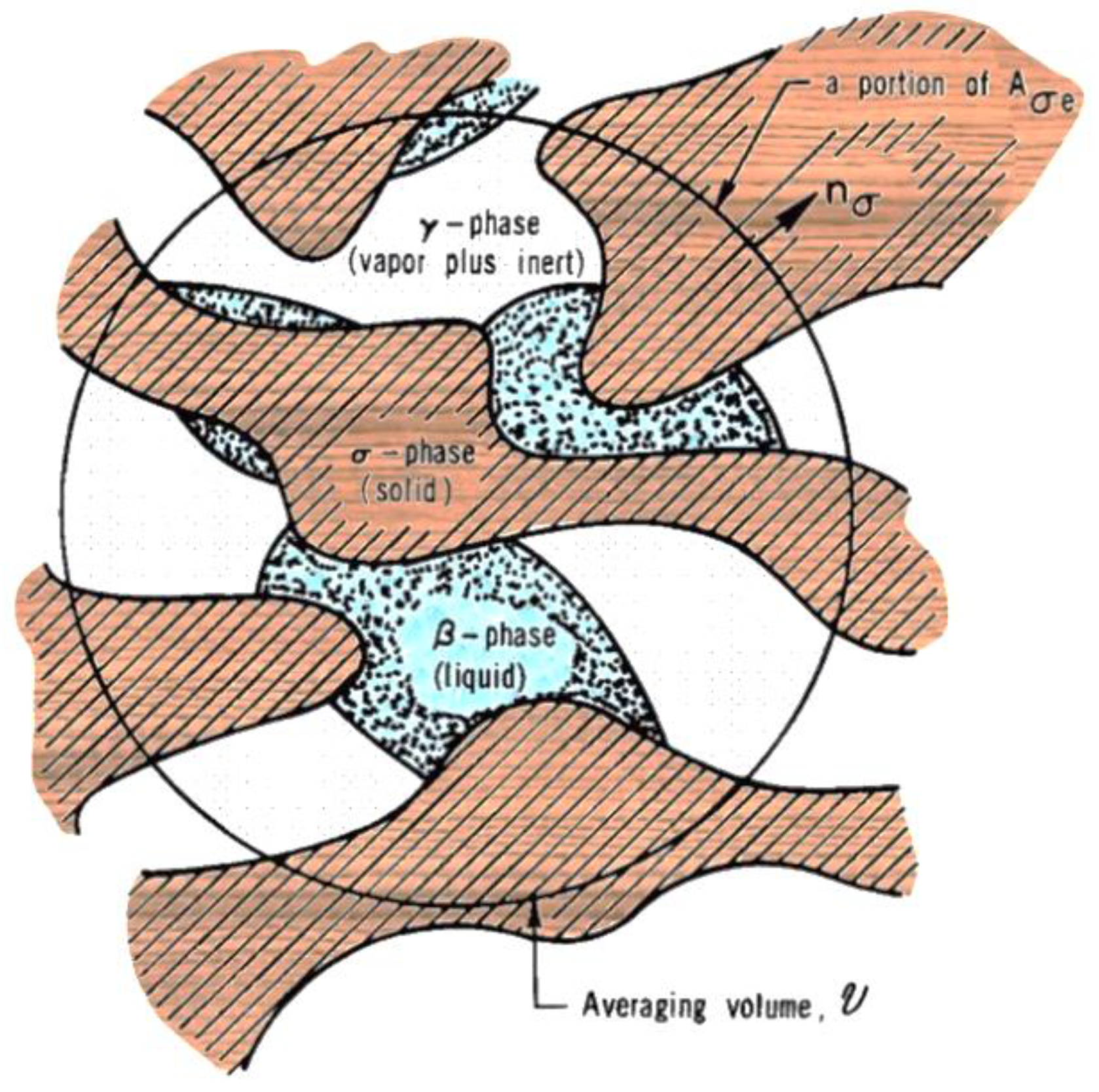
3.3. Model of Whitaker

In 1977, Stephen Whitaker [48] developed his theory of homogenization by analyzing the three phases of moisture and vapor movement in a rigid porous media, as shown in Figure 5. In Figure 5, σ represents the phase of the rigid solid matrix, β is the liquid phase, and γ shows the gas phase. Whitaker’s model concerned the topological structure of a three-phase system of equations, including liquid, vapor, and solid phases. There are three averaging methods that are useful in the analysis of heat and mass transport in porous media [80]. Whitaker provided the general form of the equations derived by the spatial volume averaging method. Whitaker’s equations were later simplified by several authors to facilitate experimental investigation of the theory. Perre [81] presented a simplified version of the equations under specific conditions, Whitaker’s theory can be described using coupled heat and moisture transfer models. The hygrothermal model of Whitaker can be expressed as follows:

$${\rho }_s\frac{\partial X}{\partial t} =\nabla ({\rho }_s f{D}_v \nabla {\omega }_v+D_b\nabla {\rho }_v-{\rho }_l \overline{V_l})$$

(20)

$$\frac{\partial ({\epsilon }_l{\rho }_l{h}_l+{\epsilon }_v{\rho }_v{h}_v+{\epsilon }_s{\rho }_s{h}_s+\overline{{\rho }_b}\overline{h_b})}{\partial t}=\nabla \left(\lambda \nabla T\right)+{h_v \rho }_v f{D}_v \nabla {\omega }_v+{\overline{h_b} D}_b\nabla {\rho }_v+h_l{\rho }_l \overline{V_l}$$

(21)

Like other models of energy and moisture conservation equations, the terms T and $X$ represent the temperature and mass moisture content. ${\rho }_s$, ${\rho }_v$, and ${\rho }_l$ are the densities of the porous material, vapor, and liquid, respectively. The symbols $f{, D}_v,$and $D_b$ are dimensionless diffusivity and the diffusivity of water vapor and bound water, respectively. The parameter ${\omega }_v$depicts the vapor mass fraction. The parameters of ${\epsilon }_l$, ${\epsilon }_v$, and ${\epsilon }_s$ are, respectively, the volume fraction of liquid, vapor, and solid, respectively. Similarly, $h_l$, $h_v{, h}_s$, and $h_b$ are the specific enthalpy of the liquid phase, vapor phase, solid phase of water, and specific enthalpy of bound water, respectively. Finally, $\lambda$ is the thermal conductivity of the porous body.

The moisture movement equation incorporates contributions from various mass transfer mechanisms, namely vapor diffusion, bound water diffusion, and mass convection. These mechanisms are considered in terms of enthalpies of each phase in the thermal energy equation.

3.4. Model of Künzel

In 1995, Künzel [46] proposed a new hygrothermal model during his PhD thesis. This model utilized relative humidity as the driving potential, a departure from the conventional approaches relying on volumetric water content and capillary pressure. Martin Krus’s thesis [82] investigated the various diffusion coefficients in hygrothermal transfer. A drawback of the models based on volumetric water content or capillary pressure is the discontinuity of the water content in multi-layered building components. Divergent jumps of the water content at the boundary layers between the two different materials require the computation of the moisture transport through complex transitional functions at the material boundaries. In a super-saturated region (highly saturated region), there is no straight relation between the water content and the driving potential for the liquid transport, as capillary suction stress may cause a wrong estimation. The hygrothermal model of Künzel based on relative humidity as the driving potential can be written as:

$${\xi }_{\phi }^{\theta } \frac{\partial \phi }{\partial t} =\nabla (D_{\phi } \nabla \phi +{\delta }_p \nabla (\phi p_{vs}))$$

(22)

$$C \frac{\partial T}{\partial t}=\nabla \left(\lambda \nabla T\right)+L \nabla ({\delta }_p·\nabla (\phi p_{vs}))$$

(23)

where ${ D}_{\phi }$ denotes the liquid conduction coefficient and can be calculated from the partial vapor pressure in the sorption region by the formula introduced in EN 15026 [83], $D_{\phi }=p_{vs}·{\delta }_p$. This only can be written in the sorption region under the isothermal condition when there is no liquid conduction through the pores during the capillary rising test. The relation between the capillary coefficient $D_W$, liquid water permeability $K,$and the liquid conduction coefficient ${ D}_{\phi }$in Künzel model is formulated below:

$$D_{\phi }=D_W {\xi }_{\phi }^{\theta } \frac{K{\rho }_l\mathfrak{R}T}{\phi }$$

(24)

where $D_W$can be determined by measuring transient moisture profiles in building materials, as explained in this reference [82]. The term liquid transport based on the temperature gradient was not considered by Künzel due to the small effect in comparison with the moisture gradient. This term was later applied by the Liu formulation based on the Künzel model using COMSOL and was well validated by comparing against the benchmark test of EN 15026 [83,84] and the benchmarks of the HAMSTAD project [85]. Hans Janssen [86] clarified that under isothermal conditions, Künzel’s and Liu’s equations yield equivalent results. Even in non-isothermal conditions, it can be also neglected due to small effect of temperature on moisture gradient. Dong et al. [87] compared the Künzel and Liu models with the HAMSTAD benchmark 5 and revealed that during high relative humidity, there is a slight deviation.

The advantages of the Künzel model are governed by the partial vapor pressure and relative humidity, both of which are material-independent variables and easy to measure during experiments. This model is the basis of the WUFI software [Wärme Und Feuchte Instationär, which, translated, means heat and moisture transiency] developed during Künzel’s PhD thesis. It has been utilized in numerous research works [6,88]. Künzel’s model as an engine of the WUFI software showed a good match with the experiments carried out in the Department of Hygrothermics at Fraunhofer IBP.

This model was later applied to the Energy Plus software version 8.2 as a HAM model for energy study of buildings. It was analyzed by the National Renewable Energy Laboratory (NREL) to better understand the different existing models in the EnergyPlus software [7]. Furthermore, there is a need for simpler moisture prediction models with fast response time and high accuracy. For this purpose, Woods et al. [89] analyzed the four models in Energy Plus, two different effective moisture penetration depth models (EMPD1 and EMPD2), effective capacitance (EC) model, and the Künzel model (HAM model). The results indicates that the Künzel model and two EMPD models were closer to the isothermal analytical solution.

Seong and Sumin [90] analyzed the impact of indoor temperature on moisture storage in the insulation layer in walls using the WUFI 6.7 software. For a wooden material, lower indoor temperature resulted in higher moisture storage. Zirkelbach et al. [91] applied the WUFI software for simulation of the different green roofs, considering the outdoor climate conditions, soil type, and drainage boards. The Künzel model was validated with the help of measured temperature and humidity field tests. Experimental measurements showed good agreement with the WUFI simulation results. Recent achievements and developments in relative humidity formulation include the three coupled models, or a complete form of heat, air, and moisture transfer (HAM models). These models consider forced convection for air transfer, and use relative humidity as moisture potential, such as HAM-Lea [92] and HAM-fit [93] models. In other research based on the humidity formulation of a hygrothermal model, Zhang et al. [52] took into account the temperature-dependent hysteresis effect. It was supposed that their models could more effectively illustrate the declining trend of moisture content.

3.5. Model of Rode

Rode Pedersen first presented the simplified system of equations of coupled heat and moisture transfer in his paper published in 1990 [47]; this model was implemented in the MATCH software. The coupled hygrothermal equations of Rode’s model are written as:

$${\rho }_0 \frac{\partial u}{\partial t} =\nabla (K_l \nabla {\psi }_p +{\delta }_p\nabla P_v)$$

(25)

$${\rho }_{0}c \frac{\partial T}{\partial t}=\nabla \left(\lambda \nabla T\right)+L \nabla (K_l\nabla {\psi }_p)$$

(26)

where $K_l$is the hydraulic conductivity as a function of water content. Moreover, the model also considered the hysteresis of the moisture retention curve by taking into account both adsorption and desorption curves. In addition, it defines the moisture capacity as a function of the water content and direction of the retention process (adsorption/desorption). A procedure was introduced for hysteresis in the sorption curve, though it is equally valid for the suction curve as well.

3.6. Model of Grunewald

The Grunewald model was initially shown in [49], while its numerical implementation, considering new features also with dry air transport and a focus on pollutant and VOC (volatile organic compound) transport, was later included in the software. This model is implemented in the software Delphin 5 and in its later versions as written as:

$$\frac{\partial u}{\partial t} =\nabla (K_l\nabla {\psi }_p +\frac{{\delta }_p{P}_{ vs} \mathrm{e}\mathrm{x}\mathrm{p}(\frac{{\psi }_p}{{\rho }_l\mathfrak{R}T}) }{\mathfrak{R}T}.\nabla {\psi }_p)$$

(27)

$$C \frac{\partial T}{\partial t}=\nabla \left(\lambda \nabla T\right)+L \nabla (\frac{{\delta }_p{P}_{ vs} \mathrm{e}\mathrm{x}\mathrm{p}(\frac{{\psi }_p}{{\rho }_l\mathfrak{R}T}) }{\mathfrak{R}T}\nabla {\psi }_p)$$

(28)

It can simulate transient mass and energy transport processes for arbitrary standard and natural climatic boundary conditions by considering the wind-driven rain, wind speed, wind direction, and short- and long-wave radiation. Hejazi et al. [94] compared the two well-known softwares WUFI Pro 4.2 and DELPHIN (Version 5) in the case of validation. And the results obtained from two softwares were very close. One of the advantages of capillary pressure form of hygrothermal equations is in a saturated region where we have a higher relative humidity. In this region, capillary pressure can define the state of the water content in the material. An example of recent models is Fang et al. [51], who used capillary pressure as the single driving potential for both vapor and liquid transport to predict wind driving rain penetration.

4. Discussion on Building Hygrothermal Models

Coupled heat and moisture transfer is governed based on the principles of energy and mass conservation, along with diffusion equations and a few state equations. In

Table 2. Summary of hygrothermal models.

Name of Model	Year	Moisture Transfer Driving Potential	Moisture Phase
Richard’s equation	1931	Capillary pressure	Only liquid phase
Philip and De Vries model	1957	Water content	Liquid + vapor phases
Luikov model	1965–1974	Water content	Liquid + vapor phases
Sophocleous and Milly’s model	1977, 1982	Capillary pressure	Liquid + vapor phases
Whitaker’s model	1977	Water content	Liquid + vapor + solid phases
Künzel model	1995	Relative humidity	Liquid + vapor phases
Model of Rode	1992	Vapor pressure–capillary pressure	Liquid + vapor phases
Model of Grunewald	1997	Capillary pressure	Liquid + vapor phases

, a summary of the hygrothermal equations outlined in this review is presented. The equations inspired by the theory of Philip and De Vries are based on the assumption that the moisture transfer could be classified into a liquid phase and vapor phase flow. Since then, it has been challenging that there is no way to directly measure these two phases in a pore system. To deal with this, Luikov, for instance, assumed that the two phases are assumed to be proportional, with the proportionality factor as a (fitted) constant. Luikov developed the system of coupled heat and moisture equations based on the irreversible thermodynamics law (Gibb’s theory). Richard’s equation, together with the Fourier equation, created one of the first hygrothermal models in 1931; however, the exclusion of condensation, evaporation, and the vapor phase of water in the analysis may have led to potentially misleading results.

On the left-hand side of the equations, the storage dependency is defined and provides a relationship between the volumetric water content and relative humidity or the relationship with the capillary suction pressure, which comes from the sorption isotherms of material or retention curve. For instance, in both Künzel’s model and Sophocleous and Milly’s model, which consider the moisture transport with the driving forces of humidity and capillary pressure, this relationship was provided by derivation of sorption isotherm ($\frac{\partial \theta }{\partial \phi }\ast \frac{\partial \phi }{\partial \mathrm{t}}$) and water retention curve ($\frac{\partial \theta }{\partial {\psi }_p}\ast \frac{\partial {\psi }_p}{\partial t}$). The derivations of $\frac{\partial \theta }{\partial \phi }$ and $\frac{\partial \theta }{\partial {\psi }_p}$ are equal to the slope of the sorption curve and water retention curve, which is known as the specific volumetric moisture capacity (${\xi }_{{\psi }_p}^w$, ${\xi }_{\phi }^w$). For converting the sorption isotherm curve as a function of capillary suction, Kelvin’s equation is also applicable to link the capillary suction to relative humidity: ${\psi }_p={\rho }_l\mathfrak{R}TLn\left(\phi \right)$. Luikov’s model for colloidal porous materials, published in 1966, introduced the two terms of moisture and heat propagation factors (${\tau }_{rm}$, ${\mathsf{\tau }}_{\mathrm{r}}$), which can be neglected in building materials. It only became significant under certain conditions; however, its exceptional value renders laboratory measurements impractical.

Physical parameters comprising $D_T$ and $D_{\theta }$ are defined in all models in some way, representing the general diffusion coefficients for heat and moisture gradients and separated as $D_T=D_{T,v}+D_{T,l}$ and $D_{\theta }=D_{\theta ,v}+D_{\theta ,l}$. The coefficients of $D_{T,V} \mathrm{a}\mathrm{n}\mathrm{d} D_{T,l}$are the diffusivity of liquid and vapor under the temperature gradient. $D_{T,l}$ was neglected in the Luikov, Philip and De Vries, Künzel, and Rhode models due to the low value of the liquid transfer in the temperature gradient. One of the differences between Rhode’s model in a comparison of others is the term coupling in the heat equation ($L \nabla (K_l\nabla {\psi }_p)$), which is defined as the liquid transfer instead of considering the vapor transfer. Luikov’s model in 1965 for building materials came with the coefficient of ($\lambda +L{D}_{T,v}$) for the thermal transfer, and later, for capillary porous materials, Luikov transferred the thermal equation by adding $\frac{\partial \theta }{\partial t}$, which is a complete coupled equation. This transformation on hygrothermal models has not been compared yet to see how it affects the temperature and moisture content distribution in both multilayer materials and single-layer ones. In Luikov’s system of equations, and especially in the general form, there was a lack of physical definition on diffusion coefficients under the temperature or moisture gradient. Künzel explained the disadvantages of utilizing the water content as the driving potential in multilayer material, which is the discontinuity of water content at the interface of multi-layered building materials [47]. In Figure 6, a concept of Künzel’s view on multi-layered building materials is presented; there is a rise in water content from material 1 to material 2, in a comparison of humidity with a smooth variance in the boundary layer.

One of the disadvantages of relative humidity models comes in the supersaturated region. As stated in [95], relative humidity is deemed unsuitable as a potential variable to be chosen due to the high slope of the moisture retention curve after 99% (or in the supersaturated region). Even slight fluctuations in relative humidity can lead to considerable variations in moisture content, necessitating the use of ten or more significant digits for accurate measurements. Relative humidity formulation could be suitable for the sorption region, and during the rain or any durability analysis of building wall construction, it might cause a wrong estimation.

The state of the equilibrium moisture content of a capillary body depends on the temperature and humidity of the surrounding air and on the method of reaching equilibrium. The mechanism of transfer varies depending on how the equilibrium condition is reached. Thus, the maximum hygroscopic moisture content of any porous media, corresponding to the porous body with humidity of 100%, is significantly less than the maximum moisture content that the body can acquire in absorbing water or by wettability of the porous media. A similar relation holds for coarse-pored bodies such as building materials. This equilibrium moisture content would decrease by increasing the temperature, and during the hygroscopic equilibrium condition, various mechanisms affect the moisture transfer, monolayer adsorption in the range of 0–10% humidity, polymolecular adsorption in the range of 10–90% humidity, and capillary transport in the range of 90–100% humidity (see Figure 7). This hysteresis could be relatively varied from one geometry of pore to another. An inherent challenge in the classification of regions within hygroscopic materials, as illustrated in Figure 7, stems from the absence of a definitive rule for characterizing various regions from sorption to super-saturated.

Several related areas in the hygrothermal modeling need further scrutiny:

• Considering the three-dimensional hygrothermal analysis with an additional term of infiltration or air velocity in porous media.
• Taking into account the computational fluid dynamics (CFD) approach rather than the conventional 1D methods because the power of the computers has been improved. CFD offers detailed information on airflow, temperature, and humidity throughout the building environments and constructions.
• It is also not clear yet what the hysteresis effect is of sorption/desorption in moisture risk analysis of building materials.
• International efforts are needed to bring attention to assessing the hygrothermal models on various climate regions, especially in cold freezing regions.
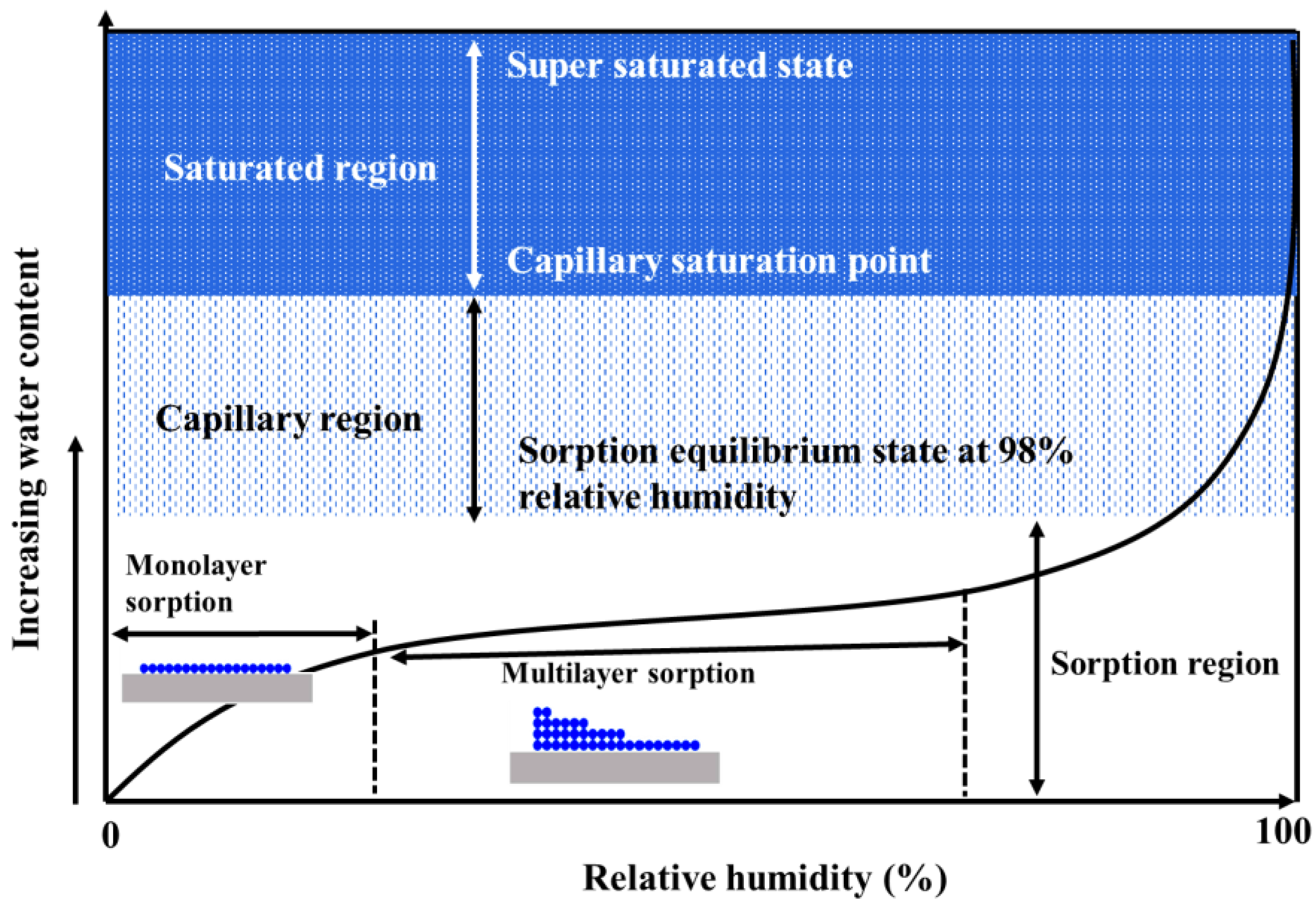
• The development of hygrothermal models encompasses all moisture states in porous materials, including the sorption, capillary, and saturated regions.

5. Advancements from Glaser Method to EN ISO 15026

The goal of hygrothermal simulation in the building sector is to evaluate the variation in temperature and moisture within porous building materials, with precise consideration of the ambient humidity, initial conditions, and energy exchange between the inside of the envelope and the surrounding environment. Future objectives include quantifying the energy consumption of buildings, thermal comfort, durability, and indoor air quality issues [96]. A poorly designed building can result in surface condensation, posing a significant risk of mold growth. Also, the risk of condensation is considerably affected by age and height of materials used in the building, especially old ones. In order to ensure the health and safety of building occupants, it is necessary to control moisture migration and accumulation inside building envelopes [97]. As part of this section, one of the hygrothermal applications in building envelopes is discussed which has finally become a standard in various countries. Furthermore, we present a brief discussion on how the classic graphical method, known as the dew point method, transformed into the transient hygrothermal method. All the efforts came from this truth to accelerate the building simulation and reach a trusted hygrothermal model.

By the end of 1940, Rowley, Algren, and Lund [96] introduced the graphical method, known as the steady-state method, which was subsequently applied in practice by Johansson and Persson, Egner [97], Cammerer and Diirhammer [98]. This method was used for the occurrence of condensation in building construction. They defined vapor pressure curves based on the vapor permeance of materials. After World War 2, the graphical method found application in Europe, operating under the assumption that condensate was deposited through the building material with the water vapor saturation line and every assembly with some insulation layer needed a vapor barrier. Due to the unsatisfactory results of their approach, Helmut Glaser published four papers between 1958 and 1959 [99,100,101,102] to develop this simple method to control interstitial condensation in moisture-safe freezer walls based on steady-state vapor diffusion. The Glaser method, which is originally a graphical method, calculates moisture transfer as steady-state diffusion after a steady-state thermal calculation has been carried out.

Figure 8 schematically demonstrates a cellular concrete in a Glaser method analysis, covered with insulation or roofing material on the exterior side during winter. We suppose the cellular concrete to be exposed to high relative humidity and low temperature on the exterior side ($T_{exterior}$) exchange with high temperature and low relative humidity inside ($T_{interior}$). The vapor pressure profile can be calculated from the differences between the interior and exterior vapor pressure ($P_{V.exterior}-P_{V.interior}$) over the vapor diffusion resistance. Due to the high resistance factor on the upper side, the vapor pressure differences almost established themselves over the roof. Additionally, saturation pressure is only dependent on temperature, as shown by the dotted line in Figure 8. As a result of this graphical method, by comparing the vapor saturation and distribution, in the upper part of the roof, the vapor pressure is higher than the saturation vapor pressure, so the blue highlighted color in Figure 8 shows where condensation can be expected [103,104].

This simple, one-dimensional, steady-state calculation approach has been implemented in standards and codes in Europe, the USA, and Canada. The Glaser method was known as the “dew point method” in Canada and the USA. The standard of EN ISO 13788, first introduced in Belgium and the Netherlands, is now part of the European standards for internal surface temperature to avoid interstitial condensation and critical surface humidity [105]. As is known, this method has a lot of limitations and does not include a number of important physical phenomena [104]:

• The variation of material properties with moisture content;
• Capillary suction and liquid moisture transfer, which whiten materials;
• Air movement from within the building into the component through gaps or air spaces;
• Hygroscopic moisture capacity of materials.

None of the conditions were met, yet the simplicity of the Glaser approach was charming. This attracted the researcher’s interest in upgrading the Glaser method in the years following the 1950s, with significant contributions from Vos in 1969 and 1971 [106,107] and Hens in 1975 and 1978 [108,109], Van der Kooi in 1971 [110], and Kieβl in 1983 [111].

Since the 1990s, advances in power and speed have opened the way for the development of comprehensive models capable of transient or non-steady-state-coupled heat and moisture transfer (discussed in Section 2) in one-dimensional to three-dimensional multilayer composite building materials. Some of these models are commercialized, such as WUFI software, as discussed in Section 3 [112]. Figure 9 summarizes international efforts from 1990 to 2007 to explore hygrothermal phenomena in building physics. Despite the progress, due to the complexity of the phenomena and the models, the hygrothermal phenomenon is not mathematically well modeled and is still under development. The first effort is Annex 24: Heat, Air and Moisture Transfer in Envelopes (HAMTIE), which was initiated by the International Energy Agency (IEA) organized in 1990. The main objective of Annex 24 was to analyze the effect of HAM response on thermal performance and durability in buildings and to study the physics of heat, air, and moisture transport. Later in 2001, the European Commission initiated the project “HAMSTAD “(Heat Air and Moisture Standard Development), which focused on the development of draft standardization procedures for determination methods of moisture transfer properties and draft methodology for certification of upgrading moisture modeling codes. As a result of the Annex 24 meeting in Paris, in April 1991, five benchmark reports were published [113,114]. The HAMSTAD project, in contrast to Annex 24, includes two phases: an open methodology for free code development and the quality assessment of codes. This project aims to implement a better HAM modeling methodology than the traditional Glaser approach [85]. The recent international effort is IEA ECBCS Annex 41 from 2003 to 2007, by taking into account the various models in “whole buildings” and considering the advanced development in modeling the heat, air, and moisture transfer [115,116,117]. Six different exercises were carried out in this international project to make intermodel comparisons and validate the results with experimental data [114].

The results proposed in the HAMSTAD project led to the upgrading or revision of (pre-)EN standards for measuring the moisture transfer coefficients, water vapor permeability [118], sorption–desorption curves, and water retention curves [119]. In contrast to steady-state assessment or the graphical method introduced by Glaser, now as part of the European Standard [104], transient hygrothermal simulation brought more details and precise analysis on the risk of moisture issues within the building constructions and materials. Transient assessment of the hygrothermal performance of building components covered in European Standard EN 15026 accounts for heat and moisture storage, sensible latent heat, vapor and liquid transfer under the realistic boundary, and initial condition. Annex A of EN 15026 [83] defines a normative benchmark test to ensure that the software and code used fulfills some basic requirements and provides accurate results. This benchmark is based on the analytical solution for hygrothermal transfer in a semi-infinite region named here as “No.6 Analytical case 2” in Section 5.6 [120].

In the following sections, we revisit and summarize the six important benchmarks developed during the HAMSTAD project and European Standard EN 15026. Each benchmark covers at least two transfer mechanisms. These benchmarks follow the hygrothermal model considering the liquid and vapor transfer for moisture formulation and serve as the basis for numerical solutions. They also cover air transfer and heat and mass balance, as well as exterior and interior boundary and climate conditions. It must be kept in mind that several equations can characterize the moisture state, such as water vapor pressure, capillary pressure, relative humidity, and volumetric water content, and relate them to each other. All these driving potentials should be able to determine the moisture content as a result. It is a complicated task due to the nonlinearity of the hygrothermal equations and it requires a solid understanding of both mathematics and the physical properties of the parameters involved. However, various numerical results in the benchmark cases showed that reasonable consensus solutions can be found. Reference [85] provide more details on the initial boundary conditions and physical properties of materials in HAMSTAD benchmarks.

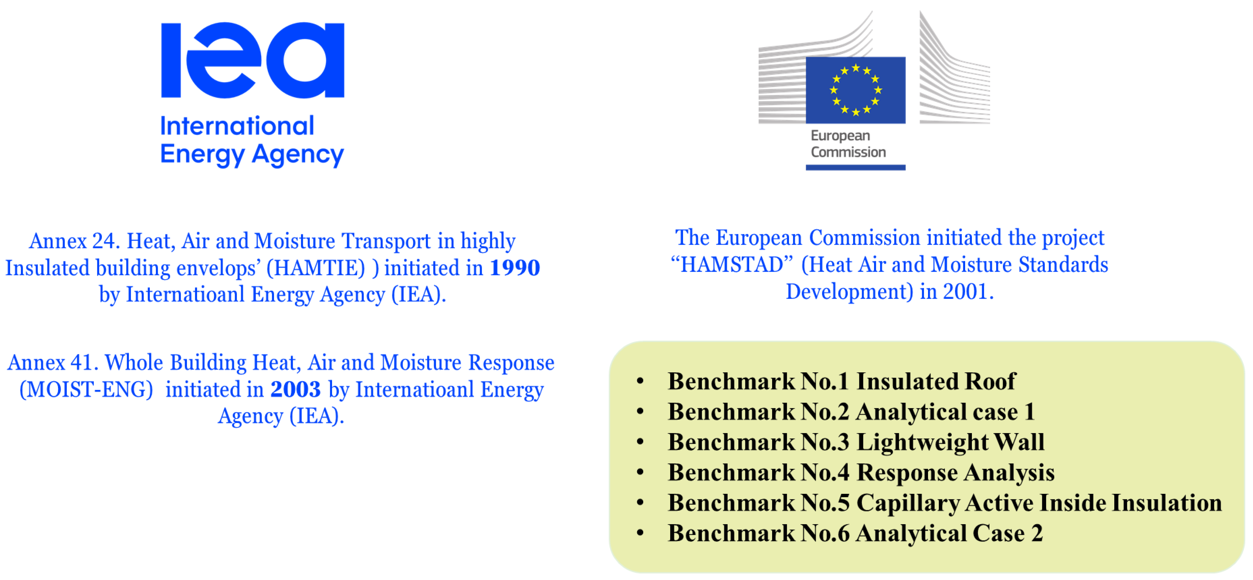
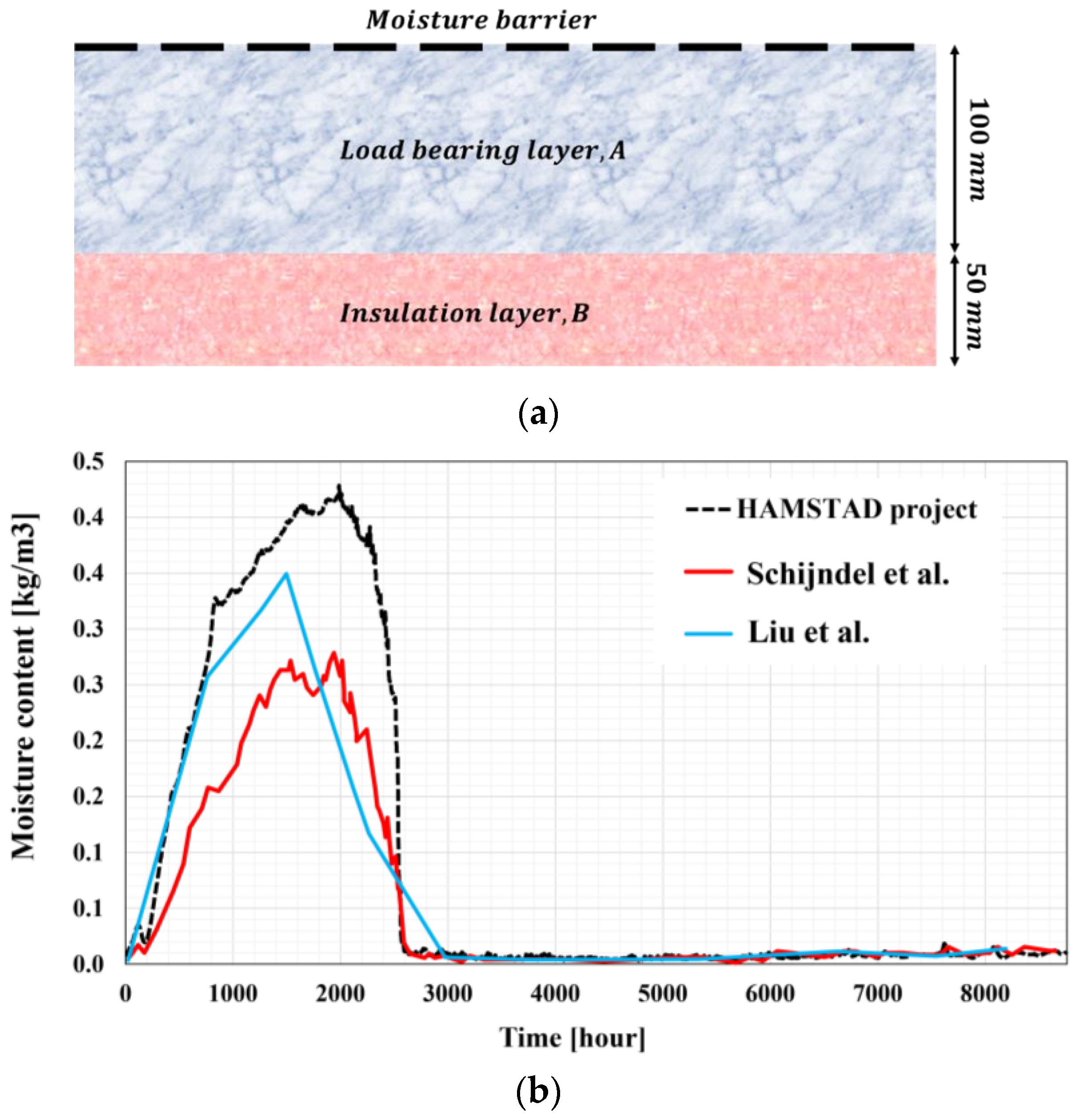
5.1. Benchmark No. 1 Insulated Roof

This benchmark addresses interstitial condensation that arises at the interface between two materials. The construction assembly consists of a vapor-tight seal, a 100 mm load-bearing material, and a 50 mm thermal insulation layer. The assembly of the roof structure is shown in Figure 10a. The properties of the two materials differ; the load-bearing layer is capillary-active, while the hygroscopic insulation is capillary-non-active. Thermal conductivities between two materials differ by a factor of 50 (at dry conditions). The simulation covers five years with a normal external climate fluctuation. Even though there is good agreement of the results of the moisture content in the load bearing layer, the results in the insulation layer disperse from year to year (Figure 10b).

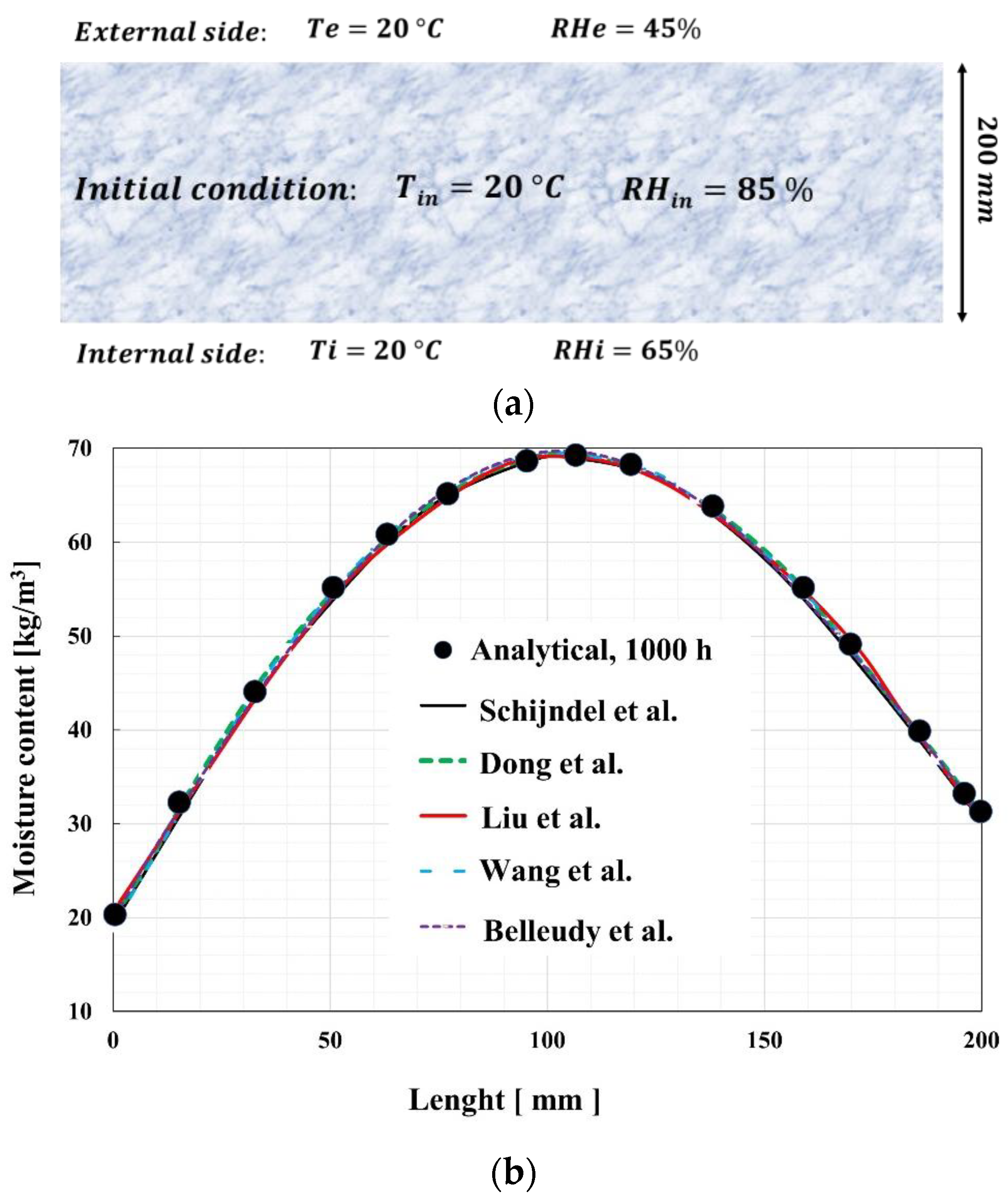
5.2. Benchmark No. 2 Analytical Case 1

This benchmark concerns the moisture redistribution in a homogeneous material with the thickness of 200 mm under isothermal conditions (shown in Figure 11a). Initially, the moisture equilibrium of the layer is maintained by the relative humidity of the ambient air, which is kept constant. The movement of moisture results from a sudden change in relative humidity in the environment, causing a swift but different change in humidity. This case can be solved analytically, with the initial conditions of 20 °C and relative humidity of 85%. Temperature is kept constant at the boundary conditions, while humidity varies from 45% to 65%. As shown in Figure 10b, the simulation covers 1000 h for the calculation of the moisture content through the wall. However, [88] illustrates the results for 100 and 300 h.

5.3. Benchmark No. 3 Lightweight Wall

In the third benchmark, air is transferred through a single layer of 200 mm thickness. Airflow is the main cause of moisture transfer in this case, but moisture and temperature gradients across the layer also play a role in the heat and moisture transfer. The boundary conditions are constant, except for the pressure difference between indoor and outdoor, which causes the infiltration or convection of air. Over the initial 20 days, air exfiltration occurs, which subsequently transitions into air infiltration. Further information regarding boundary conditions is presented in Figure 12a and in [85]. As a result of the third benchmark, moisture distribution during the 100 days is shown in Figure 11b.

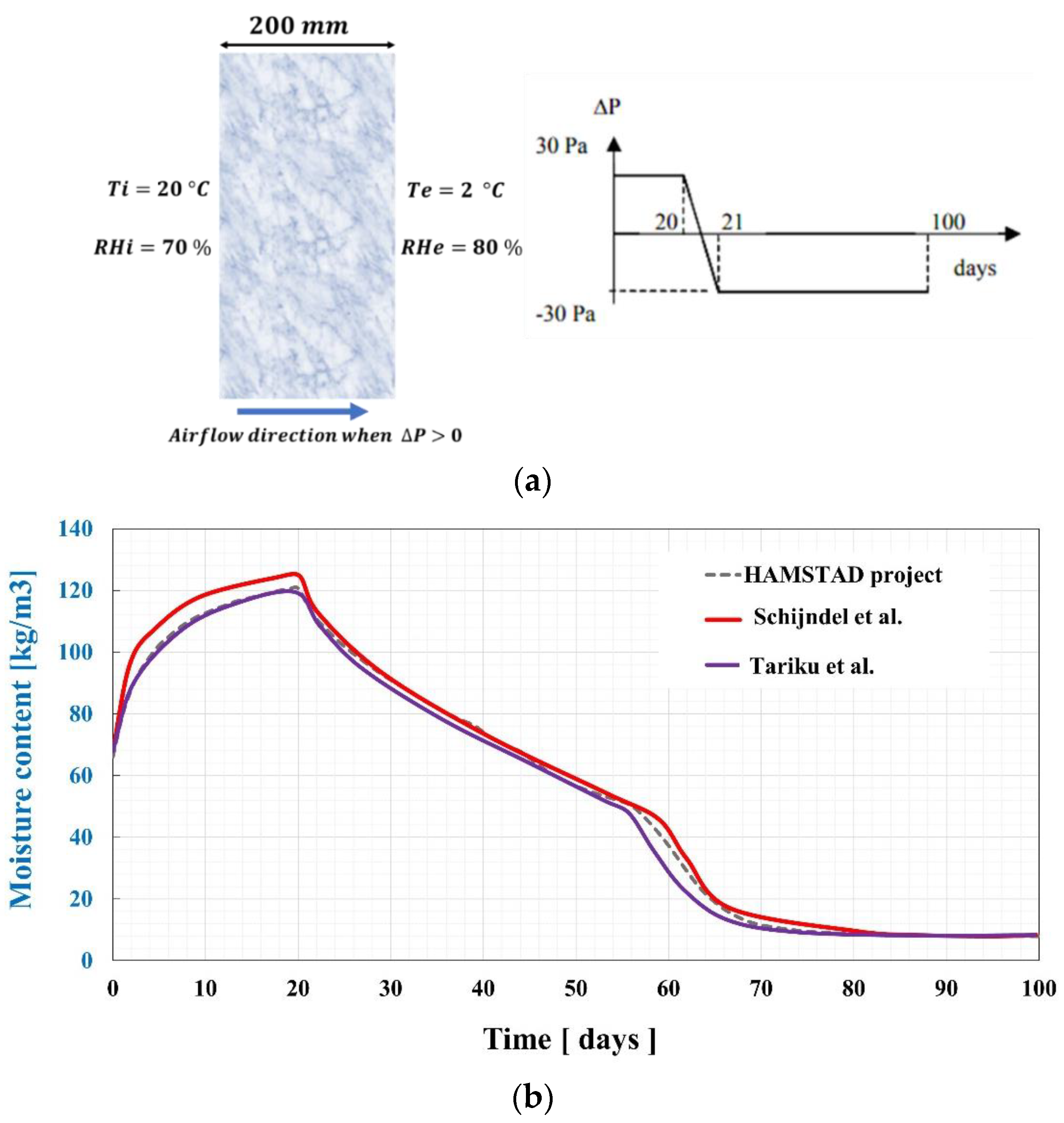
5.4. Benchmark No. 4 Response Analysis

The fourth benchmark consists of a 100 mm wall with a 20 mm plaster on the inside, which is subjected to rain and solar irradiation (see Figure 13a for schematic view of geometry). There is no convective heat and moisture throughout the layer. During the 24 h simulation period, the climatic conditions are quite harsh, causing a different heat and moisture transfer, such as moisture condensation and redistribution of moisture between the interface of the two capillary materials. References [85,121] provide a detailed description of the material data and climatic conditions for this benchmark. Figure 13b is presented here for just moisture distribution during the 100 days; various researchers simulated this benchmark.

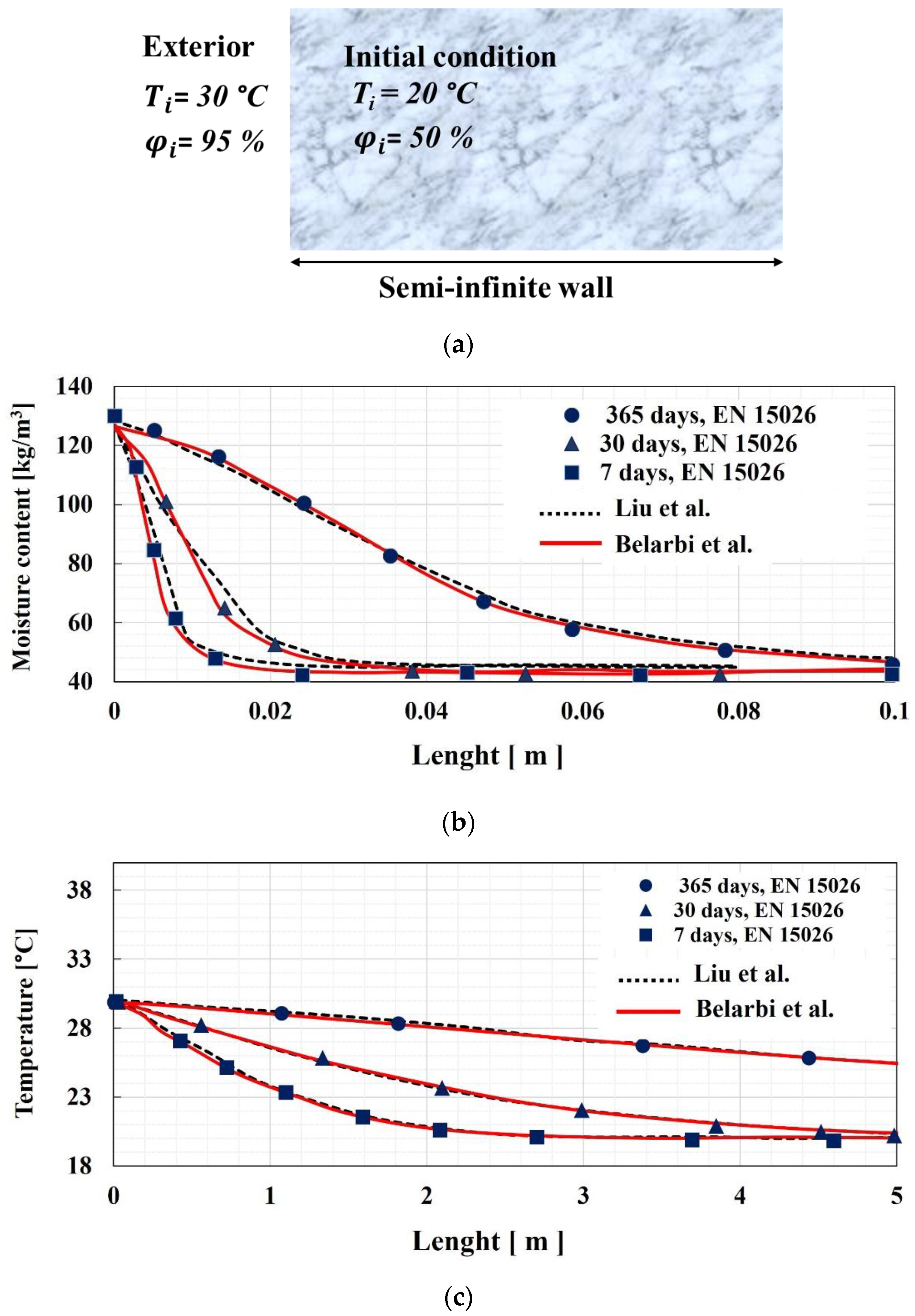
5.5. Benchmark No. 5 Capillary Active Inside Insulation

The fifth benchmark addresses the moisture redistribution inside a wall with highly hygroscopic interior materials. The wall assembly includes three different materials, as shown in Figure 14a. A constant initial temperature and water content are considered throughout the wall with a sudden change in temperature and water vapor pressure at the starting point of the simulation. Two different numerical solutions agree well for all layers during the 60 days chosen for the simulation. As a result of this benchmark, Figure 14b illustrates the moisture profile through the wall construction. As moisture content varies in the wall construction, there is a sharp enhancement in the insulation material due to the various physical properties of the insulation material and mortar, including the sorption isotherms and water vapor permeability.

5.6. Benchmark No. 6 Analytical Case 2

The sixth benchmark introduced in ISO EN 15026 deals with coupled heat and moisture transfer in a semi-infinite material (thick building material). Climate, whether or not in the boundary condition, is constant and the materials are airtight. Figure 15a shows the boundary conditions of this benchmark. At a certain time (7, 30, 365 days), temperature and moisture profiles were calculated with an analytical solution (see Figure 15b and Figure 14c) [83].

6. Conclusions

Nowadays, hygrothermal models have been and continue to be a research subject in the building sector due to their inseparable role in building energy analysis. Developments in heat and moisture modeling have progressed since 1907 when Buckingham introduced the “capillary potential” as a driving force for moisture movement in un-saturated soil. Parallel to research in unsaturated soil, hygrothermal models were also under development. Later, in the 1950s, Philip and De Vries brought a novel form of hygrothermal equations by considering the vapor phase and sensible latent heat in their theory. Due to the limitations of this study, only the most utilized and well-known hygrothermal models developed after the theory of Philip and De Vries are discussed, including Milly’s model, Luikov’s models, Whitaker’s model, Sophocleous and Milly’s model, Rode’s model, Künzel’s model, and Grunewal’s model. Most of these models have been experimentally and numerically analyzed as computer technology advanced, proving their accuracy by providing reliable results. The strength of this literature review lies in its comparison of these hygrothermal models, detailing their utility and downsides. Künzel’s model is not the latest version of the hygrothermal model with humidity formulation, but it can be a starting point for researchers to develop and fill this research gap by providing solutions that are not only advanced and complicated but also easy to apply. Whitaker’s model, for the first time, incorporated the effect of rigid porous media in the hygrothermal equations. It should be mentioned that it is complex and still lacks an experimental procedure for verifying the accuracy of this formulation. Due to variations in computing techniques, as evidenced by comparing the results of HAMSTAD benchmarks produced with different numerical solutions, the results might vary from one to another. The methods and algorithms used for numerical solutions, mesh elements, boundary conditions, and the variety of coefficients are parameters influencing numerical modeling. Hygrothermal models have been widely used in the building sector to analyze condensation occurrences in building components. Efforts by authors in the mid-1940s led to the introduction of a graphical method later developed by H. Glaser, which calculates moisture transfer as steady-state diffusion, also known as the “dew point method” in the USA and Canada. Despite its simplicity, this graphical method produced unsatisfactory results. International efforts, such as Annex 24 starting in 1991 and the HAMSTAD project in Europe in 2001, led to the development of better and more accurate methods for moisture risk analysis in building applications. Six different benchmarks were introduced to ensure that the software and codes used meet basic requirements and provide accurate results in transient hygrothermal assessments. These proposed codes and benchmarks were later included in the upgrade or revision of (pre-)EN standards. In conclusion, the present study, with the provided information, aims to guide researchers and engineers engaged in building analysis as well as those aiming to develop novel hygrothermal models.

References

1. Aceti, P.; Carminati, L.; Bettini, P.; Sala, G. Hygrothermal Ageing of Composite Structures. Part 1: Technical Review. Compos. Struct. 2023, 319, 117076. [Google Scholar] [CrossRef]
2. Su, Y.; Tian, M.; Li, J.; Zhang, X.; Zhao, P. Numerical Study of Heat and Moisture Transfer in Thermal Protective Clothing against a Coupled Thermal Hazardous Environment. Int. J. Heat Mass Transf. 2022, 194, 122989. [Google Scholar] [CrossRef]
3. Tadeu, A.; Simões, N.; Branco, F. Steady-State Moisture Diffusion in Curved Walls, in the Absence of Condensate Flow, via the BEM: A Practical Civil Engineering Approach (Glaser Method). Build. Environ. 2003, 38, 677–688. [Google Scholar] [CrossRef]
4. Blocken, B.; Roels, S.; Carmeliet, J. A Combined CFD–HAM Approach for Wind-Driven Rain on Building Facades. J. Wind Eng. Ind. Aerodyn. 2007, 95, 585–607. [Google Scholar] [CrossRef]
5. Janssen, H.; Blocken, B.; Roels, S.; Carmeliet, J. Wind-Driven Rain as a Boundary Condition for HAM Simulations: Analysis of Simplified Modelling Approaches. Build. Environ. 2007, 42, 1555–1567. [Google Scholar] [CrossRef]
6. WUFI. Available online: https://wufi.de/en/ (accessed on 11 June 2024).
7. EnergyPlus. Available online: https://energyplus.net/ (accessed on 11 June 2024).
8. Chkeir, A.; Bouzidi, Y.; Akili, Z.E.; Charafeddine, M.; Kashmar, Z. Assessment of Thermal Comfort in the Traditional and Contemporary Houses in Byblos: A Comparative Study. Energy Built Environ. 2024, 5, 933–945. [Google Scholar] [CrossRef]
9. Jiang, Q.; Li, Q.; Zhang, C.; Wang, J.; Dou, Z.; Chen, A.; Yang, Y.; Ren, H.; Zhang, L. Excavation of Building Energy Conservation in University Based on Energy Use Behavior Analysis. Energy Build. 2023, 280, 112726. [Google Scholar] [CrossRef]
10. Du, C.; Wang, Y.; Li, B.; Xu, M.; Sadrizadeh, S. Grey Image Recognition-Based Mold Growth Assessment on the Surface of Typical Building Materials Responding to Dynamic Thermal Conditions. Build. Environ. 2023, 243, 110682. [Google Scholar] [CrossRef]
11. Boonen, E.; Beeldens, A.; Dirkx, I.; Bams, V. Durability of Cementitious Photocatalytic Building Materials. Catal. Today 2017, 287, 196–202. [Google Scholar] [CrossRef]
12. Adilkhanova, I.; Santamouris, M.; Yun, G.Y. Coupling Urban Climate Modeling and City-Scale Building Energy Simulations with the Statistical Analysis: Climate and Energy Implications of High Albedo Materials in Seoul. Energy Build. 2023, 290, 113092. [Google Scholar] [CrossRef]
13. Aparicio-Fernández, C.; Torner, M.E.; Cañada-Soriano, M.; Vivancos, J.-L. Analysis of the Energy Performance Strategies in a Historical Building Used as a Music School. Dev. Built Environ. 2023, 15, 100195. [Google Scholar] [CrossRef]
14. Kalair, A.R.; Seyedmahmoudian, M.; Stojcevski, A.; Mekhilef, S.; Abas, N.; Koh, K. Thermal Comfort Analysis of a Trombe Wall Integrated Multi-Energy Nanogrid Building. J. Build. Eng. 2023, 78, 107623. [Google Scholar] [CrossRef]
15. Aggarwal, C.; Ge, H.; Defo, M. Assessing Mould Growth Risk of Wood-Frame Walls Using Partial Least Squares (PLS) Regression Considering Climate Model Uncertainties. Build. Environ. 2023, 238, 110374. [Google Scholar] [CrossRef]
16. Friis, N.K.; Møller, E.B.; Lading, T. Hygrothermal Conditions in the Facades of Residential Buildings in Nuuk and Sisimiut. Build. Environ. 2023, 243, 110686. [Google Scholar] [CrossRef]
17. Boardman, C.R.; Glass, S.V.; Lepage, R. Dose-Response Simple Isopleth for Mold (DR SIM): A Dynamic Mold Growth Model for Moisture Risk Assessment. J. Build. Eng. 2023, 68, 106092. [Google Scholar] [CrossRef]
18. Urso, A.; Evola, G.; Costanzo, V.; Nocera, F. A Critical Analysis on the Use of Different Weather Datasets to Assess Moisture-Related Risks in Building Components for a Mediterranean Location. J. Build. Eng. 2023, 76, 107177. [Google Scholar] [CrossRef]
19. Panico, S.; Larcher, M.; Herrera Avellanosa, D.; Baglivo, C.; Troi, A.; Maria Congedo, P. Hygrothermal Simulation Challenges: Assessing Boundary Condition Choices in Retrofitting Historic European Buildings. Energy Build. 2023, 297, 113464. [Google Scholar] [CrossRef]
20. Urso, A.; Costanzo, V.; Nocera, F.; Evola, G. Moisture-Related Risks in Wood-Based Retrofit Solutions in a Mediterranean Climate: Design Recommendations. Sustainability 2022, 14, 14706. [Google Scholar] [CrossRef]
21. Vandemeulebroucke, I.; Caluwaerts, S.; Van Den Bossche, N. Decision Framework to Select Moisture Reference Years for Hygrothermal Simulations. Build. Environ. 2022, 218, 109080. [Google Scholar] [CrossRef]
22. Libralato, M.; De Angelis, A.; D’Agaro, P.; Cortella, G.; Saro, O. Multiyear Hygrothermal Performance Simulation of Historic Building Envelopes. IOP Conf. Ser. Earth Environ. Sci. 2021, 863, 012045. [Google Scholar] [CrossRef]
23. Libralato, M.; De Angelis, A.; Tornello, G.; Saro, O.; D’Agaro, P.; Cortella, G. Evaluation of Multiyear Weather Data Effects on Hygrothermal Building Energy Simulations Using WUFI Plus. Energies 2021, 14, 7157. [Google Scholar] [CrossRef]
24. Zeng, L.; Chen, Y.; Cao, C.; Lv, L.; Gao, J.; Li, J.; Zhang, C. Influence of Materials’ Hygric Properties on the Hygrothermal Performance of Internal Thermal Insulation Composite Systems. Energy Built Environ. 2023, 4, 315–327. [Google Scholar] [CrossRef]
25. Philip, J.R.; De Vries, D.A. Moisture Movement in Porous Materials under Temperature Gradients. Trans. Am. Geophys. Union 1957, 38, 222. [Google Scholar] [CrossRef]
26. Ng, C.W.W.; Menzies, B. Advanced Unsaturated Soil Mechanics and Engineering; CRC Press: Boca Raton, FL, USA, 2014; ISBN 978-0-203-93972-7. [Google Scholar]
27. Ren, F.; Zhou, C.; Zeng, Q.; Wang, Z.; Wang, W. Numerical Investigations into the Physical Significance of Sorptivity for Cement-Based Materials Considering Water Sensitivity. J. Build. Eng. 2023, 66, 105952. [Google Scholar] [CrossRef]
28. Hamrouni, I.; Ouahbi, T.; El Hajjar, A.; Taibi, S.; Jamei, M.; Zenzri, H. Water Vapor Permeability of Flax Fibers Reinforced Raw Earth: Experimental and Micro-Macro Modeling. Eur. J. Environ. Civ. Eng. 2023, 27, 3020–3039. [Google Scholar] [CrossRef]
29. Carman, P.C. Fluid Flow through Granular Beds. Chem. Eng. Res. Des. 1997, 75, S32–S48. [Google Scholar] [CrossRef]
30. Ruan, K.; Fu, X.-L. A Modified Kozeny–Carman Equation for Predicting Saturated Hydraulic Conductivity of Compacted Bentonite in Confined Condition. J. Rock Mech. Geotech. Eng. 2022, 14, 984–993. [Google Scholar] [CrossRef]
31. Khan, W.A.; Yusuf, T.A.; Mabood, F.; Siddiq, M.K.; Shehzad, S.A. Chemically Reactive Water-Based Carbon Nanotubes Flow Saturated in Darcy-Forchheimer Porous Media Coupled with Entropy Generation. Chem. Phys. Lett. 2023, 830, 140808. [Google Scholar] [CrossRef]
32. Purcell, W.R. Capillary Pressures—Their Measurement Using Mercury and the Calculation of Permeability Therefrom. J. Pet. Technol. 1949, 1, 39–48. [Google Scholar] [CrossRef]
33. Buckingham, E. Studies on the Movement of Soil Moisture; US Department of Agriculture: Washington, DC, USA, 1907.
34. Luo, S.; Lu, N.; Zhang, C.; Likos, W. Soil Water Potential: A Historical Perspective and Recent Breakthroughs. Vadose Zone J. 2022, 21. [Google Scholar] [CrossRef]
35. Nimmo, J.R. Imperatives for Predicting Preferential and Diffuse Flow in the Unsaturated Zone: 1. Equal Emphasis. Hydrol. Process. 2020, 34, 5690–5693. [Google Scholar] [CrossRef]
36. Nielsen, D.R.; Van Genuchten, M.T.; Biggar, J.W. Water Flow and Solute Transport Processes in the Unsaturated Zone. Water Resour. Res. 1986, 22, 89S–108S. [Google Scholar] [CrossRef]
37. Nimmo, J.R.; Landa, E.R. The Soil Physics Contributions of Edgar Buckingham. Soil Sci. Soc. Am. J. 2005, 69, 328–342. [Google Scholar] [CrossRef]
38. Richards, L.A. Capillary Conduction of Liquids through Porous Mediums. Physics 1931, 1, 318–333. [Google Scholar] [CrossRef]
39. Walker, W.; Sabey, J.; Hampton, D. Studies of Heat Transfer and Water Migration in Soils. Final Report; Colorado State Univ., Fort Collins (USA). Solar Energy Applications Lab.: Fort Collins, CO, USA, 1981; p. DOE/CS/30139-T1, 6149346, ON: DE81023951. [Google Scholar]
40. Krischer, O. Die Wissenschaftlichen Grundlagen der Trocknungstechnik; Springer: Berlin/Heidelberg, Germany, 1956; ISBN 978-3-662-23898-1. [Google Scholar]
41. Hens, H.S.L.C.; Mukhopadhyaya, P.; Kumaran, M.K.; Dean, S.W. Vapor Permeability Measurements: Impact of Cup Sealing, Edge Correction, Flow Direction, and Mean Relative Humidity. J. ASTM Int. 2009, 6, 101893. [Google Scholar] [CrossRef]
42. De Vries, D.A. The Theory of Heat and Moisture Transfer in Porous Media Revisited. Int. J. Heat Mass Transf. 1987, 30, 1343–1350. [Google Scholar] [CrossRef]
43. Luikov, A.V. Application of Irreversible Thermodynamics Methods to Investigation of Heat and Mass Transfer. Int. J. Heat Mass Transf. 1966, 9, 139–152. [Google Scholar] [CrossRef]
44. Ozaki, A.; Watanabe, T.; Hayashi, T.; Ryu, Y. Systematic Analysis on Combined Heat and Water Transfer through Porous Materials Based on Thermodynamic Energy. Energy Build. 2001, 33, 341–350. [Google Scholar] [CrossRef]
45. Maref, W.; Lacasse, M.; Kumaran, M.K.; Swinton, M.C. Benchmarking of the Advanced Hygrothermal Model-hygIRC with Mid Scale Experiments; National Research Council of Canada: Ottawa, ON, Canada, 2002.
46. Künzel, H.M. Simultaneous Heat and Moisture Transport in Building Components: One- and Two-Dimensional Calculation Using Simple Parameters; IRB Verlag: Stuttgart, Germany, 1995; ISBN 978-3-8167-4103-9. [Google Scholar]
47. Rode, C.; Hansen, P.N.; Hansen, K.K. Combined Heat and Moisture Transfer in Building Constructions; Technical University of Denmark: Lyngby Denmark, 1990. [Google Scholar]
48. Whitaker, S. Simultaneous Heat, Mass, and Momentum Transfer in Porous Media: A Theory of Drying. In Advances in Heat Transfer; Elsevier: Amsterdam, The Netherlands, 1977; Volume 13, pp. 119–203. ISBN 978-0-12-020013-9. [Google Scholar]
49. Grunewald, J. Diffusiver und konvektiver Stoff- und Energietransport in Kapillarporösenbaustoffen. Ph.D. Thesis, Technische Universität Dresden, Dresden, Germany, 1997. [Google Scholar]
50. Milly, P.C.D. Moisture and Heat Transport in Hysteretic, Inhomogeneous Porous Media: A Matric Head-Based Formulation and a Numerical Model. Water Resour. Res. 1982, 18, 489–498. [Google Scholar] [CrossRef]
51. Fang, A.; Chen, Y.; Wu, L. Transient Simulation of Coupled Heat and Moisture Transfer through Multi-Layer Walls Exposed to Future Climate in the Hot and Humid Southern China Area. Sustain. Cities Soc. 2020, 52, 101812. [Google Scholar] [CrossRef]
52. Zhang, X.; Zillig, W.; Künzel, H.M.; Mitterer, C.; Zhang, X. Combined Effects of Sorption Hysteresis and Its Temperature Dependency on Wood Materials and Building Enclosures-Part II: Hygrothermal Modeling. Build. Environ. 2016, 106, 181–195. [Google Scholar] [CrossRef]
53. De Vries, D.A. Simultaneous Transfer of Heat and Moisture in Porous Media. Trans. Am. Geophys. Union 1958, 39, 909. [Google Scholar] [CrossRef]
54. Edlefsen, N.E.; Anderson, A.B.C. Thermodynamics of Soil Moisture. Hilgardia 1943, 15, 31–298. [Google Scholar] [CrossRef]
55. Cary, J.W. An Evaporation Experiment and Its Irreversible Thermodynamics. Int. J. Heat Mass Transf. 1964, 7, 531–538. [Google Scholar] [CrossRef]
56. Cary, J.W. Onsager’s Relation and the Non-Isothermal Diffusion of Water Vapor 1. J. Phys. Chem. 1963, 67, 126–129. [Google Scholar] [CrossRef]
57. Jury, W.A.; Letey, J. Water Vapor Movement in Soil: Reconciliation of Theory and Experiment. Soil Sci. Soc. Am. J. 1979, 43, 823–827. [Google Scholar] [CrossRef]
58. Kay, B.; Groenevelt, P. On the Interaction of Water and Heat Transport in Frozen and Unfrozen Soils: I. Basic Theory; the Vapor Phase. Soil Sci. Soc. Am. J. 1974, 38, 395–400. [Google Scholar] [CrossRef]
59. Sophocleous, M. Analysis of Water and Heat Flow in Unsaturated-Saturated Porous Media. Water Resour. Res. 1979, 15, 1195–1206. [Google Scholar] [CrossRef]
60. Lykov, A.V. Mass and Heat Transfer in Building Materials. J. Eng. Phys. 1965, 8, 103–109. [Google Scholar] [CrossRef]
61. Lykov, A.V. On Systems of Differential Equations for Heat and Mass Transfer in Capillary Porous Bodies. J. Eng. Phys. 1974, 26, 11–17. [Google Scholar] [CrossRef]
62. Firoozabadi, A.F. Thermodynamics of Hydrocarbon Reservoirs; McGraw-Hill: New York, NY, USA, 1999. [Google Scholar]
63. Sutera, S.P.; Skalak, R. The History of Poiseuille’s Law. Annu. Rev. Fluid Mech. 1993, 25, 1–20. [Google Scholar] [CrossRef]
64. lrudayaraj, J.; Wu, Y. Analysis and Application OF Luikov’s Heat, Mass, and Pressure Transfer Model to a Capillary Porous Media. Dry. Technol. 1996, 14, 803–824. [Google Scholar] [CrossRef]
65. Chaurasiya, V.; Singh, J. An Analytical Study of Coupled Convective Heat and Mass Transfer with Volumetric Heating Describing Sublimation of a Porous Body under Most Sensitive Temperature Inputs: Application of Freeze-Drying. Int. J. Heat Mass Transf. 2023, 214, 124294. [Google Scholar] [CrossRef]
66. Younsi, R.; Kocaefe, D.; Kocaefe, Y. Three-Dimensional Simulation of Heat and Moisture Transfer in Wood. Appl. Therm. Eng. 2006, 26, 1274–1285. [Google Scholar] [CrossRef]
67. Liu, J.Y.; Shun, C. Solutions of Luikov Equations of Heat and Mass Transfer in Capillary-Porous Bodies. Int. J. Heat Mass Transf. 1991, 34, 1747–1754. [Google Scholar] [CrossRef]
68. Pandey, R.N.; Srivastava, S.K.; Mikhailov, M.D. Solutions of Luikov Equations of Heat and Mass Transfer in Capillary Porous Bodies through Matrix Calculus: A New Approach. Int. J. Heat Mass Transf. 1999, 42, 2649–2660. [Google Scholar] [CrossRef]
69. Chang, W.-J.; Weng, C.-I. An Analytical Solution to Coupled Heat and Moisture Diffusion Transfer in Porous Materials. Int. J. Heat Mass Transf. 2000, 43, 3621–3632. [Google Scholar] [CrossRef]
70. Qin, M.; Zhang, H. Analytical Methods to Calculate Combined Heat and Moisture Transfer in Porous Building Materials under Different Boundary Conditions. Sci. Technol. Built Environ. 2015, 21, 993–1001. [Google Scholar] [CrossRef]
71. García-Alvarado, M.A.; Pacheco-Aguirre, F.M.; Ruiz-López, I.I. Analytical Solution of Simultaneous Heat and Mass Transfer Equations during Food Drying. J. Food Eng. 2014, 142, 39–45. [Google Scholar] [CrossRef]
72. Pečenko, R.; Challamel, N.; Colinart, T.; Picandet, V. (Semi-)Analytical Solution of Luikov Equations for Time-Periodic Boundary Conditions. Int. J. Heat Mass Transf. 2018, 124, 533–542. [Google Scholar] [CrossRef]
73. Conceição, R.S.G.; Macêdo, E.N.; Pereira, L.B.D.; Quaresma, J.N.N. Hybrid Integral Transform Solution for the Analysis of Drying in Spherical Capillary-Porous Solids Based on Luikov Equations with Pressure Gradient. Int. J. Therm. Sci. 2013, 71, 216–236. [Google Scholar] [CrossRef]
74. Vargas-González, S.; Núñez-Gómez, K.S.; López-Sánchez, E.; Tejero-Andrade, J.M.; Ruiz-López, I.I.; García-Alvarado, M.A. Thermodynamic and Mathematical Analysis of Modified Luikov’s Equations for Simultaneous Heat and Mass Transfer. Int. Commun. Heat Mass Transf. 2021, 120, 105003. [Google Scholar] [CrossRef]
75. Abahri, K.; Belarbi, R.; Trabelsi, A. Contribution to Analytical and Numerical Study of Combined Heat and Moisture Transfers in Porous Building Materials. Build. Environ. 2011, 46, 1354–1360. [Google Scholar] [CrossRef]
76. Ferroukhi, M.Y.; Djedjig, R.; Limam, K.; Belarbi, R. Hygrothermal Behavior Modeling of the Hygroscopic Envelopes of Buildings: A Dynamic Co-Simulation Approach. Build. Simul. 2016, 9, 501–512. [Google Scholar] [CrossRef]
77. Remki, B.; Abahri, K.; Tahlaiti, M.; Belarbi, R. Hygrothermal Transfer in Wood Drying under the Atmospheric Pressure Gradient. Int. J. Therm. Sci. 2012, 57, 135–141. [Google Scholar] [CrossRef]
78. Koukouch, A.; Bakhattar, I.; Asbik, M.; Idlimam, A.; Zeghmati, B.; Aharoune, A. Analytical Solution of Coupled Heat and Mass Transfer Equations during Convective Drying of Biomass: Experimental Validation. Heat Mass Transf. 2020, 56, 1971–1983. [Google Scholar] [CrossRef]
79. Qin, M.; Belarbi, R.; Aït-Mokhtar, A.; Seigneurin, A. An Analytical Method to Calculate the Coupled Heat and Moisture Transfer in Building Materials. Int. Commun. Heat Mass Transf. 2006, 33, 39–48. [Google Scholar] [CrossRef]
80. Whitaker, S. The Method of Volume Averaging. In Theory and Applications of Transport in Porous Media; Springer: Dordrecht, The Netherlands, 1999; Volume 13, ISBN 978-90-481-5142-4. [Google Scholar]
81. Perré, P. The Proper Use of Mass Diffusion Equations in Drying Modeling: Introducing the Drying Intensity Number. Dry. Technol. 2015, 33, 1949–1962. [Google Scholar] [CrossRef]
82. Krus, M. Moisture Transport and Storage Coefficient of Porous Mineral Building Materials; IRB Verlag: Stuttgart, Germany, 1996. [Google Scholar]
83. EN 15026:2007; Hygrothermal Performance of Building Components and Building Elements—Assessment of Moisture Transfer by Numerical Simulation. The British Standards Institution: London, UK, 2007.
84. Liu, X.; Chen, Y.; Ge, H.; Fazio, P.; Chen, G. Numerical Investigation for Thermal Performance of Exterior Walls of Residential Buildings with Moisture Transfer in Hot Summer and Cold Winter Zone of China. Energy Build. 2015, 93, 259–268. [Google Scholar] [CrossRef]
85. Hagentoft, C.-E.; Kalagasidis, A.S.; Adl-Zarrabi, B.; Roels, S.; Carmeliet, J.; Hens, H.; Grunewald, J.; Funk, M.; Becker, R.; Shamir, D.; et al. Assessment Method of Numerical Prediction Models for Combined Heat, Air and Moisture Transfer in Building Components: Benchmarks for One-Dimensional Cases. J. Therm. Envel. Build. Sci. 2004, 27, 327–352. [Google Scholar] [CrossRef]
86. Janssen, H. A Comment on “A Validation of Dynamic Hygrothermal Model with Coupled Heat and Moisture Transfer in Porous Building Materials and Envelopes”. J. Build. Eng. 2022, 47, 103835. [Google Scholar] [CrossRef]
87. Dong, W.; Chen, Y.; Bao, Y.; Fang, A. Response to Comment on “A Validation of Dynamic Hygrothermal Model with Coupled Heat and Moisture Transfer in Porous Building Materials and Envelopes”. J. Build. Eng. 2022, 47, 103936. [Google Scholar] [CrossRef]
88. Kuenzel, H.; Dewsbury, M. Moisture Control Design Has to Respond to All Relevant Hygrothermal Loads. UCL Open Environ. 2022, 4, e037. [Google Scholar]
89. Woods, J.; Winkler, J.; Christensen, D. Evaluation of the Effective Moisture Penetration Depth Model for Estimating Moisture Buffering in Buildings; National Renewable Energy Lab.: Golden, CO, USA, 2013.
90. Chang, S.J.; Kim, S. Hygrothermal Performance of Exterior Wall Structures Using a Heat, Air and Moisture Modeling. Energy Procedia 2015, 78, 3434–3439. [Google Scholar] [CrossRef]
91. Zirkelbach, D.; Mehra, S.-R.; Sedlbauer, K.-P.; Künzel, H.-M.; Stöckl, B. A Hygrothermal Green Roof Model to Simulate Moisture and Energy Performance of Building Components. Energy Build. 2017, 145, 79–91. [Google Scholar] [CrossRef]
92. Belleudy, C.; Kayello, A.; Woloszyn, M.; Ge, H. Experimental and Numerical Investigations of the Effects of Air Leakage on Temperature and Moisture Fields in Porous Insulation. Build. Environ. 2015, 94, 457–466. [Google Scholar] [CrossRef]
93. Tariku, F.; Kumaran, K.; Fazio, P. Transient Model for Coupled Heat, Air and Moisture Transfer through Multilayered Porous Media. Int. J. Heat Mass Transf. 2010, 53, 3035–3044. [Google Scholar] [CrossRef]
94. Hejazi, B.; Rodrigues Marques Sakiyama, N.; Frick, J.; Garrecht, H. Hygrothermal Simulations Comparative Study: Assessment of Different Materials Using WUFI and DELPHIN Software; IBPSA: Rome, Italy, 2019; pp. 4674–4681. [Google Scholar]
95. Nicolai, A. Modeling and Numerical Simulation of Salt Transport and Phase Transitions in Unsaturated Porous Building Materials; Syracuse University: Syracuse, NY, USA, 2008. [Google Scholar]
96. Rowley, F.B.; Algren, A.B.; Lund, C.E. Methods of Moisture Control and Their Application to Building Construction; University of Minnesota: Minneapolis, MN, USA, 1940. [Google Scholar]
97. Egner, K.R. Feuchtigkeitsdurchgang Und Wasserdampfkondensation in Bauten; Franksche Verlagshandlung: Stuttgart, Germany, 1950. [Google Scholar]
98. Cammerer, W.F. Die Untersuchung von Diffusionsvorgängen in Kühlraumwandungen Mit Hilfe Elektrischer Modellversuche. Kältetechnik 1951, 3, 197–200. [Google Scholar]
99. Glaser, H. Zur Wahl Der Diffusionswiderstandsfaktoren von Mehrschichtigen Kühlraumwänden. Kaltetechnik 1959, 11, 214–222. [Google Scholar]
100. Glaser, H. Graphisches Verfahren Zur Untersuchung von Diffusionsvorgängen. Kältetechnik 1959, 11, 345–349. [Google Scholar]
101. Glaser, H. Vereinfachte Berechnung Der Dampfdiffusion Durch Geschichtete Wände Bei Ausscheidung von Wasser Und Eis. Kältetechnik 1958, 10, 358–364. [Google Scholar]
102. Glaser, H. Temperatur Und Dampfdruckverlauf in Einer Homogene Wand Bei Feuchteausscheidung. Kältetechnik 1958, 6, 174–181. [Google Scholar]
103. Cascione, V.; Marra, E.; Zirkelbach, D.; Liuzzi, S.; Stefanizzi, P. Hygrothermal Analysis of Technical Solutions for Insulating the Opaque Building Envelope. Energy Procedia 2017, 126, 203–210. [Google Scholar] [CrossRef]
104. EN ISO 13788; Hygrothermal Performance of Building Components and Building Elements—Internal Surface Temperature to Avoid Critical Surface Humidity and Interstitial Condensation—Calculation Methods. International Organization for Standardization: Geneva, Switzerland, 2012.
105. Hens, H.L.S.C. Combined Heat, Air, Moisture Modelling: A Look Back, How, of Help? Build. Environ. 2015, 91, 138–151. [Google Scholar] [CrossRef]
106. Vos, B.H. Condensation in Flat Roofs under Non-Steady-State Conditions. Build. Sci. 1971, 6, 7–15. [Google Scholar] [CrossRef]
107. Vos, B.H. Internal Condensation in Structures. Build. Sci. 1969, 3, 191–206. [Google Scholar] [CrossRef]
108. Hens, H. Condensation in Concrete Flat Roofs. Batiment Int. Build. Res. Pract. 1978, 6, 292. [Google Scholar] [CrossRef]
109. Hens, H. Theoretical and Experimental Study of the Hygrothermal Behavior of Building and Insulating Materials during Interstitial Condensation and Drying, with Application on Flat Roofs. Ph.D. Thesis, K.U.Leuven, Leuven, Belgium, 1975. [Google Scholar]
110. Kooi, J.J.V.D. Moisture Transport in Cellular Concrete Roofs. Ph.D. Thesis, Eindhoven University of Technology, Eindhoven, The Netherlands, 1971. [Google Scholar] [CrossRef]
111. Kiessl, K. Kapillarer und Dampfförmiger Feuchtetransport in Mehrsichtigen Bauteilen: Rechnerische Erfassung und Bauphysikalische Anwendung; Universität-Gesamthochschule Essen: Essen, Germany, 1983. [Google Scholar]
112. Bruno, R.; Bevilacqua, P. Heat and Mass Transfer for the U-Value Assessment of Opaque Walls in the Mediterranean Climate: Energy Implications. Energy 2022, 261, 124894. [Google Scholar] [CrossRef]
113. Hens, H. Heat, Air and Moisture Transfer in Highly Insulated Building Envelopes (Hamtie); FaberMaunsell Limited: Norwich, UK, 2002. [Google Scholar]
114. Woloszyn, M.; Rode, C. Tools for Performance Simulation of Heat, Air and Moisture Conditions of Whole Buildings. In Proceedings of the Building Simulation; Springer: Berlin/Heidelberg, Germany, 2008; Volume 1, pp. 5–24. [Google Scholar]
115. Barclay, M.; Holcroft, N.; Shea, A.D. Methods to Determine Whole Building Hygrothermal Performance of Hemp–Lime Buildings. Build. Environ. 2014, 80, 204–212. [Google Scholar] [CrossRef]
116. Cóstola, D. External Coupling of Building Energy Simulation and Building Element Heat, Air and Moisture Simulation. Ph.D. Thesis, Eindhoven University of Technology, Eindhoven, The Netherlands, 2011. [Google Scholar] [CrossRef]
117. Rode, C.; Hens, H.; Janssen, H. IEA Annex 41 Whole Building Heat, Air, Moisture Response: Closing Seminar, Nordic Building Physics Conference; Technical University of Denmark: Lyngby, Denmark, 2008. [Google Scholar]
118. ISO 12572; Hygrothermal performance of building materials and products—Determination of water vapour transmission properties—Cup method. International Organization for Standardization: Geneva, Switzerland, 2016.
119. EN ISO 15148:2002+A1:2016; Hygrothermal Performance of Building Materials and Products—Determination of Water Absorption Coefficient by Partial Immersion—Amendment 1. ISO: Geneva, Switzerland, 2016.
120. Kreiger, B.K.; Srubar, W.V. Moisture Buffering in Buildings: A Review of Experimental and Numerical Methods. Energy Build. 2019, 202, 109394. [Google Scholar] [CrossRef]
121. Van Schijndel, A.W.M.; Goesten, S.; Schellen, H.L. Simulating the Complete HAMSTAD Benchmark Using a Single Model Implemented in Comsol. Energy Procedia 2017, 132, 429–434. [Google Scholar] [CrossRef]
122. Dong, W.; Chen, Y.; Bao, Y.; Fang, A. A Validation of Dynamic Hygrothermal Model with Coupled Heat and Moisture Transfer in Porous Building Materials and Envelopes. J. Build. Eng. 2020, 32, 101484. [Google Scholar] [CrossRef]
123. Wang, Z.; Timlin, D.; Fleisher, D.; Sun, W.; Beegum, S.; Li, S.; Chen, Y.; Reddy, V.R.; Tully, K.; Horton, R. Modeling Vapor Transfer in Soil Water and Heat Simulations: A Modularized, Partially-Coupled Approach. J. Hydrol. 2022, 608, 127541. [Google Scholar] [CrossRef]
124. Belleudy, C.; Woloszyn, M.; Chhay, M.; Cosnier, M. A 2D Model for Coupled Heat, Air, and Moisture Transfer through Porous Media in Contact with Air Channels. Int. J. Heat Mass Transf. 2016, 95, 453–465. [Google Scholar] [CrossRef]
125. Tariku, F.; Kumaran, K.; Fazio, P. Development and Benchmarking of a New Hygrothermal Model. In Proceedings of the 11th International Conference on Durability of Building Materials and Components, Istanbul, Turkey, 11–14 May 2008. [Google Scholar]
126. Belarbi, Y.E.; Sawadogo, M.; Poullain, P.; Issaadi, N.; Hamami, A.E.A.; Bonnet, S.; Belarbi, R. Experimental Characterization of Raw Earth Properties for Modeling Their Hygrothermal Behavior. Buildings 2022, 12, 648. [Google Scholar] [CrossRef]
Figure 1. Concept for the simulation of hygrothermal transfer in a building envelope.
Buildings 14 01786 g001
Figure 2. Schematic illustration for three zones that appear when water is distributed gradually into the soil.
Buildings 14 01786 g002
Figure 3. Schematic of various driving potentials developed in historical timeline of hygrothermal models.
Buildings 14 01786 g003
Figure 4. Timeline of selected developments in coupled heat and moisture transfer models [25,33,35,37,38,43,46,47,48,49,50,51,52].
Buildings 14 01786 g004
Figure 5. Averaging domain and three-phase porous medium system.
Buildings 14 01786 g005
Figure 6. Concept of relative humidity and moisture content distribution through the multilayer composite material and at the interface with large jump of moisture content.
Buildings 14 01786 g006
Figure 7. Various regions classified for hygroscopic materials.
Buildings 14 01786 g007
Figure 8. Schematic diagram of Glaser method for a cellular concrete roof for winter conditions. In the blue highlighted part, condensation might be expected.
Buildings 14 01786 g008
Figure 9. Selected international efforts concerning hygrothermal transfer initiated by international energy agency (IEA) and European commission.
Buildings 14 01786 g009
Figure 10. (a) Roof assembly details for the No. 1 benchmark ‘Insulated roof’. (b) Average moisture content in the insulation layer for the No. 1 benchmark ‘Insulated roof’ and simulated by Schijndel et al. [121] and Liu et al. [84].
Buildings 14 01786 g010
Figure 11. (a) Schematic of the applied boundary conditions through the homogenous wall for the No. 2 benchmark ‘Analytical case’. (b) Moisture content distributions of homogenous wall at 1000 h in the No. 2 benchmark ‘Analytical case’. Researchers who contributed to simulation include Schijndel et al. [121], Dong et al. [122], Liu et al. [84], Wang et al. [123], Belleudy et al. [124].
Buildings 14 01786 g011
Figure 12. (a) Applied boundary conditions for No. 3 benchmark ‘Lightweight’ wall. (b) Comparison of the moisture profile at the middle (150 mm) of homogenous wall studied by Schijndel et al. [121] and Tariku et al. [125].
Buildings 14 01786 g012
Figure 13. (a) Applied boundary conditions for No. 4 benchmark ‘Response analysis’. (b) Moisture profile at the outer surface investigated by Schijndel et al. [121] and Tariku et al. [125].
Buildings 14 01786 g013
Figure 14. (a) Applied boundary conditions for No. 5 benchmark ‘Capillary active inside insulation. (b) Comparison of HAMSTAD project; Schijndel et al. [121] and Dong et al. [122] simulated moisture profile at the middle (100 mm) of homogenous wall after 60 days.
Buildings 14 01786 g014
Figure 15. (a) Applied boundary conditions for No. 6 benchmark ‘Analytical case 2’. (b,c) Moisture and temperature profile at 7 days, 30 days, and 365 days, with simulation carried out by Liu et al. [84] and Belarbi et al. [126].
Buildings 14 01786 g015