Numerical Investigation of the Seismic-Induced Rocking Behavior of Unbonded Post-Tensioned Bridge Piers

Abstract

It is essential and convenient to use accurate and validated numerical models to simulate the seismic performance of post-tensioned (PT) rocking bridge piers, with a particular emphasis on accurately capturing rocking behavior. The primary contribution of this study is a comparison of the effectiveness of four commonly used numerical base rocking models (namely, the lumped plasticity (LP) model and the multi-contact spring (MCS) models with linear elastic (MCS-LE), bilinear elastic–plastic (MCS-EP) and nonlinear plastic (MCS-NP) material behavior, respectively) in modeling both the cyclic and seismic responses of PT rocking bridge piers. Also, this study validates the 3D contact stiffness equation for numerical models and assesses the differences between the dynamic and static stiffness values of the contact springs. Both quasi-static and shaking table tests of typical PT rocking piers are adopted to calibrate/validate these numerical models. These models describing the PT rocking piers’ seismic performance are formulated and calibrated, showing good agreement with test results for test specimens. Additionally, the suggested values of model spring stiffness for dynamic and quasi-static analyses are identified by parametric analysis. All base rocking models can predict the pier’s cyclic and seismic behavior after the calibration of contact spring stiffness values. The recommended contact stiffness for the dynamic analysis of PT rocking piers is smaller than that used for the quasi-static analysis. The results and findings provide a valuable reference and solution for the numerical simulation of PT rocking piers.

1. Introduction

In recent years, accelerated bridge construction (ABC) techniques [1] have been widely used due to the advantages of reduced construction time, lower life cycle costs, and improved construction quality [2,3,4]. As an application of ABC techniques, post-tensioned (PT) rocking piers [5,6,7,8] have attracted many researchers’ and designers’ attention, although there are still some gaps in seismic research on them.

Differing from a monolithic bridge pier (see Figure 1a), in which plastic hinges are formed at the column ends during earthquakes, the column of a PT rocking pier can keep the damage at a minimal level, essentially remaining elastic as a result of the rocking behavior. Figure 1b shows a schematic diagram of a typical PT rocking pier. A PT rocking pier is assembled from an unbonded PT tendon and some energy dissipation (ED) bars with an unbonded portion, both of which are designed to cross the base rocking interface [9,10]. The unbonded portion in ED bars is intended to prevent early fracture in the bar at the rocking interface due to stress concentration during earthquakes. Additionally, PT rocking piers exhibit a “flag-shaped” force–displacement (F-D) relationship [11], in which a self-centering capacity (i.e., bilinear elastic) is provided by the PT tendon and the girder weight, while ED bars (i.e., approximately bilinear elastic–plastic) dissipate the seismic energy via experiencing plastic deformation, as shown in Figure 2.

Numerous experiments on the hysteretic responses of PT rocking piers have been conducted during the last two decades. Initially, the PT rocking system was designed without dissipation devices and thus experienced excessive displacement demands beyond the design expectations under earthquakes [12,13]. In order to improve the ED capacity, various ED devices (e.g., mild steel reinforcing bars [14,15,16,17], buckling-restrained devices [18], and super-elastic shape memory alloys [19]) were subsequently incorporated into PT rocking systems and experimentally validated under cyclic and dynamic loading conditions to achieve a balance between dissipation capacity and displacement demand. Govahi et al. [20] and Salkhordeh et al. [20,21] developed innovative design strategies to minimize structural residual drift after major seismic events. Palermo et al. [16] and Shen et al. [15,22] carried out a series of quasi-static tests on different configurations of PT rocking piers. All of their test results consistently showed that PT rocking piers had minimal residual drift compared to the monolithic benchmarks. Marriott et al. [23,24] compared the seismic performance of monolithic piers, purely PT rocking piers, and PT rocking piers with external buckling-restrained ED devices through theoretical analyses and experimental tests. The results revealed that PT rocking piers exhibited superior self-centering capacity to traditional monolithic piers. Jeong et al. [25] and Li et al. [26] conducted a number of shaking table tests on PT rocking piers, further demonstrating their enhanced seismic performance and self-centering capacity during earthquakes. To enhance the precision of damage detection capabilities, Salkhordeh et al. [27] proposed a machine learning-based framework to detect damage, specifically accounting for the impact of residual drift in reinforced concrete bridges.

Besides experimental tests, simulation studies developing numerical models for PT rocking piers have also been conducted. Generally, these numerical models include detailed finite element (FE) models [28,29,30,31], simplified lumped plasticity (LP) models [14,16,31,32,33,34], and multi-contact spring (MCS) models with varying contact properties [9,22,23,24,35,36]. Dawood et al. [28] and Hung et al. [30] developed a detailed FE model using solid elements in ABAQUS/ANSYS to evaluate the behavior of PT rocking piers under cyclic lateral loads. The cyclic response of PT rocking piers was also predicted by Ou et al. [31] with detailed three-dimensional (3D) FE models. Although the 3D detailed FE method provides accurate results, its complexity and high computational cost make dynamic analyses impractical. The LP model (one or two rotational springs at the base) and MCS model (a series of springs at the base interface) can efficiently simulate the global response of PT rocking piers. A flag-shaped LP model was developed by Ou et al. [31] to investigate the cyclic response of PT rocking systems. Using the “Pinching4” material model of OPENSEES [37], a more detailed LP model that incorporated the deterioration effects during unloading, reloading, and strength was developed by Mitra et al. [34] and Zhao et al. [33]. Regarding MCS models, Si et al. [36] and Marriott et al. [23,24] used MCS models with linear elastic (MCS-LE) and bilinear elastic–plastic (MCS-EP) contact springs, respectively, to study the seismic response of PT rocking piers, both effectively predicting experimental results. The MCS model required a section analysis approach with iterative processes to calibrate spring stiffness values. To align more closely with test observations, Shen et al. [22] used MCS with nonlinear plastic (MCS-NP) contact springs to predict the cyclic behavior of PT rocking piers encased by a steel tube, considering the effect of PT force loss during testing. Li et al. [9] and Pampanin et al. [38] provided detailed descriptions of these numerical methods.

Currently, in terms of seismic performance and resilience, it is necessary to ensure that PT rocking bridge piers can withstand the forces and deformations induced by seismic events without significant damage. Current designs must be rigorously tested and modeled to predict the seismic behavior of piers. In the future, enhancing the resilience of PT bridge piers to accommodate seismic events that may be more severe or frequent due to changes in seismic activity patterns is essential. This involves advanced materials, innovative design techniques, and improved construction practices. Moreover, in terms of design and modeling challenges, accurately modeling the seismic response of PT rocking bridge piers to predict their behavior is necessary. Current models must account for complex interactions between the post-tensioning system and the concrete elements. In the future, improving modeling techniques to better simulate the nonlinear and dynamic behavior of PT bridge piers under seismic loading is essential. This includes incorporating advanced computational methods, machine learning algorithms, and real-time data from sensors embedded in existing structures.

Although numerical models have been extensively investigated by researchers, there still exists research gaps that need further exploration: (i) The parameters of various contact models need specific equations to define. (ii) For the LP model, it is difficult to separate the individual contribution of ED and self-centering elements to the system’s cyclic behavior, and the error is likely brought into the simplified rotational springs due to the use of the section analysis approach [16] to obtain the hysteresis behavior. (iii) As for the MCS models, the contact models are various and there is no consensus yet on the selection of the F-D relationship, and the contact stiffness of MCS models is typically calibrated through trial-and-error iteration, which is time-consuming and cumbersome.

This paper presents a comparison of four numerical models (i.e., LP, MCS-LE, MCS-EP and MCS-NP models) in terms of predicting the cyclic and seismic responses of PT rocking piers against experimental data of quasi-static and shaking table tests. A brief introduction of both quasi-static and shaking table tests is presented first. These four numerical models are then developed in detail, in which the initial stiffness calculation formula of the MCS-LE model is extended from 2D to 3D and the initial stiffness calculation formula of the MCS-EP model is proposed. After that, a comprehensive performance assessment for the MCS model is conducted by varying its key parameters for contact spring stiffness. Then, based on the quasi-static test data, the stiffness values of different numerical models are calibrated and discussed. Among them, the optimal one (i.e., MCS-EP model) is determined by comparing their resulting backbone curves, residual drifts, and ED capacities, and our further investigation on the seismic behavior of PT rocking piers using this model is highlighted.

The motivations of this study are as follows: (1) to compare the application of these four commonly used numerical base rocking models in modelling the cyclic and seismic response of PT rocking piers; (2) to validate the 3D contact stiffness equation of MCS-LE and MCS-EP models; (3) to assess the differences between the dynamic and static stiffness values of contact springs.

2. Development of Numerical Models

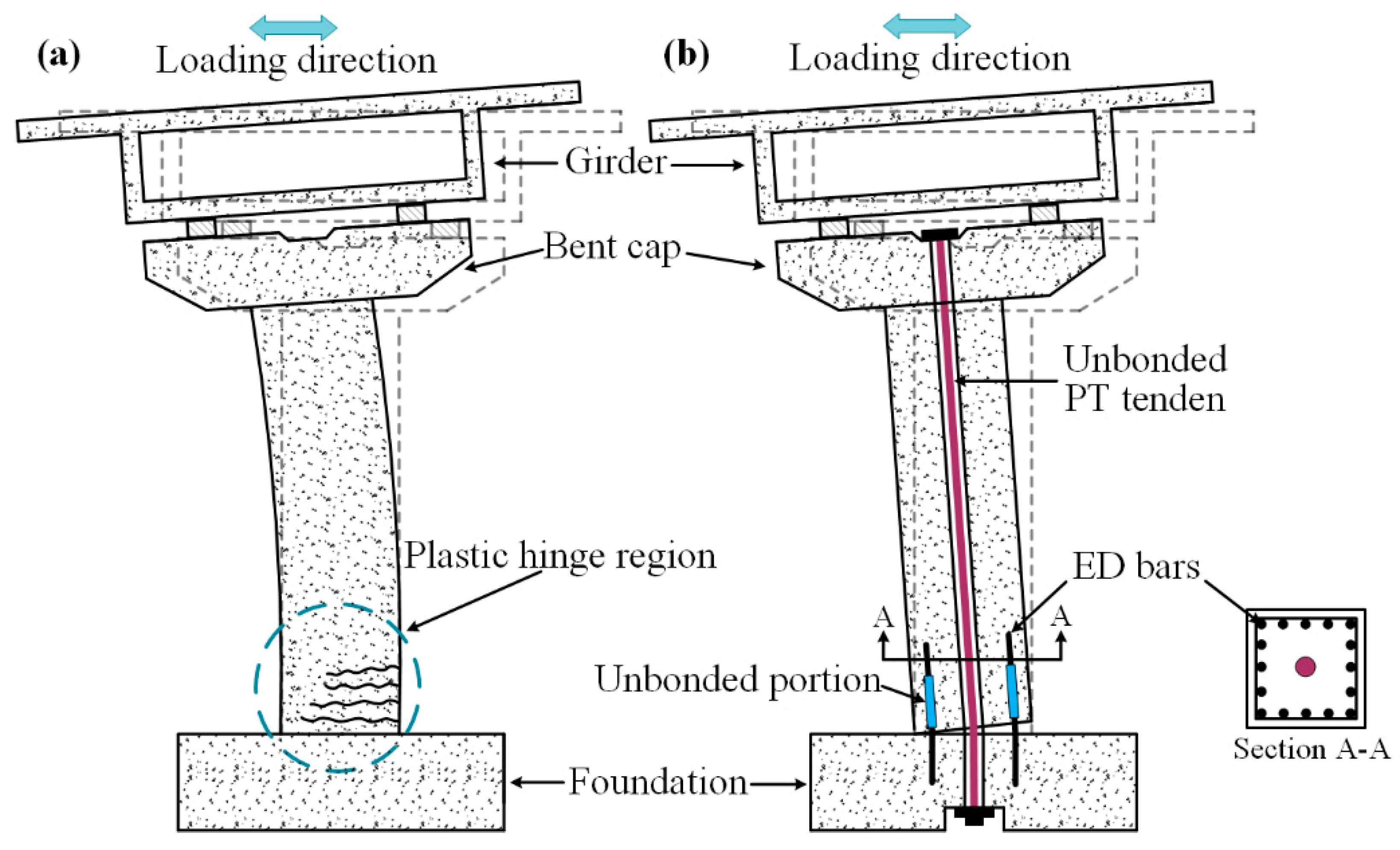
2.1. Description of Laboratory Test Specimens

Based on a series of quasi-static and dynamic tests of the PT rocking pier specimens conducted by Shen et al. [15,22,39,40], four selected numerical models (i.e., LP, MCS-LE, MCS-EP and MCS-NP models) were developed in OpenSees [37]. The specimens in both tests are almost identical in terms of the key dimensions, design parameters, and fundamental material properties. According to Shen et al. [15], the prototype bridge pier is a monolithic single-column circular reinforced concrete (RC) pier, and its design follows the Chinese Specifications TJG/T 2231-01-2020 [41] and JTG B02-2013 [42]. The diameter and height of the prototype pier are 9.5 m and 2.1 m, respectively, and more key properties are summarized in

Table 1. Design parameters of the prototype and the tested specimens.

Design Parameter	Monolithic Prototype	Specimen I	Specimen II
Pier diameter (m)	2.1	0.44	0.44
Pier clear height (m)	8.3	1.75	1.35
Pier effective height (m)	9.5	2.0	2.04
Axial gravity force (kN) [ratio (%)]	7280 [7.5]	323 [7.5]	322.4 [7.5]
initial PT force	—	749 [17.5]	749 [17.5]
Longitudinal reinforcing steel [ratio (%)]	36-D14 [1.32]	6-D16 [0.79]	6-D16 [0.79]
Transverse reinforcing steel [ratio (%)]	D18@80 [0.64]	D8@60 [0.84]	D8@60 [0.84]
PT steel [ratio (%)]	—	1-D40 [0.82]	1-D40 [0.82]
Longitudinal reinforcing + PT steel ratio	1.32	1.61	1.61

.

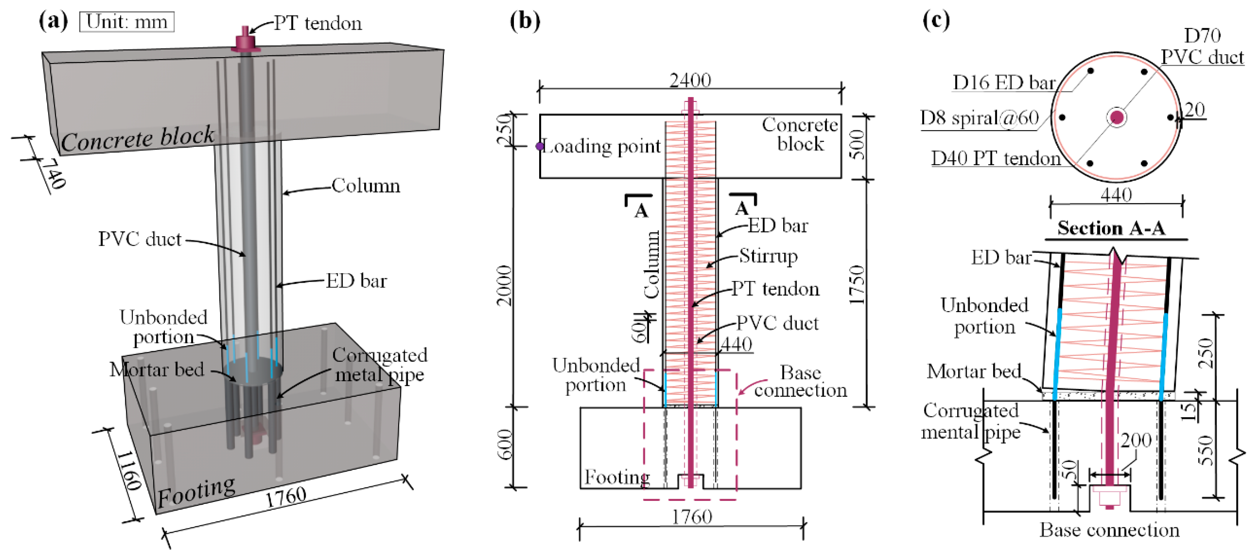
2.1.1. Quasi-Static Test Specimen

Figure 3 depicts the overall dimensions and base detail of the benchmark pier specimen in the quasi-static test (denoted as Specimen I herein) [15]. The scale factor of the specimen (see Figure 3a) for length (S_l) is 1/4.75, resulting in an effective height (from the pier base to the loading point) and sectional diameter (d) of 2.0 and 0.44 m, respectively (Figure 3b). The aspect ratio (the ratio of effective height to cross-sectional depth) of Specimen I is 4.55 and the clear height is designed to be 1.75 m. The axial gravity force (f_G) and the corresponding axial force ratio (α_G) are 323 kN and 7.5%, respectively (see Table 1). One D40 (40 mm in diameter) PT bar [corresponding to a steel ratio (ρ_PT) of 0.82%] is installed to enhance the self-centering behavior. The initial PT force (f_PT) and the corresponding axial force ratio (α_PT) are 749 kN and 17.5%, respectively (see Table 1). Six D16 longitudinal mild bars [corresponding to a steel ratio (ρ_ED) of 0.79%] with an unbonded length(blue line) of 250 mm are designed to enhance the specimen’s ED capacity. Figure 3c shows the cross-section and base details of Specimen I. The thickness of the concrete cover is 20 mm and D8 spiral stirrups (red line) spaced 60 mm apart are designed, which corresponds to a volumetric steel ratio of 0.84%. In addition, a 15 mm thick mortar bed is cast beneath the pier base to level the footing surface and to withstand the high compression stress during rocking as well. Rayleigh damping is used in the modeling process of Specimen I and the damping ratio value is 5%.

The bent cap of Specimen I is downscaled to the dimensions of 2400 × 740 × 500 mm (Figure 3) and the dimensions of the footing are 1760 × 1160 × 600 mm. The detailed design parameters of Specimen I are listed in Table 1. In the quasi-static test, Specimen I was subjected to the identical displacement (drift)-control lateral cycle loading protocol. The loading protocol consisted of 19 cycles of increasing drift levels and was repeated three times. The initial several cycles, which have a drift up to 0.6%, were conducted in an increment of 0.1% to measure the drifts associated with the yielding of the ED bar. Subsequently, the cycles up to 1.6% drift (indicating moderate damage to the pier base) were conducted in an increment of 0.2% drift. The subsequent cycles were conducted in an increment of 0.4% drift until the specimen failed.

2.1.2. Shaking Table Test Specimen

Figure 4 depicts the overall dimensions and base detail of the corresponding specimen in the shaking table test (denoted as Specimen II herein) [40]. For the sake of comparison, the selection and design of Specimen II (see Table 1) are based on the dimension and parameters of Specimen I [40]. The key dimensions, design parameters (e.g., α_G, α_PT, ρ_ED and ρ_PT), and fundamental material properties between the two specimens are nearly identical (see Table 1), except for the steel bracing supports designed in Specimen II (see Figure 4a). Twelve iron blocks are installed on the top of Specimen II to serve as the additional mass. As a result, the center of mass of Specimen II is located at a height of 0.69 m above the column top. To guarantee the same aspect ratio between Specimens I and II, the column’s clear height in Specimen II (see Figure 4b) is shortened to 1.35 m, resulting in an effective height (from the pier base to the center of mass) of 2.04 m, almost identical to that of Specimen I. In addition, a hollow rigid steel support frame is used on the top of the concrete block to keep the unbonded length of the PT bar identical to that in the quasi-static test (i.e., 2.7 m), and a 15 mm thick mortar bed is also designed at the pier base. Rayleigh damping was also used in the modeling process of Specimen II with a damping ratio value of 5%.

The bent cap of Specimen II was downscaled to the dimensions of 2400 × 2400 × 2400 mm (Figure 3) and the dimensions of the footing were 1760 × 1260 × 600 mm. The detailed design parameters and the material properties of Specimen II are also listed in Table 1. In the shaking table test, three earthquake records (El Centro, San Fernando, and Chi-Chi ground motions) were utilized as input motions, and Specimen II was subjected to a loading protocol consisting of three phases: elastic phase, design-basis earthquake phase, and large earthquake phase. Among them, the DBE level tests were selected as the dynamic study cases in this study, and the three ground motion records were scaled to match their acceleration response spectra well with the design spectrum.

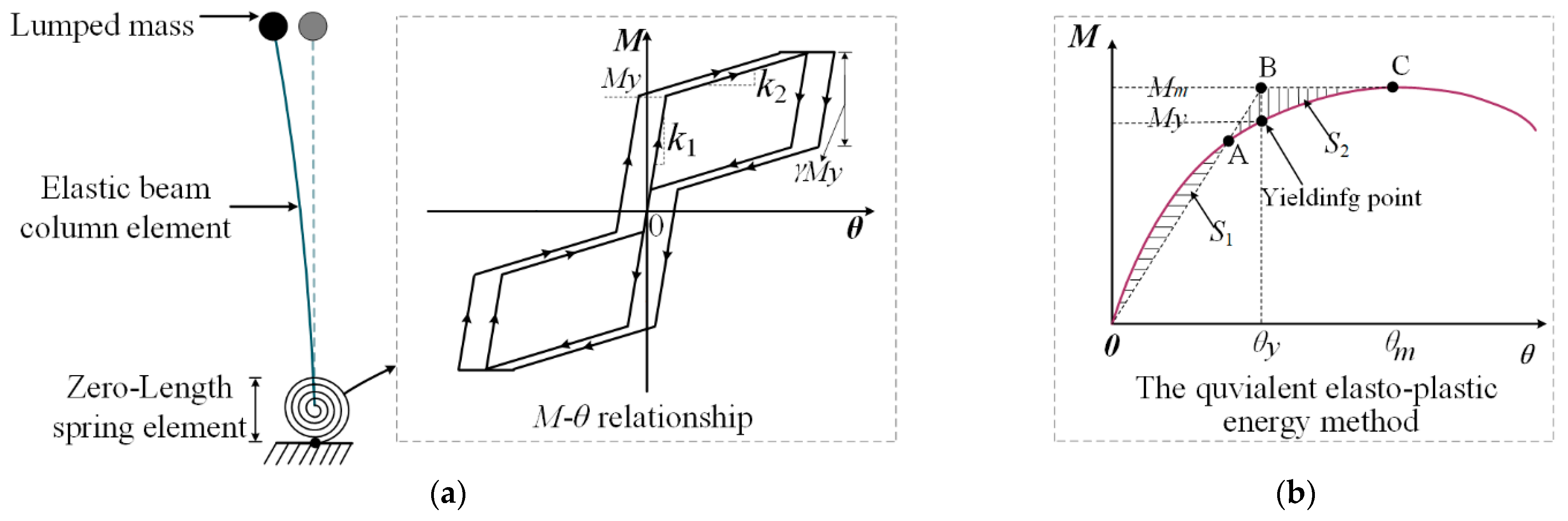
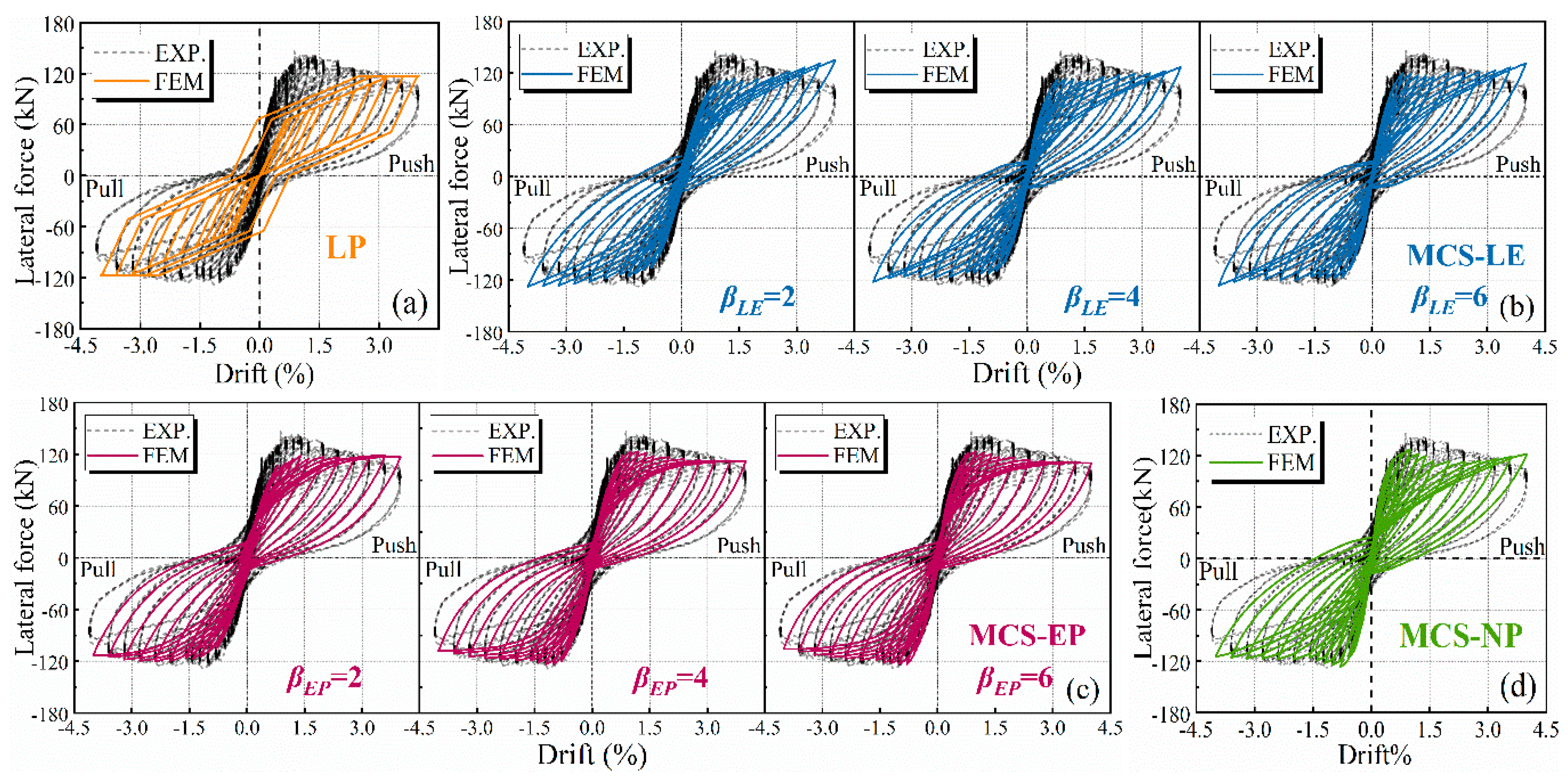
2.2. Lumped Plasticity (LP) Model

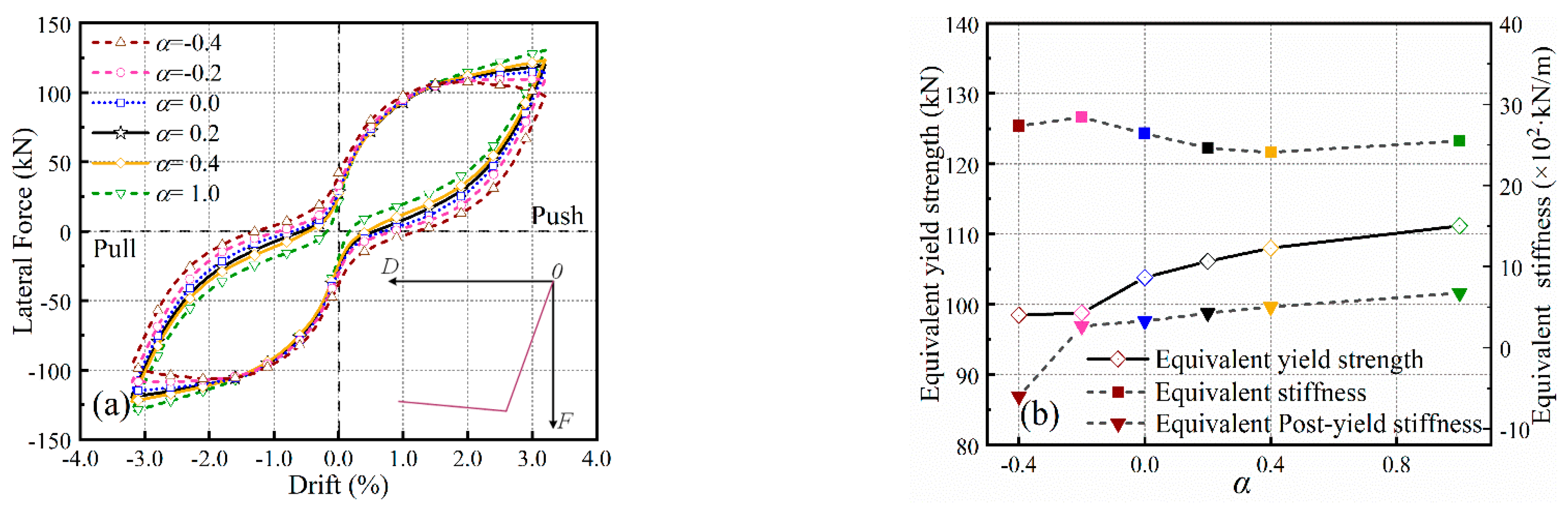
2.2.1. Modeling the Monotonic Behavior

Typically, the moment–rotation (M-θ) relationship of the rotation spring in the LP model is derived from the section analysis approach [14,16]. However, the section analysis approach of PT rocking piers differs from that for conventional monotonic RC piers. In PT rocking piers, an infinite curvature is formed at the base due to the opening and closure of the base interface. Therefore, the M-θ relationship shall be used to define the interface behavior rather than the traditional moment–curvature relationship. At this critical interface, section strain compatibility between the concrete and steel is violated because both PT and ED bars are unbonded/partially unbonded. Pampanin et al. [43] and Palermo et al. [16] developed the “monolithic beam analogy” to resolve the strain incompatibility phenomenon.

2.2.2. Modeling the Cyclic Behavior

The LP model with a single rotational nonlinear spring can be used to simulate rocking behavior [31]. Figure 5a shows a typical LP model for a PT rocking pier. The mass of the PT rocking pier is concentrated at the top of the pier. The pier column is simulated by using an elastic beam column element since it is expected to remain elastic during rocking. A zero-length rotational spring element with “self-centering” material [37] is used to model the base rocking behavior. The M-θ relationship of this single rotational spring is flag-shaped and is depicted in Figure 5 as well, in which M_y is the yield moment; k₁ is the initial stiffness; k₂ is the post-yield stiffness; and γ is the ratio of loading to unloading force. The equivalent elastic–plastic energy method [44,45] is used to estimate the values of M_y, k₁ and k₂ of the column, and its basic principle is shown in Figure 5b, in which the area of S₁ is equal to S₂. In addition, the P-delta effect is included in the model.

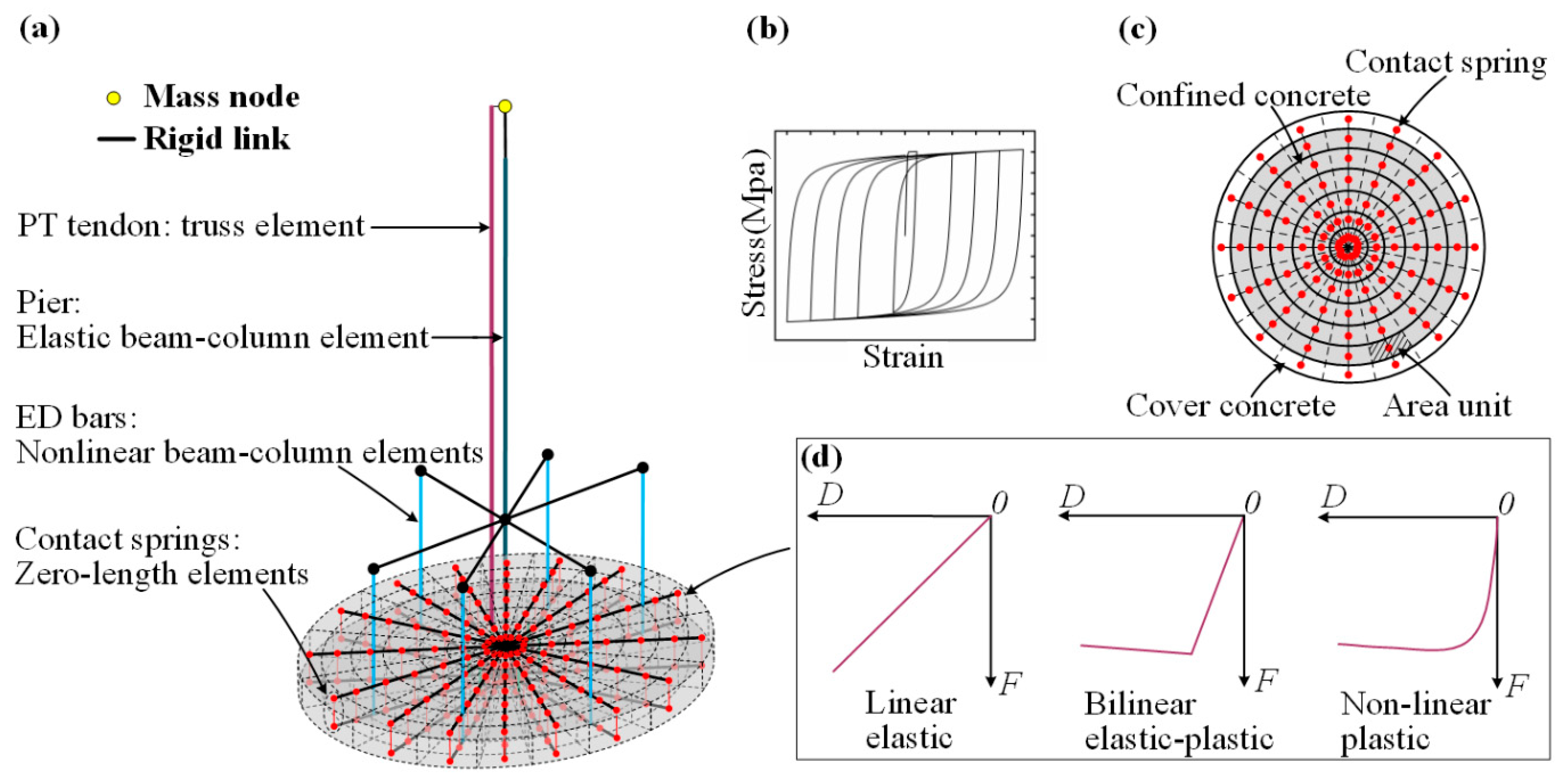
2.3. Multi-Contact Spring (MCS) Model

Figure 6 illustrates the 3D MCS model for a PT rocking pier, in which the rocking interface is modeled by a series of compression-only zero-length spring elements. The pier column is simulated by using an elastic beam column element (see Figure 6a). The PT tendon is modeled by a linear truss element, in which the initial post-tensioning stress is imposed by “Steel 02” material (see Figure 6b), while the ED bars are represented by nonlinear beam column elements with “Steel 02” material as well. It should be noted that the nonlinear properties of “Steel 02” material in the PT bar are excluded via setting a large yielding strength. The pier base is discretized into 7 rings along the radius and 16 segments along the circumference, resulting in a 3D interface with a total of 112 zero-length elements (i.e., area units, see Figure 6c). Each element represents a vertical contact spring and exhibits compression-only behavior. The compression-only F-D relationships for these contact springs (see Figure 6d) are various, which can be set as linear elastic (LE) [23,36], bilinear elastic–plastic (EP) [23,24], and nonlinear plastic (NP) [9,22,35]. Moreover, the P-delta effect is also included in the MCS models. In addition, the bonding effect of ED bars to concrete is also considered in the numerical models. In the cross-section above the unbonded portion of the ED bars, the reinforcement and concrete are well bonded, and thus, the column is modeled by using the fiber section accordingly. However, the bonding effect of ED bars to concrete is damaged due to strain penetration around the unbonded and bonded portion of the ED bars. An equivalent unbonded length (L_eu) is used to represent this phenomenon, which can be determined by Equation (1) suggested by Palermo and Pampanin et al. [33].

$$L_{eu}=0.022d_s{f}_y$$

(1)

where d_s is the diameter of the ED bars, and f_y is the yield strength of the ED bars. Thus, the unbonded length in the ED bars includes two parts: the actual unbonded length (L_ub = 25 cm) and the equivalent unbonded length (L_eu).

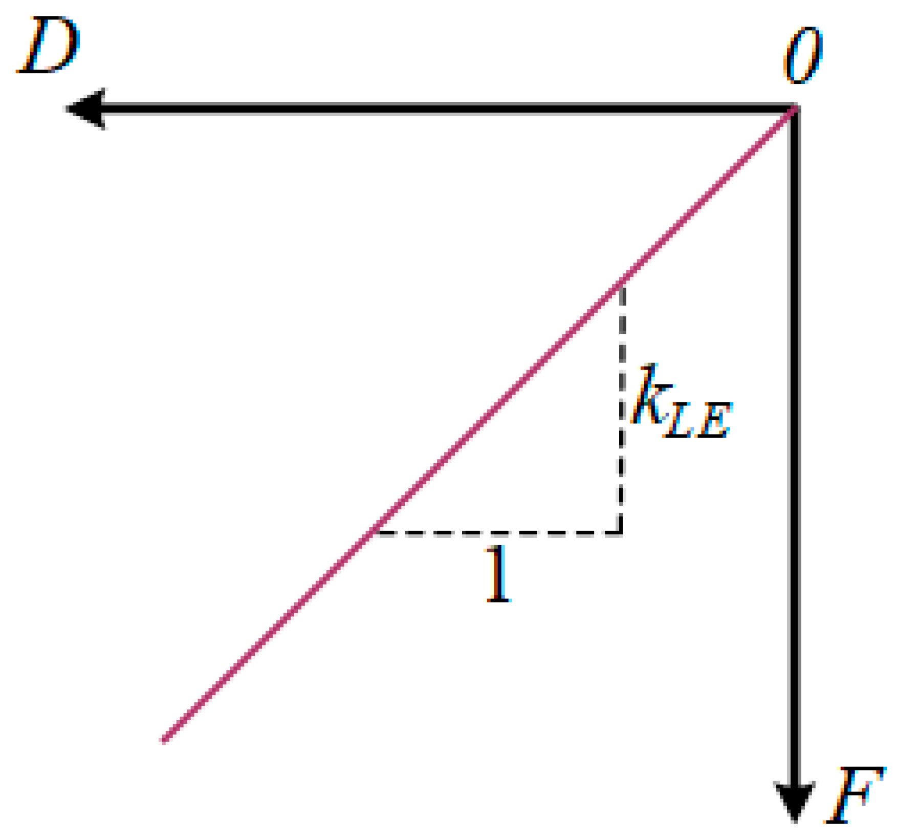
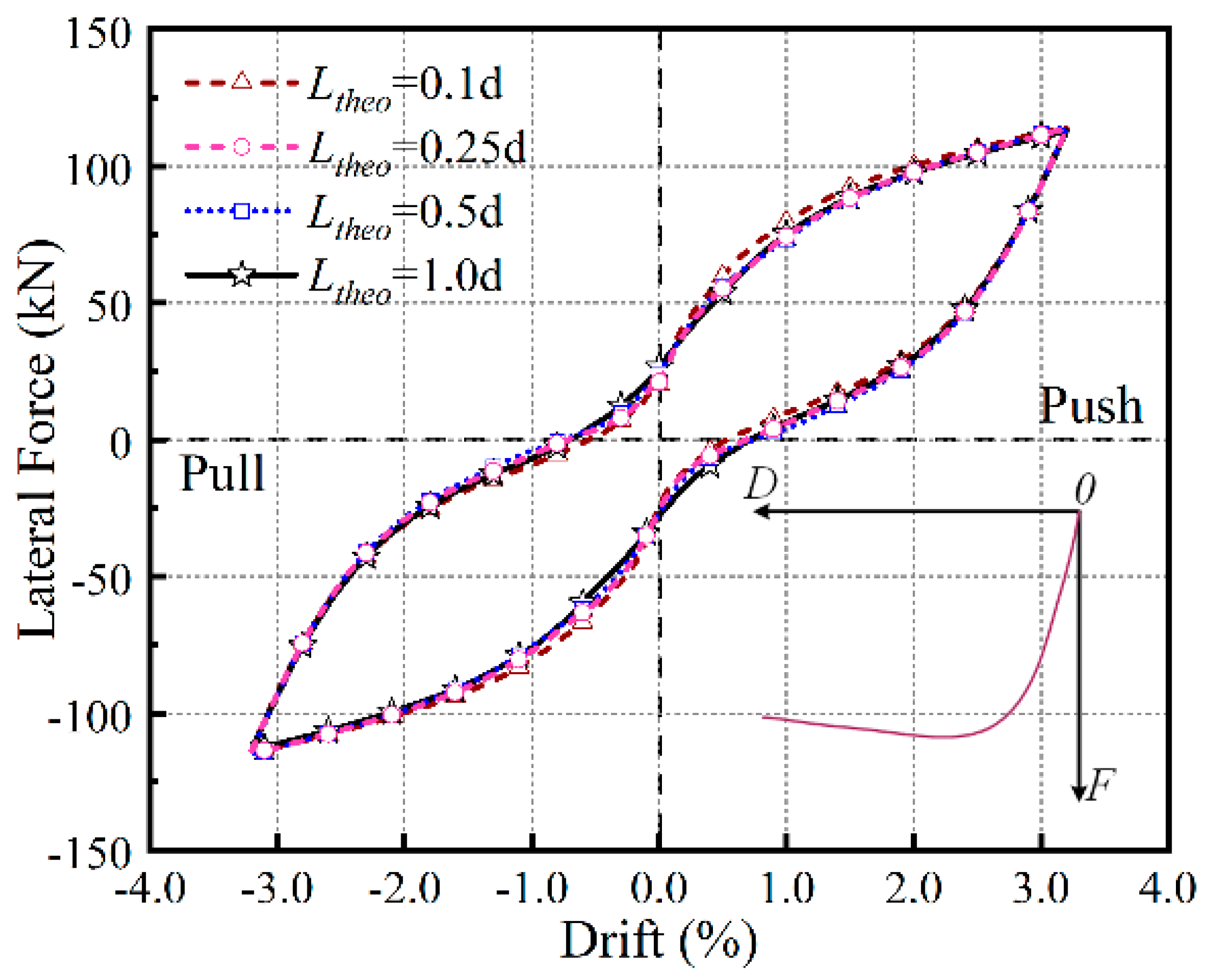
2.3.1. Linear Elastic (LE) Contact Spring

Figure 7 shows the F-D relationship of the MCS-LE model, where k_LE denotes the stiffness of the contact spring. The “linear elastic” material is used to simulate the MCS-LE model. For the 2-dimensional (2D) MCS-LE model, k_LE can be calculated using Equation (2) according to Si et al. [36].

$$k_{LE}=\frac{E_{c}A}{Hm}\beta$$

(2)

where E_c is the elastic modulus of the pier base material, A is the cross-section area of the pier, H is the height of the pier, m is the number of zero-length elements, and β is the modified stiffness factor. Analogically, for the 3D MSC-LE model, this equation can be adjusted by considering the area of each contact element, as follows:

$$k_{LE\_i}=\frac{E_c{A}_i}{H}{\beta }_{LE}$$

(3)

where A_i represents the area of the i-th contact unit area (see Figure 6c); k_{LE_i} represents the stiffness of the i-th contact spring; and β_LE represents the modified stiffness factor for the 3D MSC-LE model.

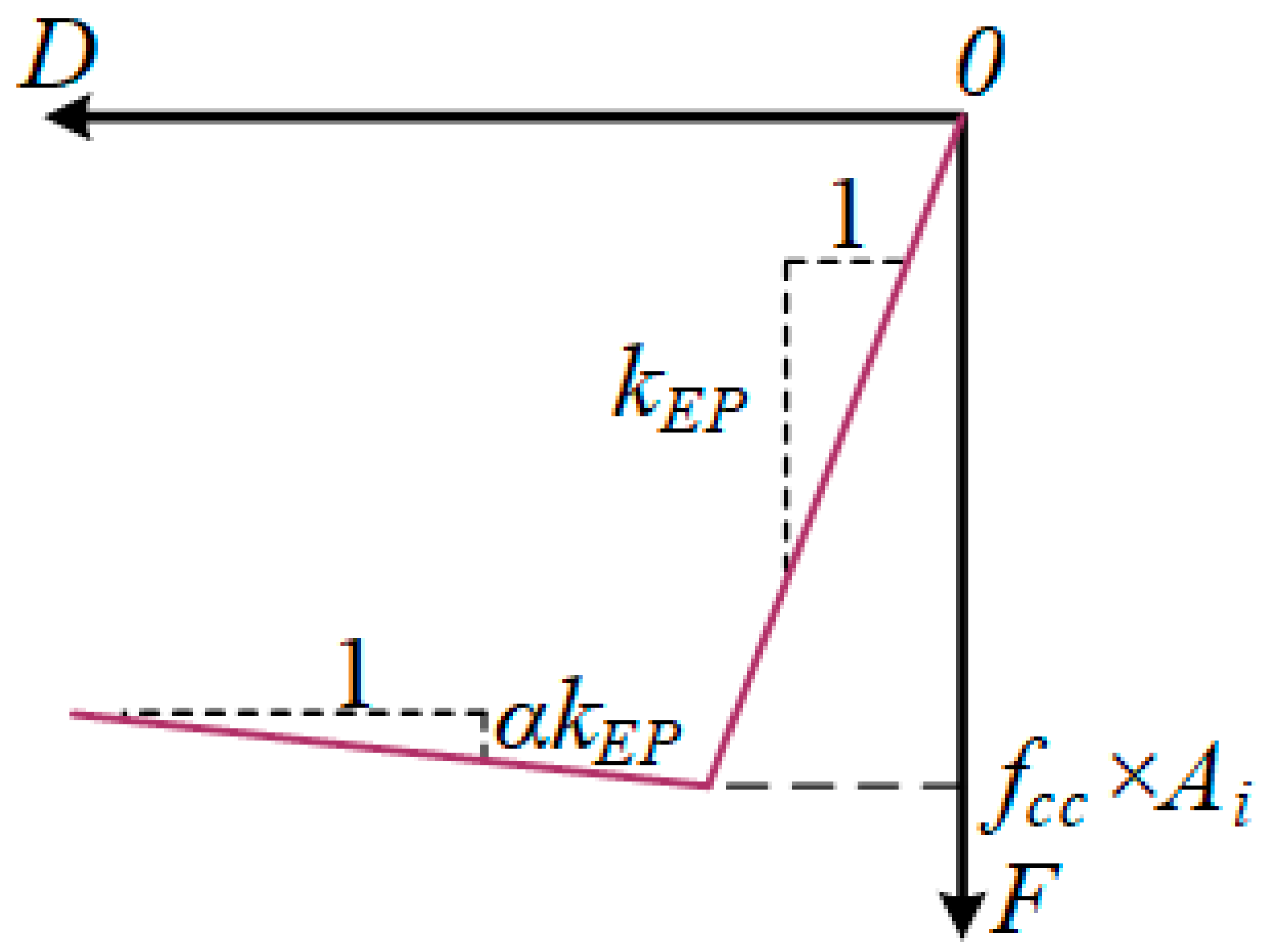
2.3.2. Bilinear Elastic–Plastic Contact (EP) Spring

The bilinear elastic–plastic contact spring (MCS-EP) model, which considers the stiffness degradation due to concrete contact damage, was proposed by Marriott et al. [23,24]. Its elastic stiffness k_{EP_i} can also be determined following Equation (3), but the stiffness modification factor should be changed to be appropriate for the MSC-EP model, i.e., adopting Equation (4).

$$k_{EP\_i}=\frac{E_c{A}_i}{H}{\beta }_{EP}$$

(4)

where β_EP is the modified stiffness factor for the MSC-EP model.

The post-yielding stiffness of the MSC-EP model can be set as αk_{EP_i}; thus, the “Elastic-Perfectly Plastic Gap” material with the gap = 0 is used to simulate the MCS-EP model. Figure 8 shows the typical F-D relationship of the MSC-EP contact spring, which is derived from the stress–strain behavior, where f_cc is the peak strength of the pier base concrete; from the figure, it can be seen that the force of the contact spring is obtained by multiplying the yield stress f_cc by the A_i.

2.3.3. Nonlinear Plastic (NP) Contact Spring

For the MCS-NP model, the behavior of the contact spring is simulated by the “Concrete01” material [9,35], which also needs to be converted into the F-D relationship, as shown in Figure 9. In the F-D relationship, the contact force is related to the contact unit area A_i; while the contact deformation is transformed from the strain (i.e., the peak strain ε_c and ultimate strain ε_u) amplified by the theoretical neutral–axial depth L_theo.

In summary, the LP model with a single rotational nonlinear spring can be used to simulate the rocking behavior of PT rocking piers. However, the hysteretic behavior of the spring is obtained using the section analysis method, which requires an iterative calculation of the neutral axis height c, thereby increasing the computational complexity. The MCS model, utilizing a series of compression-only zero-length springs, can also simulate the rocking behavior of PT rocking piers. In the MCS model, three types of force–displacement (F-D) relationships for these contact springs are used: linear elastic (LE), bilinear elastic–plastic (EP), and nonlinear plastic (NP). However, the contact stiffness parameters of the contact springs (e.g., β_LE and β_EP) in the MCS model usually need to be calibrated using experimental results.

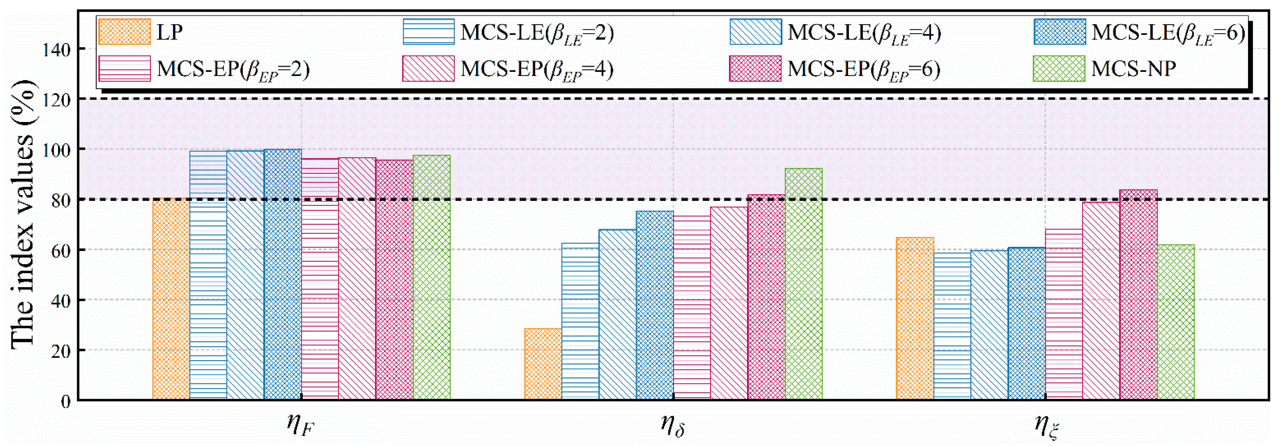
3. Comprehensive Performance Assessment of the MCS Models

Based on the analyses in Section 2.3, it was found that the parameters β_LE, β_EP, α, and L_theo affect the initial stiffness of the contact springs for different F-D relationships of MCS models. To comprehensively investigate their effects on the cyclic behavior of PT rocking piers, a parametric cyclic analysis with a 3.2% target drift using the MCS models, based on Specimen Ⅰ, was conducted and is discussed in the following. Considering that 3.2% is a relatively large excursion during seismic events, it was selected to be the target drift.

3.1. MCS-LE Model

Figure 10a depicts the influence of β_LE on the hysteretic behavior of PT rocking piers using the MCS-LE model, and a more detailed influence on the equivalent yield strength and stiffness (calculated via the equivalent elastic–plastic energy method described in Section 2.2.2) is shown in Figure 10b. It can be seen from Figure 10 that the yield strength and stiffness increased by approximately 40% and 150%, respectively, when the β_LE varied from 0.5 to 8.0, while the pier’s residual deformation was reduced with this increasing range of β_LE; the largest increase in yield strength occurred when β_LE was smaller than 4.0. The yield strength increased by 33.5% when β_LE increased from 0.5 to 4.0; after that, i.e., β_LE = [4.0, 8.0], the yield strength only increased by about 6.0%. Similarly, the equivalent yield stiffness of the pier increased by 125.6% when β_LE increased from 0.5 to 4.0; after that, i.e., β_LE = [4.0, 8.0], the equivalent yield stiffness only increased about 12.9%. Conversely, the pier’s residual drift decreased by 93.7% from 0.95% to 0.06% when β_LE increased from 0.5 to 4.0. Thus, it can be concluded that when β_LE ranges between 0.5 and 4.0, its effect on the cyclic response of PT rocking piers is significant. A larger contact stiffness, i.e., β_LE > 4.0, would have a limited effect on the pier’s cyclic behavior.

3.2. MCS-EP Model

β_EP and α have an important influence on the cyclic response of PT rocking piers in the MCS−EP model. Figure 11 shows the general trend of the effect of these two parameters on the cyclic behavior of PT rocking piers. The variation ranges for β_EP and α are [0.5, 4.0] and [−0.4, 1.0], respectively. Note that the MCS−EP model with a value of α =1.0 is equivalent to the MCS−LE model. Additionally, to enhance clarity and provide a more comprehensive interpretation of the individual effects of β_EP or α, the influences of the single β_EP (i.e., α = 0) and the single α (i.e., β_EP = 2) on the force–drift relationship of the PT rocking pier using the MCS−EP model are presented in Figure 12 and Figure 13, respectively.

Specifically, we set α = 0 and β_EP = 2 as two typical cases to highlight their effect trend. Figure 12a,b, respectively, depict the influence of β_EP (i.e., α = 0) on the force–drift relationship, equivalent yield strength, and stiffness of the PT rocking pier using the MCS-EP model. It can be seen from the figure that the yield strength and stiffness increased by 14.6% and 57.0%, respectively, when the β_EP increased from 0.5 to 8.0, while the variation in β_EP reduced the residual drift of the pier. Note that the majority of the increase in yield strength occurred as the β_EP varied from 0.5 to 4.0; after that, i.e., β_EP = [4.0, 8.0], the yield strength almost remained constant. Similarly, when the β_EP increased from 0.5 to 4.0, the equivalent yield stiffness of the pier increased by 51.2%, while the pier’s residual drift decreased by 37.5%. Thus, it can be concluded that the effect of β_EP on the cyclic response of PT rocking piers is significant when β_EP is between 0.5 and 4.0. Beyond that, the change in β_EP and the resulting contact stiffness variation have a limited effect on the pier’s hysteretic behavior.

Figure 13a, b, respectively, depict the influence of α (i.e., β_EP = 2) on the force–drift relationship, equivalent yield strength, initial stiffness, and post-yield stiffness of the PT rocking pier using the MCS-EP model. It can be seen that a stable positive post-yielding region can be obtained when α ≥ −0.2, and its slope increases with the increase in α, which helps to reduce the residual drift. As shown in Figure 13, when α increases from −0.2 to 1.0, the post-yield stiffness of the pier increases from 264.9 to 672.4 kN/m, while the residual drift reduces from 0.9% to 0.15%.

3.3. MCS-NP Model

According to Section 2.3.3, L_theo is a key parameter to calibrate the force–displacement relationship of the MCS-NP model; thus, four L_theo values (0.10d, 0.25d, 0.5d, and 1.0d) were selected to identify its effect on the hysteretic behavior of the pier. Note that among the four selected values, L_theo = 0.25d is recommended by Guerrini et al. [35]. Figure 14 depicts the effect of L_theo on the lateral force–drift relationship of the PT rocking piers based on the MCS-NP model. Evidently, the hysteresis curves among the four L_theo values are almost identical, indicating that the effect of L_theo on the cyclic response of PT rocking piers is limited. The lateral forces at 3.2% target drift for the cases of 0.1d, 0.25d, 0.5d, and 1.0d are all close to 114 kN, respectively, in the push direction and to 113 kN, respectively, in the pull direction. As a result, L_theo = 0.25d was adopted to calibrate the force–displacement relationship of the MCS-NP model.

In summary, the parameters β_LE, β_EP, and α affect the F-D relationship of MCS models, while the L_theo has a limited effect on the cyclic response of PT rocking piers. The yield strength and stiffness of PT rocking piers increase with the increase in either β_LE or β_EP, while the pier’s residual deformation decreases with the increase in these parameters. The post-yield stiffness of the pier increases with an increase in α, while the residual drift decreases. The effect of α on the equivalent yield strength and initial stiffness is limited.

4. Validation of the Cyclic Responses

The appropriate values of contact parameters (e.g., β_LE and β_EP) are essential for the numerical models to accurately capture the cyclic response of PT rocking piers. In this section, the effectiveness of the four numerical models and their appropriate contact parameter values to reproduce the actual cyclic response of PT piers are evaluated. Specimen I tested under quasi-static loading was selected as the research target, and the recorded test results were used as the comparison benchmark. The drift (displacement)-control lateral cycle protocol is shown in Figure 15, which includes 17 increasing levels (up to 4.0% drift), with each level repeated three times. In addition, the fundamental period of the test specimen is measured as 0.38 s, and the periods of four numerical models are 0.37 s, this being close to the period of the test specimen. It should be noted that the periods of four numerical models are identical because the lateral stiffness of the pier is merely provided by the elastic deformation of the column shaft before rocking.

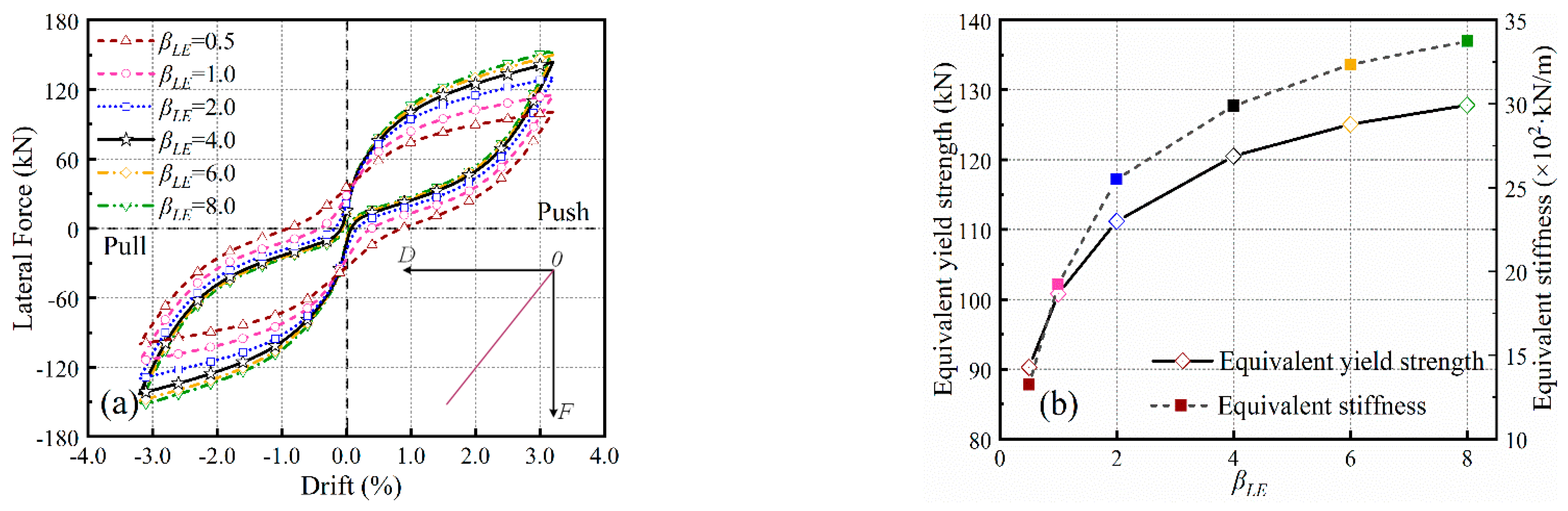
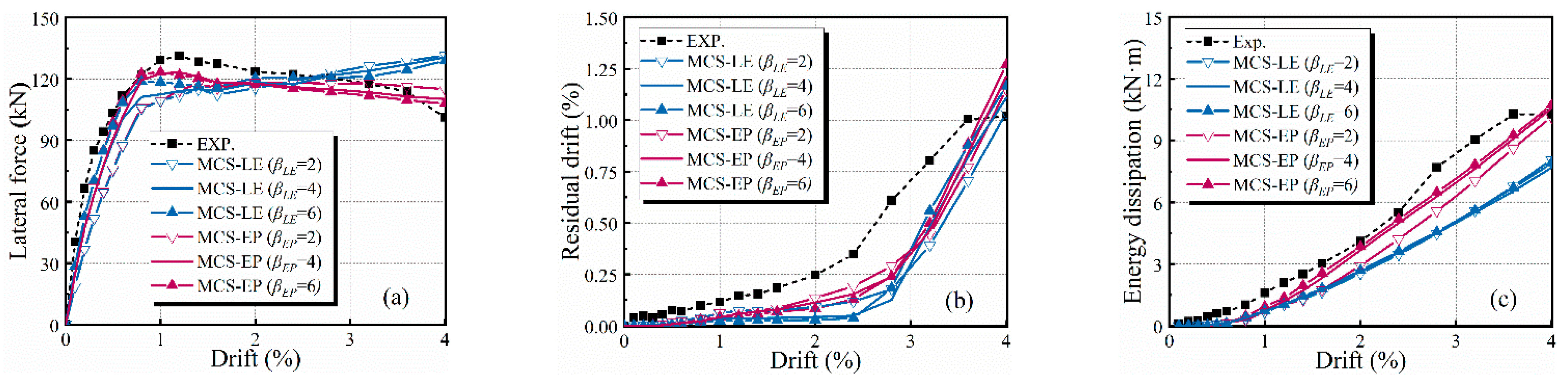
4.1. Force–Drift Relationship

Figure 16 shows a comparison between the simulation and test results for the force–drift hysteretic response of the four contact models. In general, good agreement was achieved between the test data and the numerical results produced by the various models for PT rocking piers in terms of the hysteretic responses, e.g., initial stiffness, post-yield stiffness, yield strength, and residual drift. However, some small differences between the experimental and numerical force capacity between the pull and push directions can be observed. This is due to the inhomogeneity of the concrete material and construction tolerances, resulting in an asymmetry in the force capacity of Specimen I. Thus, the average results in the push and pull directions were used for the following detailed comparison.

Using the LP model, a lower initial stiffness was observed compared to the test results, as shown in Figure 16a. This is attributed to the simplification of the M-θ relationship obtained by the section analysis approach for the LP model, and thus, the LP model would underestimate the lateral force of the PT rocking pier when the drift is less than 3.0%. At large drifts (i.e., > 3.0%), the LP model exhibits a relatively accurate representation of the lateral force for the PT rocking pier. In addition, the residual deformation between the LP model simulation and experimental results also has a good match. At 4.0% drift, the average residual drift calculated by the LP model is 0.8%, this being close to that reordered in the tests (i.e., 1.0%).

A similar comparison is also presented for the hysteretic response of the three MCS models, as shown in Figure 16b, d. Note that for the MCS-LE and MCS-EP models, the simulation results are given for three stiffness modification factor values of 2, 4, and 6, since all of them are close to the experimental data. It can be seen that the results in all these MCS cases show good agreement between the experimental and numerical results in terms of hysteretic responses. This means that the range of [2,6] is appropriate for both β_LE in the MCS-LE model and β_EP in the MCS-EP model. However, it is worth mentioning that, differing from the MCS-EP and MCS-NP models, which consider a degradation of the contact spring stiffness (i.e., smaller post-yielding contact stiffness), the constant contact stiffness in the MCS-LE model leads to an increasing trend in the lateral force, and thus, it exhibits a greater force than the experimental results, especially when the drift exceeds 3.0%.

To better understand the difference between these four models, Figure 17 shows further comparison results of the envelopes for the force–drift relationships between the experimental and simulation data. As mentioned before, the results are the average envelopes in the push and pull directions. Stiffness modification factor values of 4 were used for MCS-LE and MCS-EP models in the comparison of different models. It can be seen from Figure 17 that all models can effectively predict the average backbone curves, except for the LP model, which underestimates the specimen’s lateral force before 3% drift because of the essential assumptions on the M-θ relationship. In addition, among the three MCS models, the MCS-NP exhibits a slightly larger initial stiffness than the MCS-LE and MCS-EP models due to the smaller β_EP value used, but their peak load capacity that approximately occurs at 1.0% drift is still comparable.

4.2. Residual Drift and Energy Dissipation (ED)

The residual drift and energy dissipation comparison results between the test and numerical simulation with four contact spring models are shown in Figure 18. Stiffness modification factor values of 4 were also used for MCS-LE and MCS-EP models as an example. As shown in Figure 18a, there is a discrepancy in residual displacements between the numerical and experimental results. This is due to the lack of consideration for prestress losses during the simulation process. Also, the material constitutive models used in OpenSees may not totally represent the actual material properties. However, the residual displacements observed in both the numerical and experimental results are small, both in accordance with the characteristics of PT rocking piers. Furthermore, all contact spring models generally underestimate the pier’s residual drift as a result of the pier column elastic simulation. In fact, there existed some spalling of the concrete cover around the pier base during the cyclic testing of Specimen I, especially after the drift of 2.4%, which contributed to the increase in the residual deformation. More specifically, at a drift of 2.4%, the MCS-LE, MCS-EP, and MCS-NP models predict residual drifts of 0.05%, 0.15%, and 0.17%, respectively, which are 85.9%, 55.8%, and 51.1% lower than the test results; as for the LP model, it produces almost no residual drift when the 2.4% drift is applied (i.e., having the largest difference compared to the test results), and the obvious residual deformation can be observed only after 3.2% drift. This phenomenon of underestimating the residual deformation would gradually be suppressed at large drifts. At 4.0% drift, the differences between the simulation and test results for the MCS-LE, MCS-EP, and MCS-NP models decrease to only 8.9%, 19.1%, and 24.9%, respectively; however, as expected, the LP contact model still has the modest difference due to its simplification.

The energy dissipation comparison results between the test and numerical simulation with four contact spring models are shown in Figure 18b. It can be seen from Figure 18b that, in general, all models underestimate the energy dissipation of the pier as well, with the MCS-EP model showing relatively superior prediction results compared to the other models. At 4.0% drift, the difference between the simulation and test results for the MCS-EP model is only 2.7%, while that for the MCS-LE, MCS-NP, and LP models is 25.3%, 21.5%, and 14.9%, respectively. In addition, note that at large drifts, the energy dissipation amount simulated by the LP model has a sharp increase trend, and at 4.0% drift, it even exceeds the test results. This is because the ‘self-centering’ material (see Figure 5) used in the LP model neglects the effect of degraded reloading stiffness during cyclic loading, which would overestimate the area of the force–drift curves (i.e., energy dissipation capacity).

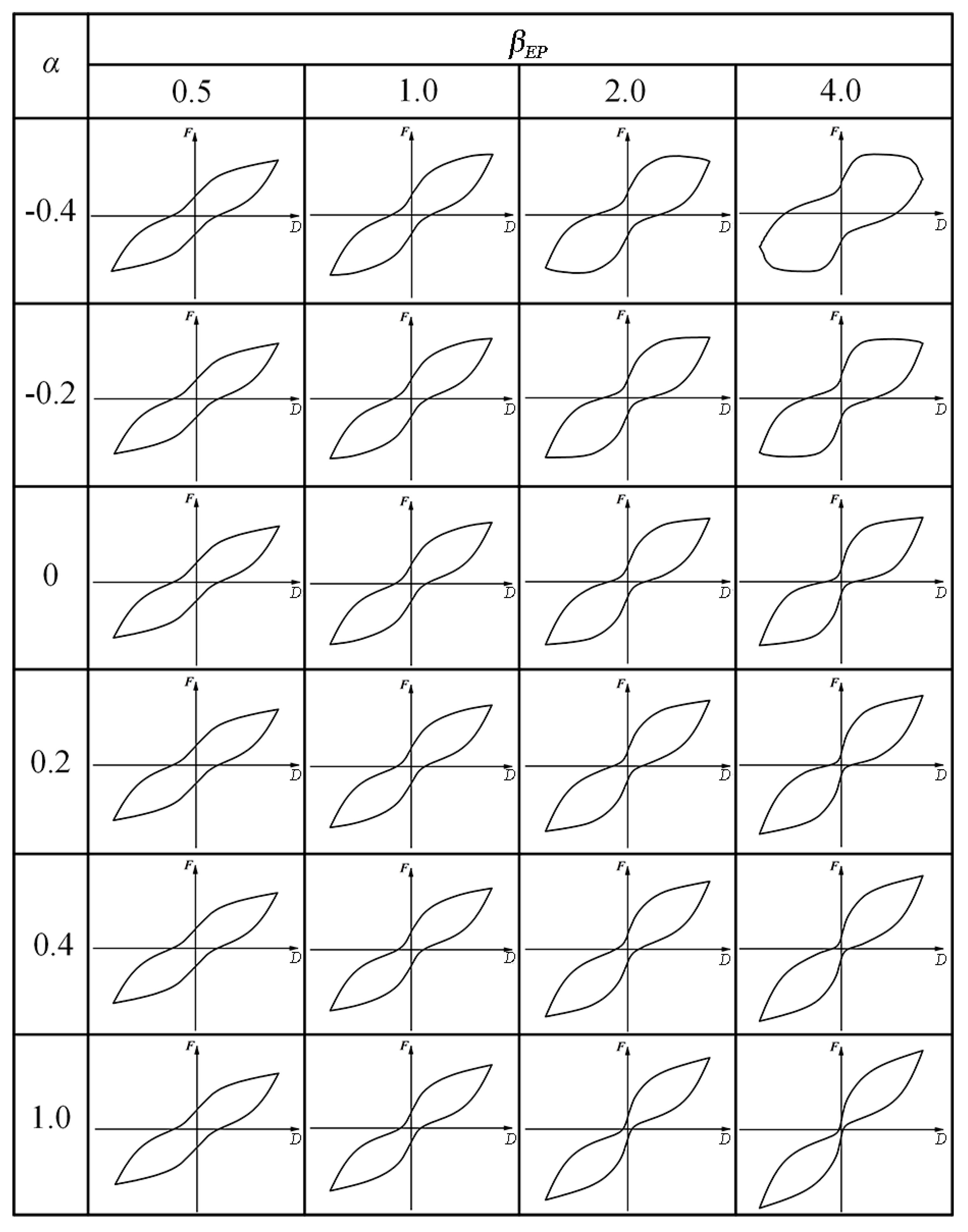
4.3. Insight into the Modified Stiffness Factor

As mentioned before, the modified stiffness factors of 2, 4, and 6 are all suitable for the MCS-LE and MCS-EP models to reproduce the pier’s cyclic behavior. To comprehensively evaluate the difference in various cyclic responses when the modified stiffness factors (i.e., β_LE and β_EP) change within the range of [2,6], Figure 19 compares the average envelope, residual drift, and ED results of the MCS-LE and MCS-EP models under these three typical values. Additionally, the corresponding test results are also provided in the figure to give a clear comparison. It can be seen that, as expected, the three cyclic responses derived from the force–drift curves when β_LE and β_EP are set as 2, 4, and 6 are similar, and all the results are close to the corresponding test results. The small difference among the responses under three factor values is related to the contact stiffness and the resulting elastic stiffness of the pier. As shown in Figure 19a, a slightly larger elastic stiffness of the pier can be observed for the cases of β_LE = 6 and β_EP = 6 compared to the other two smaller factor values. However, in the MCS-LE and MCS-EP models, this larger elastic stiffness of the pier does not significantly affect the peak lateral force, residual deformation (see Figure 19b), or ED capacity (see Figure 19c). Moreover, it can be seen from Figure 19b that the numerical results are slightly lower than the experimental results. The difference between the numerical and experimental results is due to the prestress loss of the PT bar in the experiment. The preforce loss in the experiment is related to the concrete spalling and the consequent column’s shortening. Also, the anchorage seating loss in the end anchors of the PT bar during loading could have contributed to the PT force loss.

4.4. Validation Evaluation

For a quantitative evaluation of the effectiveness of four contact spring models to predict the cyclic responses of the PT rocking pier, three response evaluation indexes are proposed: lateral force index η_F, residual drift index η_δ, and ED index η_ξ. These three dimensionless index parameters can be defined as follows:

$${\eta }_i=\frac{1}{n}{\displaystyle \sum _{j=1}^n\frac{ed{p}_{i\_j}}{ED{P}_{i\_j}}}$$

(5)

where edp_{i_j} and EDP_{i_j} are the i-th engineering demand, such as the lateral force, residual drift, and energy dissipated amount, at the j-th drift of the numerical and test results, respectively; n is the number of the evaluated drift levels.

Figure 20 shows the specific values of η_F, η_δ, and η_ξ under various contact spring models. In this study, the acceptable range of the evaluation indexes was set as 0.8~1.2. Within this range, the model is considered able to accurately predict the cyclic behavior of the PT rocking pier. From the figure, it can be seen that, from the viewpoint of the force, the four contact spring models all have the satisfied prediction capacity, and the η_F of the MCS-LE model with β_LE between 2 and 6 is even almost equal to 1.0. However, in terms of predicting the residual drift, only the MCS-EP model with β_EP = 6 and the MCS-NP model can keep the value of the index η_δ within the range of [0.8, 1.2]. Specifically, the η_δ value for the MCS-EP model with β_EP = 6 is 0.82, and for the MCS-NP model, it is 0.92. Conversely, the η_δ value of the LP model is less than 0.4, again quantitatively highlighting the deficiency of this model in predicting the residual state of a PT rocking pier. In addition, simulating the ED of the pier using four contact spring models is not satisfactory based on the proposed evaluation index and range. Only the MCS-EP model with β_EP = 6 exhibits a value of η_ξ of approximately 0.84, which is within the range of 0.8 to 1.2. The second highest η_ξ value is from the MCS-EP model with β_EP = 4, but its value is 0.79, which is not within the 0.8 to 1.2 range. Consequently, among various contact spring models, only the simulation results of the MCS-EP model with β_EP = 6 can meet the satisfactory range of all evaluation indexes.

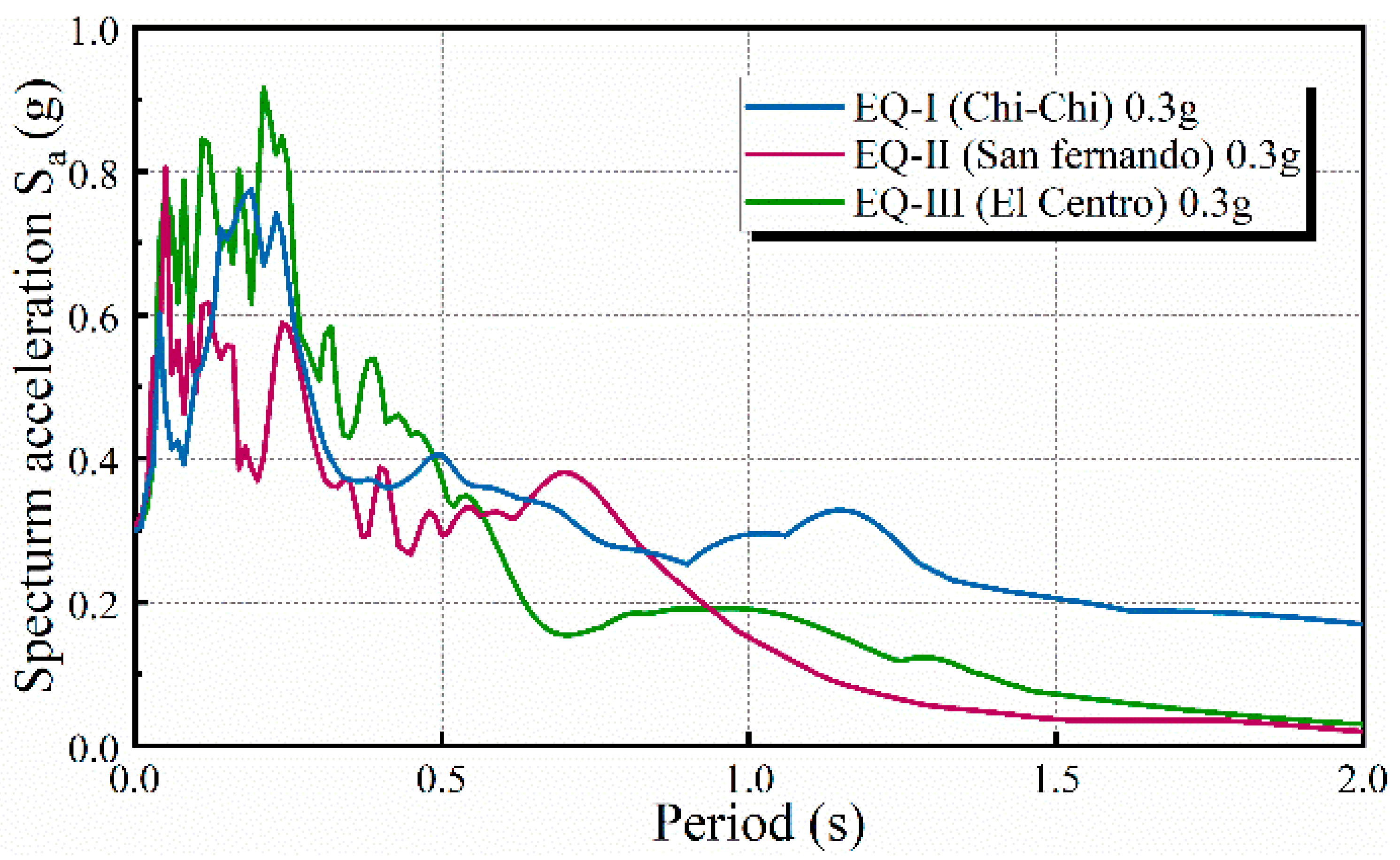
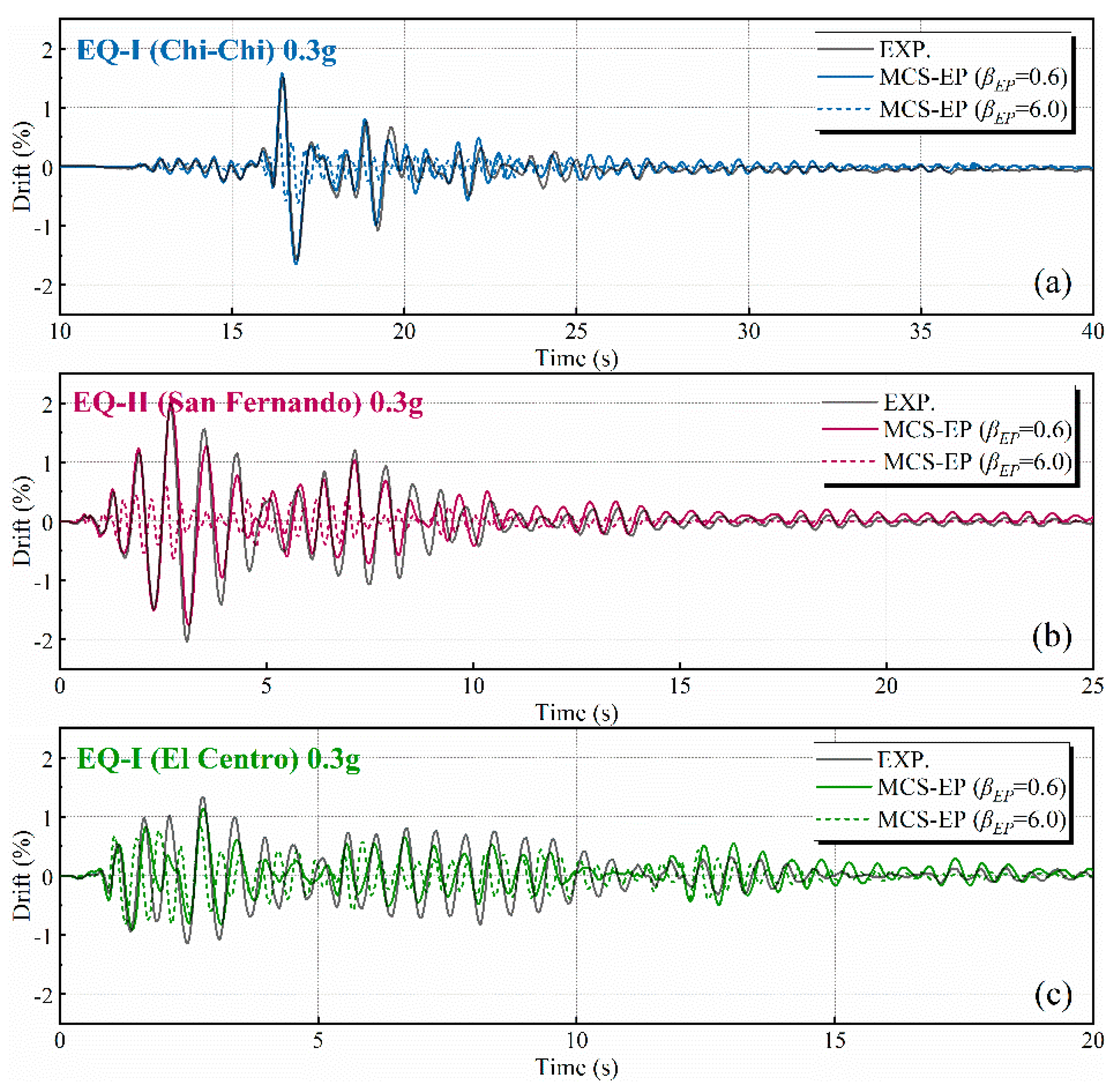
5. Comparison with Shaking Table Testing Responses

Based on the analysis in Section 4, the MCS-EP model is a relatively better option among the four contact spring models for predicting the cyclic behavior of PT rocking piers in terms of force and residual drift, and it also includes the stiffness modification factor β_EP, which can be used to adjust the contact states. Thus, this contact spring model was used to further reproduce the seismic behavior of the pier (i.e., Specimen II) in the shaking table tests. The peak and residual drifts were set as the key comparison responses, and the spring stiffness values of the MEC-EP model used for the dynamic analysis are discussed here.

5.1. Input Ground Motions

Three horizontally recorded ground motions in the shaking table tests [32] were used as inputs for the seismic evaluation in numerical simulations. The ground motions were consistent with the design response spectrum and were scaled to 0.3 g. Figure 21 and Figure 22 show the acceleration time histories and response spectra of the ground motions with a peak ground acceleration (PGA) of 0.3 g, respectively. These three ground motions are, respectively, the 1999 Chi-Chi, 1971 San Fernando, and 1940 Imperial Valley (El Centro station) earthquakes. More details of these ground motions are given in Shen et al. [40]. Moreover, the predominant period of the input motion is 0.32 s, which is closed to the fundamental period of the test specimen.

5.2. Nonlinear History Results

During the preliminary numerical comparison, an obvious difference was observed between the simulation results of β_EP = 6 and the dynamic test data. Thus, the β_EP was adjusted moderately, and it was found that a good match was achieved (i.e., peak and residual drifts) when a smaller value of β_EP (i.e., β_EP = 0.4 to 0.6) was selected. Thus, the contact stiffness used for quasi-static and dynamic analysis is different, which is expected because the contact state is different between the static and dynamic rocking interface. Herein, β_EP = 6 was defined as the static stiffness of the contact spring, while β_EP = 0.4 to 0.6 was used for the dynamic stiffness of the contact spring (i.e., the dynamic stiffness was between 1/15 and 1/10 of the static stiffness).

The time history drift results of the numerical models with β_EP = 6 and 0.6, together with the test results, were plotted as an illustration example. Figure 23 shows the time history responses of the test (solid black line) and numerical results using the MCE-EP model (static stiffness β_EP = 6: the colored dashed line; dynamic stiffness β_EP = 0.6: colored solid line) under the selected three seismic excitations. It can be seen that, compared to the simulation results calculated with static stiffness, the results with the dynamic stiffness match the test results well. Figure 24 provides the specific values of the peak drift for the history response, and the error between the test and simulation is also shown in the figure. The maximum peak drift errors estimated using the MCS-EP model with static stiffness are 59.5%, 67.6%, and 35.3% for EQ-I, EQ-II, and EQ-III, respectively, while the corresponding errors for the dynamic stiffness are reduced to only 14.3%, 0.5%, and 5.1%, respectively. In fact, under dynamic loading, the contact at the rocking interface is related to the inertial effect, and instantaneous impact occurs, which is neglected under cyclic loading. Thus, relying solely on the contact stiffness obtained from quasi-static testing to reproduce the seismic behavior of PT rocking piers is insufficient, and the dynamic contact stiffness can be further developed by multiplying a reduction factor. In addition, due to the self-centering property of the PT rocking pier, very small residual drifts are observed, and the difference between the test and numerical results can be neglected accordingly.

PT rocking piers have garnered widespread attention due to their excellent self-resetting and low-damage capabilities [46,47]. As discussed in this section, a shaking table test of a typical PT rocking pier was adopted to calibrate and validate the MCS-EP model. The MCS-EP model can predict the pier’s seismic behavior after calibrating the contact spring stiffness values, showing good agreement with the test results for the specimens. Additionally, the suggested values of the model spring stiffness for both dynamic and quasi-static analyses were identified through parametric analysis. The recommended contact stiffness for the dynamic analysis of PT rocking piers is smaller than that for the quasi-static analysis. This study validates the 3D contact stiffness equation for the MCS-EP model and assesses the differences between the dynamic and static stiffness values of the contact springs. Furthermore, the results and findings provide a valuable reference and solution for the numerical simulation of PT rocking piers.

6. Conclusions

This paper numerically investigates four common contact spring models to simulate the cyclic and seismic responses of PT rocking piers. There are, respectively, the lumped plasticity (LP) model and multi-contact spring (MCS) models with linear elastic (MCS-LE), bilinear elastic–plastic (MCS-EP), and nonlinear plastic (MCS-NP) material properties. Based on the quasi-static and shaking table tests conducted by the authors, the stiffness values of all contact models that can reproduce the pier’s cyclic and seismic responses are identified, and their simulation results are compared. The main findings and conclusions can be summarized as follows:

(1) All four commonly used spring contact models can predict the cyclic response of PT rocking piers. However, the MCS contact models have a better prediction capacity than the LP contact model. Specifically, for small drifts (i.e., drift < 3.0%) during cyclic loading, the LP model exhibits lower elastic stiffness compared to test data, resulting in an underestimation of the pier’s lateral force. In contrast, the three MCS models show better agreement with the test results. Among the three MCS models (i.e., the MCS-LE, MCS-EP, and MCS-NP), the MCS-EP model is considered the best simulation option based on the developed evaluation indexes. In general, the LP model is a better choice when high computational accuracy is not required. The MCS-EP model should be used when high computational accuracy is essential. The MCS-LE and MCS-NP models provide a balanced approach, offering a compromise between computational time and simulation accuracy.

(2) Simplified contact stiffness equations for the 3D rocking surface of the MCS-LE and MCS-EP models are developed by analogy with the contact stiffness in traditional structural pounding. In the developed equations, the modified stiffness factors β_LE and β_EP are used to calibrate the contact state. Based on quasi-static test results, a value of 6.0 is recommended for cyclic analysis.

(3) Due to the potential instantaneous contact at the rocking interface under dynamic loading, together with the effects of friction and inertia, the spring stiffness used to simulate the seismic behavior of PT rocking piers is different from that of the quasi-static scenario. Typically, the spring stiffness of the MCS-EP model for the dynamic analysis is only about 1/15 to 1/10 of that for the quasi-static contact stiffness; i.e., the β_EP used for the dynamic analysis can be set as 0.4 to 0.6.

(4) Considering the complexity and uncertainty of the rocking motion at the PT pier base under external excitations, the simulation of the contact motion needs to consider the characteristics of the excitation (e.g., static, impulse, or dynamic). Thus, to accurately reproduce the seismic response of PT rocking piers under dynamic excitation, more shaking table studies are needed to investigate the contact state rather than only quasi-static tests (the lack of inertial effect). Moreover, in the numerical modeling of PT rocking piers, it is recommended to consider the impact of prestress loss. Additionally, cumulative damage should also be taken into account in material constitutive models.

References

1. Xia, X.; Zhang, X.; Shi, J.; Tang, J. Seismic isolation of railway bridges using a self-centering pier. Smart Struct. Syst. 2021, 27, 447–455. [Google Scholar]
2. Xu, W.; Ma, B.; Duan, X.; Li, J. Experimental investigation of seismic behavior of UHPC connection between precast columns and footings in bridges. Eng. Struct. 2021, 2390, 112344. [Google Scholar] [CrossRef]
3. Littleton, P.; Mallela, J. Iowa Demonstration Project: Accelerated Bridge Construction on US 6 Over Keg Creek; Department of Transportation, Faderal Highway Administration: Washington, DC, USA, 2013. [Google Scholar]
4. Kagioglou, P.; Katakalos, K.; Mitoulis, S. Resilient connection for accelerated bridge constructions. Structures 2023, 33, 3025–3039. [Google Scholar] [CrossRef]
5. Cao, L.; Li, C. A high performance hybrid passive base-isolated system. Struct. Control Health Monit. 2023, 29, e2887.1–e2887.26. [Google Scholar] [CrossRef]
6. Li, C.; Chang, K.; Cao, L.; Hang, Y. Performance of a nonlinear hybrid base isolation system under the ground motions. Soil Dyn. Earthq. Eng. 2021, 143, 106589.1–106589.15. [Google Scholar] [CrossRef]
7. Guo, A.; Gao, H. Seismic Behavior of Posttensioned Concrete Bridge Piers with External Viscoelastic Dampers. Shock Vib. 2016, 2016, 1823015.1–1823015.12. [Google Scholar] [CrossRef]
8. Chen, X.; Xia, X.; Zhang, X.; Gao, J. Seismic performance and design of bridge piers with rocking isolation. Struct. Eng. Mech. 2020, 73, 447–454. [Google Scholar]
9. Li, Y.; Li, J.J.; Shen, Y. Quasi-static and nonlinear time-history analyses of post-tensioned bridge rocking piers with internal ED bars. Structures 2021, 32, 1455–1468. [Google Scholar] [CrossRef]
10. Wakjira, T.; Rahmzadeh, A.; Alam, M.; Tremblay, R. Explainable machine learning based efficient prediction tool for lateral cyclic response of post-tensioned base rocking steel bridge piers. Structures 2022, 44, 947–964. [Google Scholar] [CrossRef]
11. Shi, X.; Song, L.; Guo, T.; Pan, Z. Seismic design of self-centering bridge piers considering soil-structure interaction. Structures 2022, 43, 1819–1833. [Google Scholar] [CrossRef]
12. Priestley, M.J.N.; Sritharan, S.; Conley, J.R.; Pampanin, S. Preliminary Results and Conclusions From the PRESSS Five-Story Precast Concrete Test Building. PCI J. 1999, 44, 42–67. [Google Scholar] [CrossRef]
13. Kwan, W. Unbonded posttensioned concrete bridge piers, I: Monotonic and cyclic analyses. J. Bridge Eng. 2003, 8, 92–101. [Google Scholar] [CrossRef]
14. Roh, H.; Ou, Y.; Kim, J.; Kim, W. Effect of yielding level and post-yielding stiffness ratio of ED bars on seismic performance of PT rocking bridge piers. Eng. Struct. 2014, 81, 454–463. [Google Scholar] [CrossRef]
15. Shen, Y.; Freddi, F.; Li, Y.; Li, J. Parametric experimental investigation of unbonded post-tensioned reinforced concrete bridge piers under cyclic loading. Earthq. Eng. Struct. Dyn. 2022, 51, 3479–3504. [Google Scholar] [CrossRef]
16. Palermo, A.; Pampanin, S.; Marriott, D. Design, modeling, and experimental response of seismic resistant bridge piers with posttensioned dissipating connections. J. Struct. Eng. 2007, 133, 1648–1661. [Google Scholar] [CrossRef]
17. Xu, F.; Zhang, X.; Xia, X.; Shi, J. Study on seismic behavior of a self-centering railway bridge pier with sacrificial components. Structures 2022, 35, 958–967. [Google Scholar] [CrossRef]
18. Zhao, J.; Wu, B.; Ou, J. A novel type of angle steel buckling-restrained brace: Cyclic behavior and failure mechanism. Earthq. Eng. Struct. Dyn. 2011, 40, 1083–1102. [Google Scholar] [CrossRef]
19. Roh, H.; Reinhorn, A. Hysteretic behavior of precast segmental bridge piers with superelastic shape memory alloy bars. Eng. Struct. 2010, 32, 3394–3403. [Google Scholar] [CrossRef]
20. Govahi; Ehsan; Salkhordeh, M.; Mirtaheri, M. Cyclic performance of different mitigation strategies proposed for segmental precast bridge piers. Structures 2022, 36, 344–357. [Google Scholar] [CrossRef]
21. Salkhordeh; Govahi, E.; Mirtaheri, M. Seismic fragility evaluation of various mitigation strategies proposed for bridge piers. Structures 2021, 33, 1892–1905. [Google Scholar] [CrossRef]
22. Shen, Y.; Freddi, F.; Li, J. Experimental and numerical investigations of the seismic behavior of socket and hybrid connections for PCFT bridge columns. Eng. Struct. 2022, 253, 113833. [Google Scholar] [CrossRef]
23. Marriott, D.; Pampanin, S.; Palermo, A. Quasi-static and pseudo-dynamic testing of unbonded post-tensioned rocking bridge piers with external replaceable dissipaters. Earthq. Eng. Struct. Dyn. 2009, 38, 331–354. [Google Scholar] [CrossRef]
24. Marriott, D.; Pampanin, S.; Palermo, A. Biaxial testing of unbonded post-tensioned rocking bridge piers with external replacable dissipaters. Earthq. Eng. Struct. Dyn. 2011, 40, 1723–1741. [Google Scholar] [CrossRef]
25. Jeong, H.; Mahi, S. Shaking Table Tests and Numerical Investigation of Self-Centering Reinforced Concrete Bridge Columns; PEER Report; Pacific Earthquake Engineering Research Center, University of California: Berkeley, CA, USA, 2008. [Google Scholar]
26. Li, C.; Bi, K.; Hao, H. Seismic performances of precast segmental column under bidirectional earthquake motions: Shake table test and numerical evaluation. Eng. Struct. 2019, 187, 314–328. [Google Scholar] [CrossRef]
27. Salkhordeh, M.; Mirtaheri, M.; Rabiee, N.; Govahi, E.; Soroushian, S. A Rapid Machine Learning-Based Damage Detection Technique for Detecting Local Damages in Reinforced Concrete Bridges. J. Earthq. Eng. 2023, 27, 3705–4738. [Google Scholar] [CrossRef]
28. Dawood, H.; ElGawady, M.; Hewes, J. Behavior of Segmental Precast Posttensioned Bridge Piers under Lateral Loads. J. Bridge Eng. 2012, 17, 735–746. [Google Scholar] [CrossRef]
29. ElGawady, M.; Dawood, H. Analysis of segmental piers consisted of concrete filled FRP tubes. Eng. Struct. 2012, 38, 142–152. [Google Scholar] [CrossRef]
30. Hung, H.; Sung, Y.; Lin, K.; Jiang, C.; Chang, K. Experimental study and numerical simulation of precast segmental bridge columns with semi-rigid connections. Eng. Struct. 2017, 136, 12–25. [Google Scholar] [CrossRef]
31. Ou, Y.; Chiewanichakorn, M.; Aref, A.; Lee, G. Seismic performance of segmental precast unbonded posttensioned concrete bridge columns. J. Struct. Eng. 2007, 133, 1636–1647. [Google Scholar] [CrossRef]
32. Palermo, A.; Pampanin, S. Enhanced Seismic Performance of Hybrid Bridge Systems: Comparison with Traditional Monolithic Solutions. J. Earthq. Eng. 2008, 12, 1267–1295. [Google Scholar] [CrossRef]
33. Zhao, L.; Bi, K.; Hao, H.; Li, X. Numerical studies on the seismic responses of bridge structures with precast segmental columns. Eng. Struct. 2017, 151, 568–583. [Google Scholar] [CrossRef]
34. Mitra, N.; Lowes, L. Evaluation, calibration, and verification of a reinforced concrete beam–column joint model. J. Struct. Eng. 2007, 133, 105–120. [Google Scholar] [CrossRef]
35. Guerrini, G.; Restrepo, J.; Vervelidis, A.; Massari, M. Self-Centering Precast Concrete Dual-Steel-Shell Columns for Accelerated Bridge Construction: Seismic Performance, Analysis, and Design; Report No. PEER 2015, 13; Pacific Earthquake Engineering Research Center, University of California: Berkeley, CA, USA, 2015. [Google Scholar]
36. Bing, S.; Ming, G.; Zhi, S.; Min, D. Seismic response analysis of the rocking self-centering bridge piers under the near-fault ground motions. Eng. Mech. 2017, 33, 87–97. [Google Scholar]
37. Fenves, G.; Mazzoni, S.; McKenna, F.; Scott, M. Open System for Earthquake Engineering Simulation OpenSees; University of California, Pacific Earthquake Engineering Research Center: Berkeley, CA, USA, 2004. [Google Scholar]
38. Pampanin, S. Emerging Solutions for High Seismic Performance of Precast/Prestressed Concrete Buildings. J. Adv. Concr. Technol. 2005, 3, 207–223. [Google Scholar] [CrossRef]
39. Shen, Y.; Freddi, F.; Li, Y.; Li, J. Enhanced Strategies for Seismic Resilient Posttensioned Reinforced Concrete Bridge Piers: Experimental Tests and Numerical Simulations. J. Struct. Eng. 2023, 149, 04022259. [Google Scholar] [CrossRef]
40. Shen, Y. shaking Table Tests and Seismic Rocking Analysis of Posttensioning Self-Centering Bridge Piers. Ph.D. Dissertation, Tongji University, Shanghai, China, 2023. [Google Scholar]
41. JTG/T 2231-01-2020; Specifications for Seismic Design of Highway Bridges. China Communications Press: Beijing, China, 2020.
42. JTG B02-2013; MOT. Specification of Seismic Design for Highway Engineering. China Communications Press: Beijing, China, 2013.
43. Pampanin, S.; Priestley, M.J.N.; Sritharan, S. Analytical modelling of the seismic behaviour of precast concrete frames designed with ductile connections. J. Earthq. Eng. 2001, 5, 329–367. [Google Scholar] [CrossRef]
44. Priestley, M.; Seible, F.; Calvi, G.M. Seismic Design and Retrofit of Bridges; John Wiley & Sons, Inc.: New York, NY, USA, 1996. [Google Scholar]
45. European Committee for Standardization. Design of Concrete Structures: Part 1-1: General Rules and Rules for Buildings; European Committee for Standardization: Brussels, Belgium, 2004. [Google Scholar]
46. Lu, X.; Wei, K.; Xu, L. Lifetime seismic resilience assessment of a sea-crossing cable-stayed bridge exposed to long-term scour and corrosion. Ocean Eng. 2024, 295, 116990. [Google Scholar] [CrossRef]
47. Fu, P.; Li, X.; Xu, L.; Wang, M. An advanced assessment framework for seismic resilience of railway continuous girder bridge with multiple spans considering 72h golden rescue requirements. Soil Dyn. Earthq. Eng. 2024, 177, 108370. [Google Scholar] [CrossRef]
Figure 1. Schematic diagram of typical bridge piers: (a) monolithic bridge pier; (b) PT rocking bridge.
Buildings 14 01833 g001
Figure 2. Superposition of “flag-shaped” force–displacement relationship: (a) flag-shaped (black line); (b) bilinear elastic (red line); and (c) bilinear elastic–plastic(blue line).
Buildings 14 01833 g002
Figure 3. Summary of the specimen in the quasi-static test [Specimen I] (unit: mm): (a) 3D view; (b) front view; and (c) details of the base connection.
Buildings 14 01833 g003
Figure 4. Summary of the specimen in the shaking table test [Specimen II] (unit: mm): (a) 3D view; (b) front view.
Buildings 14 01833 g004
Figure 5. The typical LP model of PT rocking piers: (a) LP model; (b) equivalent elastic–plastic energy method.
Buildings 14 01833 g005
Figure 6. PT rocking pier: (a) the MCS model, (b) stress–strain relationship for ED bars, (c) rocking interface, and (d) three types of F-D relationship for the contact springs.
Buildings 14 01833 g006
Figure 7. F-D relationship of linear elastic contact spring.
Buildings 14 01833 g007
Figure 8. F-D relationship of contact spring with bilinear elastic–plastic hybrid behavior.
Buildings 14 01833 g008
Figure 9. F-D relationship of contact spring with nonlinear plastic hybrid behavior.
Buildings 14 01833 g009
Figure 10. The effect of βLE on the hysteretic behavior of PT rocking piers based on the MCS−LE model: (a) lateral force−drift relationship; (b) equivalent yield strength and stiffness.
Buildings 14 01833 g010
Figure 11. General effect of βEP and α on the hysteretic behavior of PT rocking piers based on the MCS−EP model.
Buildings 14 01833 g011
Figure 12. The effect of βEP (α = 0) on the hysteretic behavior of PT rocking piers based on the MCS−EP model: (a) lateral force−drift; (b) equivalent yield strength and stiffness.
Buildings 14 01833 g012
Figure 13. The effect of α (βEP = 2) on the hysteretic behavior of PT rocking piers based on the MCS−EP model: (a) force–drift relationship; (b) equivalent yield strength, initial stiffness, and post−yield stiffness.
Buildings 14 01833 g013
Figure 14. The effect of Ltheo on the force–drift relationship of PT rocking piers based on the MCS−NP model.
Buildings 14 01833 g014
Figure 15. Lateral drift loading histories for Specimen I.
Buildings 14 01833 g015
Figure 16. Comparison of the force–drift behavior between experimental and numerical results using: (a) the LP model; (b) the MCS−LE model with three typical βLE values; and (c) the MCS−EP model with three typical βEP values; (d) the MCS−NP model.
Buildings 14 01833 g016
Figure 17. Comparison of the average envelopes between the test and numerical results obtained by four kinds of contact spring models.
Buildings 14 01833 g017
Figure 18. Comparison between the test and numerical results obtained by four kinds of contact spring models: (a) residual drift; (b) energy dissipation.
Buildings 14 01833 g018
Figure 19. Comparison between the test and numerical results obtained by MCS-LE and MCS-EP models with three typical βLE and βEP values, respectively: (a) average envelopes; (b) residual drift; and (c) energy dissipation.
Buildings 14 01833 g019
Figure 20. The values of three response evaluation indexes under various contact spring models.
Buildings 14 01833 g020
Figure 21. Acceleration histories of the ground motions: (a) Chi−Chi, 0.3 g; (b) San Fernando, 0.3 g; and (c) El Centro, 0.3 g.
Buildings 14 01833 g021
Figure 22. Acceleration response spectra of the ground motions.
Buildings 14 01833 g022
Figure 23. Comparison of the drift response histories between the test and numerical results under (a) EQ−I; (b) EQ−II; and (c) EQ−III.
Buildings 14 01833 g023
Figure 24. Comparison between the test and numerical results: (a) peak drift; (b) error of the peak drift.
Buildings 14 01833 g024