Abstract
In composite structures or complex concrete members, some concrete bears multiple forces, called core concrete. The properties of the core concrete are variable under complex stress conditions, which will influence the structure performance analysis. Therefore, it is necessary to establish an accurate and theoretical constitutive model of concrete under complex stress conditions. The elastic–plastic properties of concrete in complex stress conditions were analyzed first. Then, the failure criterion of concrete in complex stress conditions was discussed to identify the key parameters. And the relationship between the stress–strain curve and failure criterion was analyzed through mathematical derivation. Finally, the multi-dimensional iterative constitutive model of concrete under complex stress conditions was established and verified. Based on the analysis results, the concrete under multi-axial stress conditions shows a spindle-shape stress envelope diagram. The failure criterion should be established by the analysis of concrete under high multi-axial compression conditions, tension–compression conditions, and shear–compression conditions. The plastic modulus is the key to reflecting the plastic strain development trend and the stress–strain relationship.
1. Introduction
In recent years, the “Artificial Intelligence+” and “Internet+” methods have been introduced into civil engineering, including construction, operation, and maintenance systems. The combination of structural analysis and computer technology is a development trend among civil engineers. In design and analysis, concrete is the most common construction material, and it is widely used in practical engineering. In various application scenarios, concrete will be under different complex stress conditions [1,2,3,4,5]. For example, concrete will be under a triaxial compression condition in concrete-filled steel tube columns. In composite joints, concrete will be under multi-axial tension–compression conditions. When composite members bear vertical load and horizontal load simultaneously, concrete will be under multi-axial shear–compression or cyclic stress conditions. The properties of the concrete in the complex structures are variable under complex stress conditions, which will influence the structural performance analysis. Therefore, it is necessary to clarify the properties of concrete under complex stress conditions for the structure design methods and structure performance analysis.
In existing studies [6,7,8,9,10], the mechanical properties of concrete under complex conditions have been analyzed by adjusting the correlation coefficients of uniaxial mechanical properties. However, the simplified analysis method cannot reflect the real mechanical response. With the development of computer technology, the difficulty of finite calculations in complex structure analysis is not a limiting factor. Therefore, complex and accurate constitutive models can be widely used in engineering analysis [11]. It is necessary to establish accurate and theoretical constitutive models for concrete under complex stress conditions.
Most existing studies have focused on the axial mechanics of confined concrete. In most existing models, the lateral force should be set before the calculation process, including the development trend and characteristic values. The simple calculation methods can lead to large deviations between the experimental data and the calculation results in the performance analysis of complex concrete structures because obtaining valid test data is difficult. And the theoretical model cannot correctly reflect the internal physical mechanisms of concrete under complex stress conditions. To establish an accurate and effective mechanical model, it is necessary to analyze the internal mechanical mechanism and the plastic characteristics through theoretical derivation. Then, reasonable parameters should be selected to establish an accurate constitutive model for concrete under complex stress conditions.
2. Complex Stress Conditions
As is known, all stress–strain curves of concrete exhibit elastic–plastic properties. But these curves show different development trends under different stress conditions. For any stress condition, it can be simplified that the concrete withstands axial forces (principal stresses) and shear forces (tangential stresses). Therefore, the complex stress conditions are discussed in the following forms: compression condition, tensile condition, and shear condition.
2.1. Compression Condition
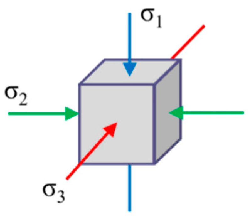
The uniaxial compression condition of concrete is too common to discuss in this section. The multi-axial stress condition can be divided into biaxial and triaxial compression conditions. In existing studies [12,13], the concrete under multi-axial compression was mainly tested using the true triaxial compressive test and the conventional triaxial compressive test. The cubic specimen in the true triaxial compressive test can be loaded under three unequal axial stresses (i.e., σ1 ≥ σ2 ≥ σ3), as shown in Figure 1. The stress conditions with unequal axial stresses can objectively reflect the actual stress conditions, such as concrete confined by a nonuniform confining effect and the section under rotational deformation. And the finite element model is mainly divided by cubic elements. Therefore, the true triaxial test results were discussed.

Figure 1.
Schematic diagram of true triaxial stress.
The biaxial compression test results of concrete are shown in Figure 2a, which reveals a parabolic relationship between the two stresses. With the increase in the middle axial stress, the maximum axial stress initially increases, followed by a decreasing trend. Based on the relationship between the two axial stresses, the different stress combinations can be analyzed to draw the following conclusions: (1) the middle stress is an important factor for the limit conditions of concrete because the maximum stress changes with the middle stress; (2) the single stress differences (i.e., σ1 − σ3, σ1 − σ2 or σ2 − σ3) cannot be key parameters because these stress differences do not reflect the parabolic relationship between the two axial stresses; (3) the maximum stress is independent of the spherical stress (σm, 3σm = σ1 + σ2 + σ3), because there may be two stress points with the same spherical stress values in Figure 2a; (4) the stress envelope curve can be represented by the maximum stress difference (σ1 − σ3) and the middle stress (σ2), based on the stress analysis in Figure 2a.
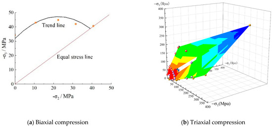
Figure 2.
Stress condition of concrete under multi-axial compression.
In order to study the mechanical properties of concrete under multi-axial compression, the test results [12,13] are summarized in 3D coordinate diagrams. If there is no axial stress order, the stress diagram can be plotted, as shown in Figure 2b. In this stress diagram, the stress points should be symmetrical about the σ1 = σ2 plane and the σ2 = σ3 plane.
Based on the 3D stress envelope, the following conclusions can be drawn: (1) The stress envelope is a “spindle-shaped surface” with the isotropic line as the central axis rather than the “open-cone-shaped surface” proposed in prior studies. The open-cone-shaped surface means that the axial stress increases continuously with the increase in hydrostatic stresses, but concrete may be crushed. The crushed concrete under high triaxial pressure will produce a spindle-shaped surface. (2) Most stress data are at lower stress levels, which just reflects the development trend of higher stress levels. (3) Hydrostatic stresses (σ1 = σ2 = σ3) strongly influence the stress conditions, which differ from the spherical stress (σm). The spherical stress is σm = (σ1 + σ2 + σ3)/3, while hydrostatic stress is the stress condition where three axial stresses are equal. There may be two stress points with equal spherical stress in the stress space. Therefore, spherical stress is an average stress, while hydrostatic stress is equal to the smallest stress. It is not appropriate to use the average stress to represent the minimum stress. (4) At the same hydrostatic stress, the relationship between the two bigger stresses is similar to the biaxial test results. (5) The hydrostatic stresses and the middle stress are key parameters to influence the stress conditions of concrete under multi-compression conditions.
2.2. Tensile Conditions
Because the tensile conditions include multi-axial tensile, tension–compression, tension–compression–compression, and tension–tension–compression, most studies have shown that lateral forces have no effect on the maximum tensile stress (σ1) of concrete. These test results [14] showed that the tensile stress of concrete is minor, which means the tensile stress loss can be ignored. Therefore, the tensile stress of concrete in any stress condition is similar to uniaxial tensile stress. But some existing studies [15,16] have shown that lateral compressive stress would reduce tensile stress. The reduced value is too small to influence the mechanical analysis. It is reasonable to take uniaxial tensile stress as a substitute for the tensile stress in the multi-axial stress condition. However, the lateral tensile stress (σ1) considerably reduces the maximum compressive stress (σ3), based on existing studies [16]. The biaxial tension–compression condition often occurs in some key members, such as the joints and the negative Poisson’s ratio structures, which would lead to critical damage.
2.3. Shear Conditions
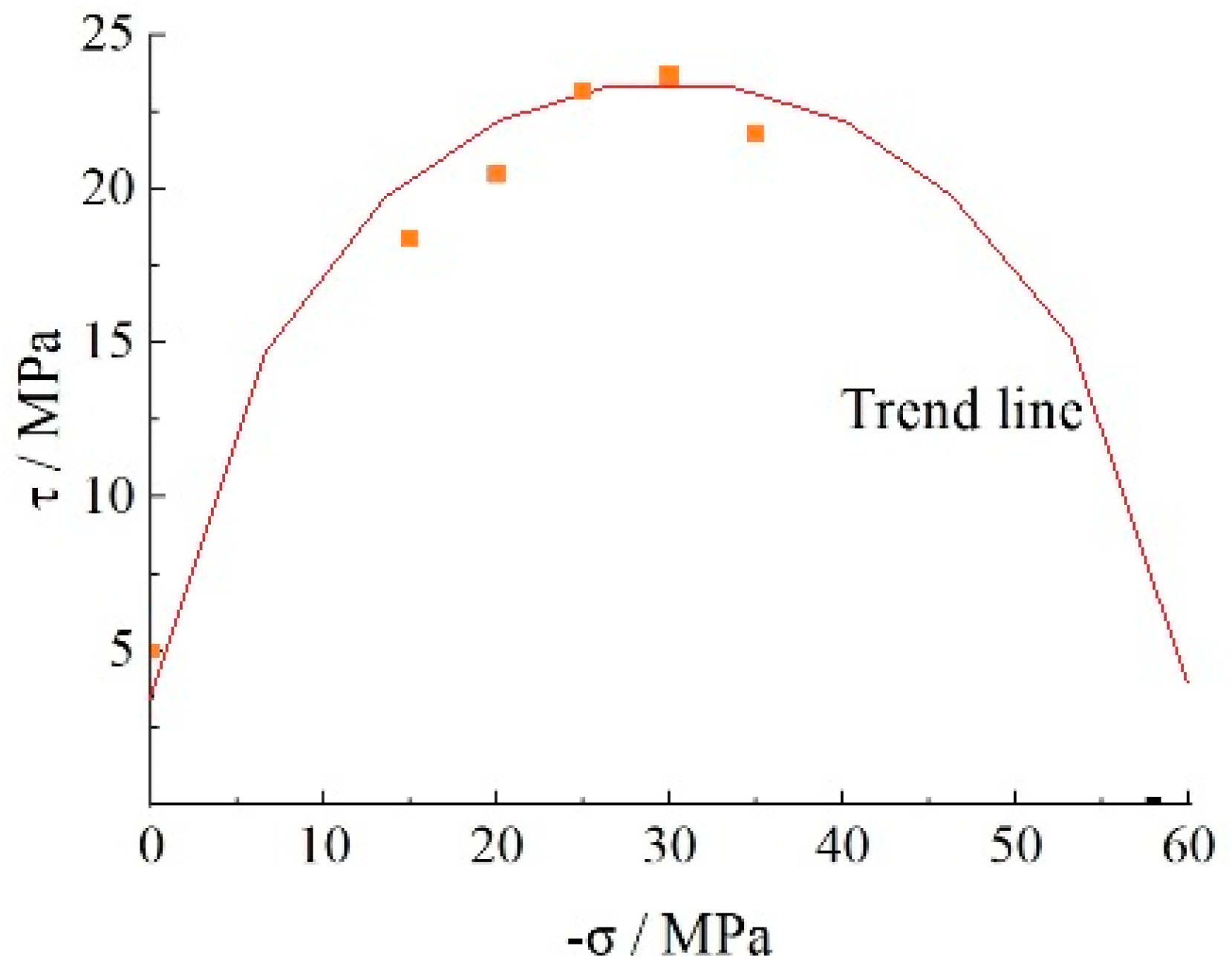
For the member under complex stress conditions (e.g., lateral shear force or torsional force), the concrete is often under the shear condition. Under the shear condition, concrete bears the combination of axial loads and shear forces. Therefore, the shear effect on the properties of the concrete is critical. Based on test results [17], the relationship between compressive stress and shear stress is drawn in Figure 3. The shear–compressive stress envelope is elliptical, which means the axial compressive stress can improve the shear stress under low-stress conditions. And the shear stress will reduce the compressive stress under high-stress conditions. It is necessary to introduce shear stresses in the failure criterion.
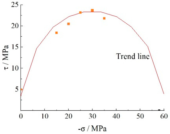
Figure 3.
Stress condition of concrete under shear–compressive condition.
In most constitutive models, the stress converted method is introduced to analyze the effect of shear stress, and to establish the failure criterion. There are some converted methods in existing failure criterion, as follows:
(1) The maximum shear stress is defined directly (see Equation (1a)). Then, the corresponding shear stresses and axial stresses are converted into the axial stresses, based on the Mohr Circles theory (see Equation (1b)).
(2) The shear and axial stresses are converted into octahedral stresses, as shown in Equation (2). The method is widely used in most failure criteria.
(3) The converted relationships between shear stresses and axial stresses are defined directly. The classical method is the double-shear unified strength theory, as shown in Equation (3).
As the analysis above shows, the converted method of the shear stresses is the key to establishing the failure criterion of concrete. The converted relationship should be proposed to reflect the mechanical properties of concrete in complex stress conditions. Therefore, it is necessary to study the mechanism of shear stress and its effect on axial stress initially. In future research, the shear stress under the lateral confining effect should be analyzed using compressive–shear tests. And the conversion mechanism of shear stress to axial stresses should be studied to propose the conversion equation.
3. Failure Criterion of Concrete under Complex Stress Conditions
The stress–strain curve of concrete can be divided into three stages: the elastic stage, the elastic–plastic stage, and the softening stage. The differences between the three stages can be reflected in loading and unloading rules, which have been discussed in existing studies [18]. The stress point between the elastic stage and elastic–plastic stage can be determined by the yield criterion. In the elastic–plastic stage, the yield surface expands with the increase in plastic strain. At the peak point, the yield surface is referred to as the failure criterion. However, the elastic stage is too short to define. It can be assumed that concrete just has the elastic–plastic stage and softening stage.
Based on above analysis, the test results of concrete under shear stress are too limited to define the converted relationship between shear stress and axial stresses. This paper only uses the axial stresses to establish the failure criterion in this section. Based on stress analysis (sees Figure 2), the key factors of the failure criterion for concrete under complex stress conditions are the middle stress (σ2), shear stress, and the hydrostatic stress.
To establish the failure criterion of concrete under multi-axial stress conditions, the first author improved the double-shear strength theory [19] to focus on the effects of shear and hydrostatic stresses. The test results show that confined concrete belongs to lower lateral stress levels (i.e., σ3: σ1 > 4). It means that shear stress is more important than hydrostatic stress. Then, the five-parameter failure criterion is proposed, as follows:
where σm is the spherical stress, σm = (σ1 + σ2 + σ3)/3; A, B1, and B2 represent the influence coefficients. It should be noted that the spherical stress is introduced to replace the hydrostatic stress [12].
In the cylindrical coordinate system, Equation (4) can be expressed as follows:
where , , , , .
To solve Equation (5), which has five unknown parameters, five stress points should be selected as the boundary conditions. The five stress points are uniaxial tensile stress (3½ α/3, 6½α/3, 0), uniaxial compressive stress (−3½/3, 6½/3, 60°), biaxial compressive stress (−2*3½ αbc/3, 6½αbc/3, 0), triaxial tensile stress (3½ α, 0, 0), and a stress point on the compressive meridian (−ξ2, ρ2, 60°). It should be noted that triaxial tensile stress is equal to the uniaxial tensile stress (i.e., σt = σttt). Based on the boundary conditions and corresponding reference [12], the parameters in Equation (5) can be expressed as follows:
The proposed model has been validated in prior research [12], and the suitable situations are where the lateral force is relatively close to and far less than the axial compressive stress. However, the model is not applicable to the following conditions: (1) there are significant differences in the three axial stresses (i.e., σ1 ≠ σ2 ≠ σ3); (2) the hydrostatic stresses are high.
Furthermore, the test results are insufficient and can only be qualitatively analyzed to identify the key factors and the influence trends. It is difficult to establish an accurate model based on the existing test results. It is necessary to propose a detailed study on concrete under multi-axial stress conditions.
4. Multi-Dimensional Constitutive Model of Concrete under Complex Stress Conditions
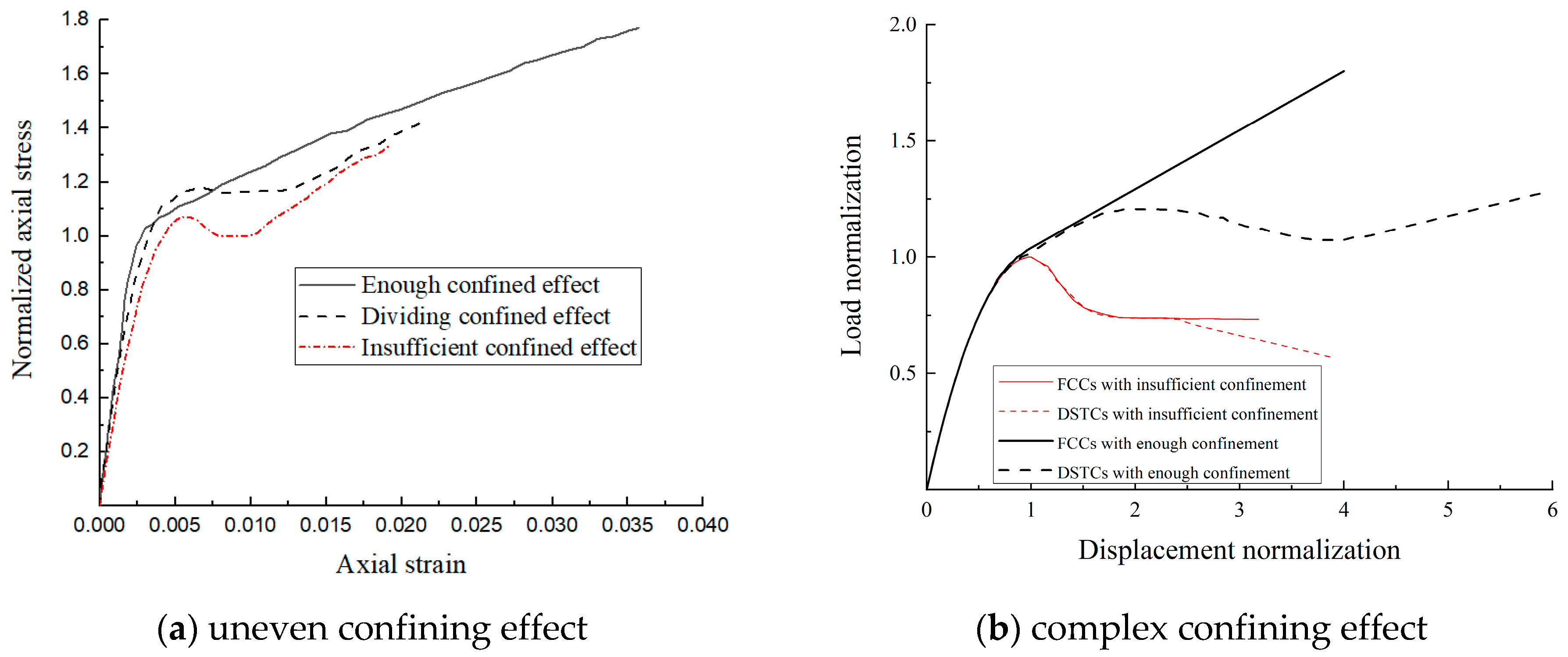
The constitutive model is the calculation method of the stress–strain curve, which is important for reflecting on the material properties. However, most existing studies only use failure criteria to compute the peak stress. And they propose the relationship curve between stress and strain. In the simple method, the relationship between the constitutive model and the failure criterion is weak, and the loading path should be set first. If the concrete is confined by uneven lateral pressure or under other complex stress conditions, the stress–strain curve will be difficult to predict (see Figure 4) [18]. Therefore, these simple constitutive models are not suitable for concrete under complex stress conditions. To solve the above problems, it is necessary to present a theoretical analysis of the failure criterion and identify the key parameters of the stress–strain curve.
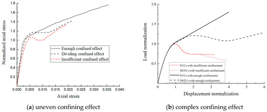
Figure 4.
The stress–strain curve of concrete confined by complex pressure.
Based on the existing studies [20,21], the stress–strain curve can be directly divided into the elastic–plastic stage and the softening stage. Therefore, it is necessary to establish relationships between the stress–strain characteristics and the failure criteria. Then, the multi-dimensional constitutive model of concrete can be established by iterative processes based on the plastic deformation, the hardening trend, and the softening trend.
4.1. Elastic–Plastic Stage
4.1.1. Multi-Dimensional Elastic–Plastic Constitutive Model
In each iteration step, the strain increment (dε) includes the elastic strain (dεe) and the plastic strain (dεp), i.e., dε = dεe + dεp. Then, the stress increment can be expressed as follows:
where [De] is the elastic matrix, as follows:
where K is the Bulk modulus, G is the shear modulus, ν is the Poisson’s ratio.
The key parameters should be derived again to form the new derivation process for computing software. Based on the generalized plasticity theory, the plastic strain increment is:
where dλ is the plastic multiplier, A is the plastic modulus, nl is the unit vector perpendicular to the yield surface (f).
It should be noted that when the stress point is on the yield surface, the direction of strain increment (nl) is determined by the yield surface. If the stress point is at the yield surface, the direction of strain increment (n) should be determined by the plastic energy surface (g). If the associated flow rule is adopted, the yield surface should be equal to the plastic potential energy surface, as follows:
By combining Equations (6)–(9), as follows:
Then, by combining Equations (6), (8), and (9), as follows:
4.1.2. Initial Plastic Modulus
In the elastic–plastic stage, the plastic modulus on the yield surface can be obtained by the coordination equation of the boundary interface, as follows:
where Hn is the hardening parameter, which can be the corresponding spherical stress when the generalized shear stress is zero (i.e., J2 = 0).
By combining Equations (8) and (12), as follows:
Based on the critical state model, the volumetric strain variation equation:
where k is the material parameter, which relates to material characteristics (e.g., Poisson’s ratio and plasticity properties).
By combining Equations (13) and (14), the plastic modulus is:
4.2. Softening Stage
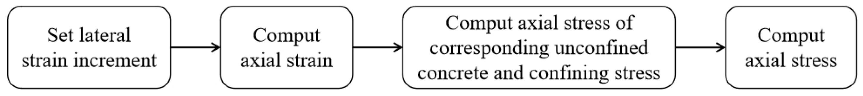
Based on study [13], the significant damage leads to the softening process of concrete. Therefore, the softening process is the degradation process of mechanical properties, which means the failure surface shrinks constantly. The study [13] used the energy method to predict the softening properties of confined concrete. The study results show that the strain dissipation energy of unconfined concrete and three types of actively confined concrete are the same. Therefore, the dissipation energy can be used as the foundation for predicting the softening curve in further research. It means that the strain calculation model can be established by adjusting the constitutive model of unconfined concrete. The calculation iteration process is shown in Figure 5, which has been published in the study [13]. Then, the compiled program can be applied in this paper.

Figure 5.
Calculation iteration process of the softening curves.
The above process can provide relatively accurate prediction results for conventional confined concrete. However, the study is presented by experimental analysis. It cannot predict the stress–strain curve of concrete in complex stress conditions, as shown in Figure 4b. It is not possible to provide a more scientific explanation for the softening stage, and connect it with the failure criterion because of lack of test data and theoretical analysis. The solutions will be discussed in the following section.
4.3. Cycle Loading
4.3.1. Loading–Unloading Path
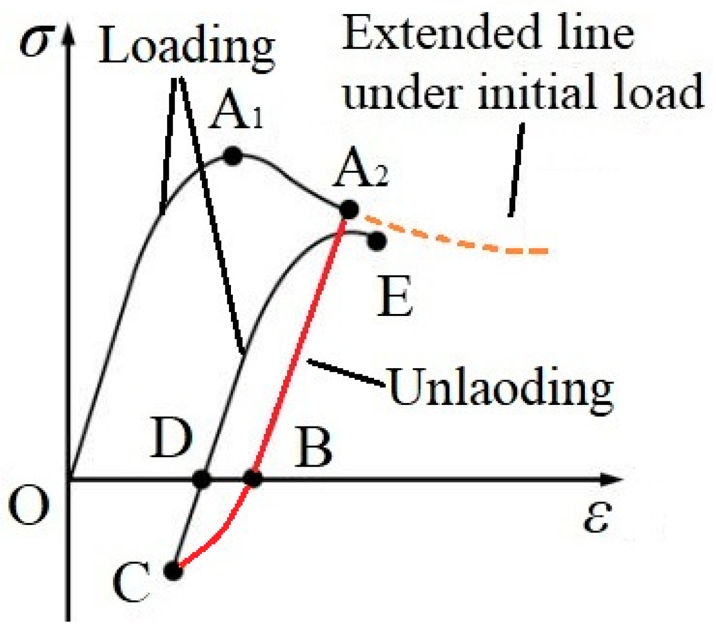
In this section, the two-stage curve is an example to describe the mechanical properties of concrete in the cyclic loading path, as shown in Figure 6. The cyclic stress–strain curve includes the following stages. (1) initial loading stage (i.e., OA path), which includes the elastic–plastic rise stage (i.e., OA1 path) and the softening stage (i.e., A1A2 path); (2) unloading stage (i.e., AB path), which shows an elastic trend, which means the plastic displacement would not change until unloading completion; (3) reloading stage (i.e., BC path), which shows an elastic–plastic trend; (4) re-unloading stage (i.e., CD path), which shows an elastic trend; (5) reloading stage (i.e., DE path), which shows an elastic–plastic trend. Based on the above rules, the loading–unloading path is set. And the plastic modulus in the process will be discussed in the following section, which outlines the mapping rule.

Figure 6.
Stress-strain curve of concrete in the axial cyclic loading.
Based on the above analysis, there are two obvious states, namely, the loading state and the unloading state. There are two judging conditions. When σ*dε < 0, the stress point is in the unloading state, and the stress–strain curve shows an elastic trend. When σ*dε ≧ 0, the stress point is in the loading state, and the stress–strain curve shows an elastic–plastic trend. The elastic–plastic curve should be calculated by Equation (11), which uses the plastic modulus to reflect the plastic property. It should be noted that concrete experiences continuous damage with increasing plastic deformation. The concrete damage leads to the following stress characteristics: (1) the peak stress (E) of the reloading curve is lower than the unloading stress (A2); (2) the unloading stiffness is lower than the elastic modulus, which will decrease as the damage increases.
4.3.2. Plastic Modulus and Mapping Rule
As discussed in Section 4.1.1, the plastic modulus is defined to compute the stress and strain increments. If the stress point is within the yield surface, the plastic potential energy surface should be determined by the mapping rule. The mapping rule of the incremental boundary surface can refer to the existing radial mapping rule [22]. And the strain increment direction is known because the plastic potential energy surface is similar to the yield surface.
In this section, the yield surface in the p-q stress space is an example to discuss the mapping rule of the boundary surface, as shown in Figure 7. The mapping point (p0, q0) on the yield surface is the intersection point between the yield surface and the mapping line. The mapping line passes the origin point and the stress point (pn, qn). Therefore, there is a unique mapping point on the yield surface corresponding to the stress point. And δ0 and δ are distance from the origin point and the stress point to the mapping point, respectively. Then, the corresponding plastic modulus on the plastic potential energy surface is established by the interpolation method, based on the stress distance.
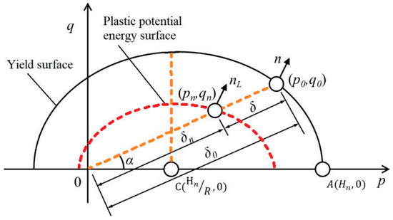
Figure 7.
Mapping rule in p-q stress space.
The plastic modulus can be computed as follows:
where m is the reduction parameter caused by the plastic strain.
4.4. Calculation Steps and Programs
In the proposed derivation process, some initial parameters should be set first, including the elastic matrix, the calculation method of the yield function and plastic modulus, the strain increment (dε), and targeted strain path. Then, plastic strain increment should be calculated by the current stress condition and the corresponding calculation method. Finally, the stress increment should be calculated by the plastic strain, and the new stress condition is updated to begin the new cycle steps. The detailed process of the proposed constitutive model can be established by the following steps:
- (1)
- Determine the stress condition. If it is not a cyclic process, the step should calculate the hardening parameter (Hn) using the yield function (f) and the current stress condition. If it is a cyclic process, the step should compute the mapping point (p0, q0).
- (2)
- Compute the plastic modulus (A). The value can be computed by Equations (15)–(17).
- (3)
- Compute the stress increment and the plastic stain by Equation (11). Then, the process can obtain the stress point in the next step.
- (4)
- Judge whether the stress exceeds the peak stress. If it does, the step should use the iteration process of the softening curve to recalculate the stress point.
- (5)
- Update the new yield surface equation and new stress point. It should be noted that the hardening parameter is not updated in the cyclic process.
The above steps can be expressed in the process shown in Figure 8. In the calculation process, some key parameters should be set or calculated, which are clarified as follows: In the first step, the yield function should be selected. In this paper, the yield function was expressed in Equation (4). And the special stress point (p = 0) is introduced into Equation (4) to compute the hardening parameter (Hn). Then, the current stress point (p, q) is used to compute the mapping point (p0, q0). In the second step, the plastic modulus (A) is computed by the envelope plastic modulus (And) and Equations (15)–(17). And the equation of envelope plastic modulus (And) is And = a*exp(−b*ε) + c*exp(−d*ε). In the third step, the plastic strain and stress are computed by the yield function, the elastic matrix, and the strain increment in Equation (11). In the fourth step, the computed stress should be assessed. If the computed stress is over peak stress, the stress should be recalculated by the energy method, which has been studied by the first author. In the fifth step, the stress point and yield function are summarized and then updated in the subsequent cycle steps. It should be noted that all parameters in the above steps should be defined by material test and analysis, such as the elastic matrix, the yield function, and the softening function. This section provides an approach for linking material properties with the mechanical performance of composite structures. Therefore, the corresponding parameters should be changed for different materials.
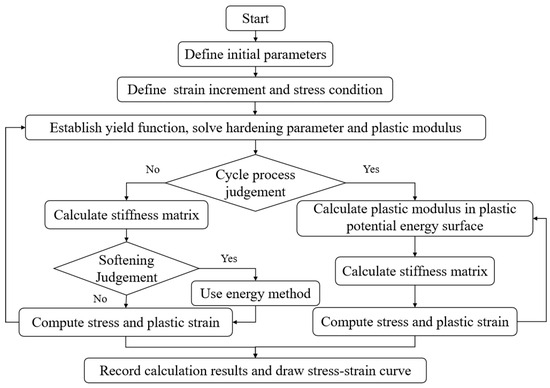
Figure 8.
Solution program of the constitutive model of concrete.
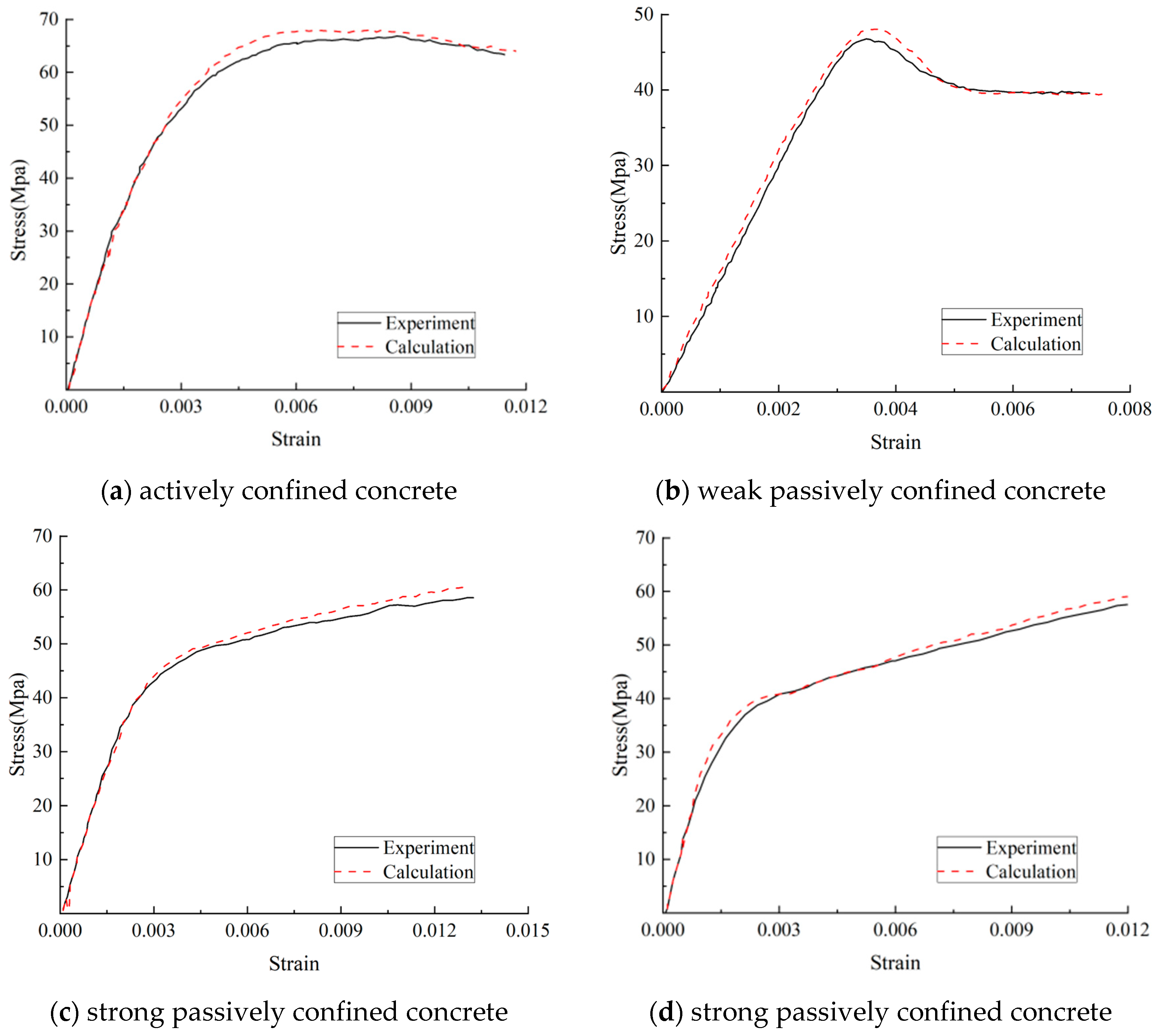
4.5. Model Verification
This section verifies the proposed model by calculation results and test results. The test results [12,18] belong to the confined concrete under uniaxial loading, including actively and passively confined concrete. The curve comparisons are shown in Figure 9. The verification results show that the proposed model can provide accurate prediction results and have wide applicability. However, the proposed model has many limitations, and can only apply to ordinary concrete. The accurate mode should be based on an extensive reasonable database. Afterward, future research should analyze the mechanical mechanism and identify the key influence factors. In this model, the elastic model of confined concrete is 30 GPa. The yield function is shown in Equation (5b), where b0 = 15, b1 = 146, b2 = 873. In the equation of And, a = 2.2 × 10⁸, b = 1.96, c = 1.05 × 10³, d = 1.11. It should be noted that the parameters are valid compared to previous studies, but the parameters should be reset by new materials.
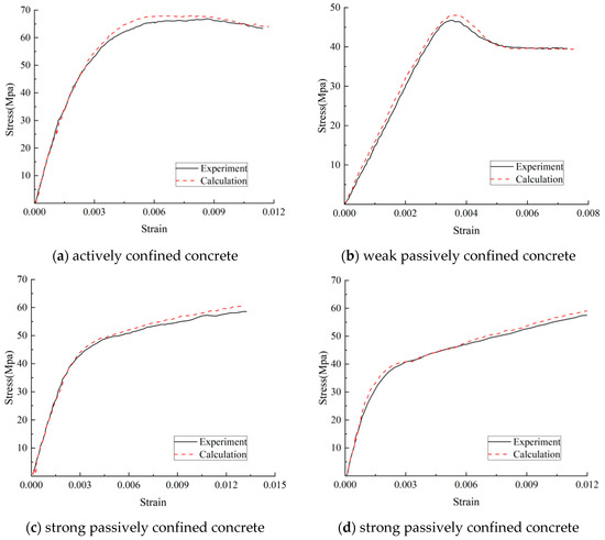
Figure 9.
The model verification of confined concrete.
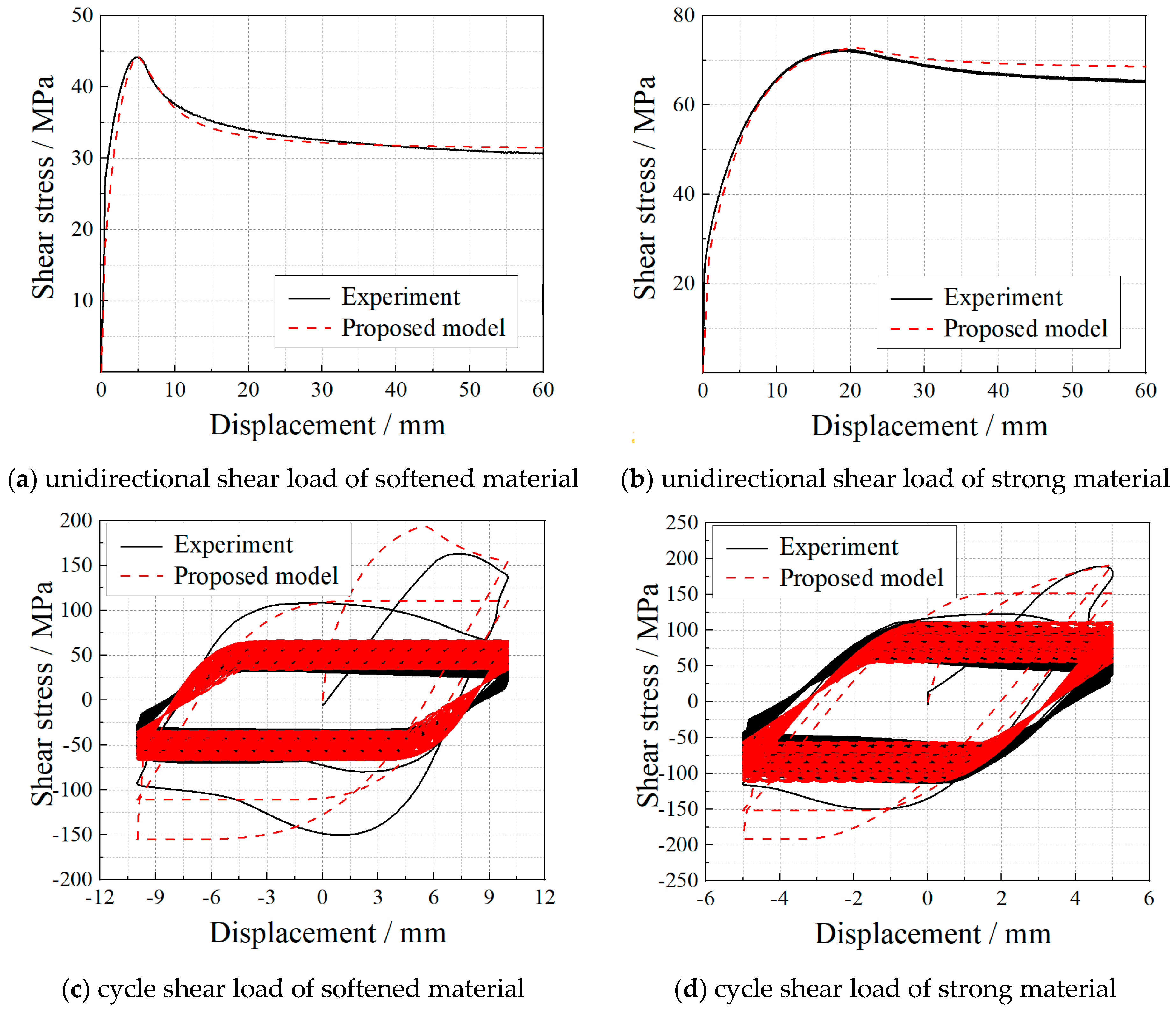
Since there are few cyclic curves for concrete, this paper uses the cyclic shear test results [23] of soil to verify the proposed constitutive model. The verification curves include the single shear curve and the cyclic shear curve, as shown in Figure 10. It can be seen that the peak stress of each cycle curve decreases with the increase in the cycle number. And the stress reduction value also continuously decreases till constant. The verification results in Figure 10 show that the proposed model can provide accurate prediction results for cyclic shear tests. In this model, the elastic model of confined concrete is 7.3 GPa. The yield function is the Cambridge model, where R = 3. In the equation of And, a = 7.3 × 10¹⁰, b = 6.6, c = 3.38 × 10⁴, d = 1.3. It should be noted that the parameters are valid compared to previous studies, but the parameters should be reset by new materials.

Figure 10.
The model verification of soil under shear loading.
5. Conclusions
For a complex structural system, the concrete in key members would be under complex stress conditions. It is necessary to clear the properties of the core concrete for accurate mechanical analysis. Therefore, this paper studied the mechanical mechanism of concrete under complex stress conditions to propose the failure criterion, including multi-axial compression, multi-axial tension–compression, and shear–compression conditions. Then, the calculation methods of the constitutive model were derived by stiffness matrix, plastic modulus, stress, and strain increment. Finally, the failure criterion was applied to each analysis step to establish the constitutive model based on the proposed iterative process. As mentioned above, the proposed model has a theoretical derivation process and can predict the mechanical properties of concrete under complex stress conditions by basic material parameters. Based on the above study, the following conclusions can be drawn:
- (1)
- The stress envelope diagram of concrete under multi-axial stress conditions shows the “spindle” shape with the isoclinic line as the central axis, which passes through the axis origin. This is because the concrete may be crushed under high triaxial pressure, which will produce a spindle-shaped surface.
- (2)
- The hydrostatic stresses (σ1 = σ2 = σ3) have an obvious effect on the limit condition of concrete under multi-axial compression, which differs from the spherical stress (σm) used in most existing studies because there may be two equal spherical stress points in the stress space. Therefore, spherical stress is an average stress, while hydrostatic stress is equal to the smallest axial stress.
- (3)
- The middle stress, the shear stress, and the hydrostatic stress can establish the failure criterion model. However, the effect of shear stress under confining pressure is hard to express by characteristic stresses, which should be clarified in future studies.
- (4)
- In the iterative calculation process of the proposed constitutive model, the hardening parameter is the key to reflecting the yield surface. And the hardening parameter can be reflected by the plastic modulus, based on corresponding formula derivation.
- (5)
- The plastic modulus is the key to reflecting plastic behavior, including the plastic development trend and the cycle of mechanical behavior. Therefore, the calculation method of plastic modulus is the key to establishing the constitutive model. And the true triaxial test results are the most important parameters that should be focused on in the future.
In this paper, the proposed model can predict the mechanical properties of concrete under complex stress conditions. However, the study results are far from meeting the analysis requirements, for the following reasons: First, there is a lack of experimental results on concrete under high multi-compression conditions. Especially, the test results of concrete under 100 MPa-confining pressure are too few to allow for a detailed analysis of the yield surface of concrete under complex stress conditions. Second, there are few studies that focus on the mechanical properties of concrete under multi-axial tension–compression conditions, which is common in practical engineering. Third, the theoretical foundation is not enough to clarify the converted method for the elliptical relationship between axial stresses and shear stress. It is necessary to supplement relevant experimental studies and theoretical analysis in the future, especially for the mechanical mechanism and mathematical expression of concrete under complex stress conditions.
Author Contributions
Conceptualization, C.R., Z.D. and J.T.; methodology, C.R. and Z.D.; validation, C.R. and J.T.; formal analysis, C.R. and Z.D.; investigation, J.T.; data curation, Z.D.; writing—original draft preparation, C.R.; writing—review and editing, C.R., Z.D. and J.T.; visualization, C.R. and Z.D.; supervision, C.R.; funding acquisition, C.R. and J.T. All authors have read and agreed to the published version of the manuscript.
Funding
This work is supported by the National Natural Science Foundation of China [grant number 52108171] and the China–Pakistan Belt and Road Joint Laboratory on Smart Disaster Prevention of Major Infrastructures [grant number 2022CPBRJL-11].
Data Availability Statement
The raw data supporting the conclusions of this article will be made available by the authors on request.
Acknowledgments
The authors gratefully acknowledge the Key Laboratory at Xi’an University of Architecture and Technology for the experiments. This work is supported by the National Program on Key R&D Project of China (2022YFE0210500) and the Open Research Project of the China–Pakistan Belt and Road Joint Laboratory on Smart Disaster Prevention of Major Infrastructures.
Conflicts of Interest
The first and second author are employed by the Xi’an University of Architecture and Technology. The third author is employed by the Quakesafe Technologies Co., Ltd.
References
- Cui, J.; Hao, H.; Shi, Y.; Li, X.; Du, K. Experimental study of concrete damage under high hydrostatic pressure. Cem. Concr. Res. 2017, 100, 140–152. [Google Scholar] [CrossRef]
- Khusru, S.; Thambiratnam, D.P.; Elchalakani, M.; Fawzia, S. Behaviour of slender hybrid tubberised concrete double skin tubular columns under eccentric loading. Buildings 2024, 14, 57. [Google Scholar] [CrossRef]
- Khusru, S.; Thambiratnam, D.P.; Elchalakani, M.; Fawzia, S. Load-displacement behaviour and a parametric study of hybrid rubberised concrete double-skin tubular columns. Buildings 2023, 13, 3131. [Google Scholar] [CrossRef]
- Tayeh, B.A.; Akeed, M.H.; Qaidi, S.; Bakar, B.H.A. Behavior of eccentrically loaded hybrid fiber-reinforced high strength concrete columns exposed to elevated temperature. Case Stud. Constr. Mater. 2022, 17, e01495. [Google Scholar] [CrossRef]
- Mukhtar, F.; Deifalla, A. Shear strength of FRP reinforced deep concrete beams without stirrups: Test database and a critical shear crack-based model. Compos. Struct. 2023, 307, 116636. [Google Scholar] [CrossRef]
- Ozbakkaloglu, T.; Lim, J.C. Axial compressive behavior of FRP-confined concrete: Experimental test database and a new design-oriented model. Compos. Part B Eng. 2013, 55, 607–634. [Google Scholar] [CrossRef]
- Zhang, X.; Chen, P.; Wang, H.; Xu, C.; Wang, H.; Zhang, L. Constitutive model of FRP tube-confined alkali-activated slag lightweight aggregate concrete columns under axial compression. Buildings 2023, 13, 2284. [Google Scholar] [CrossRef]
- Wang, L.; Huang, X.; Xu, F. Stress-Strain model of high-strength concrete confined by lateral ties under axial compression. Buildings 2023, 13, 870. [Google Scholar] [CrossRef]
- Amin, M.; Agwa, I.S.; Mashaan, N.; Shaker, M.; Abd-Elrahman, M.H. Investigation of the physical mechanical properties and durability of sustainable ultra-high performance concrete with recycled waste glass. Sustainability 2023, 15, 3085. [Google Scholar] [CrossRef]
- Pressmair, N.; Brosch, F.; Hammerl, M.; Kromoser, B. Non-linear material modelling strategy for conventional and high-performance concrete assisted by testing. Cem. Concr. Res. 2022, 161, 106933. [Google Scholar] [CrossRef]
- Liang, M.; Chang, Z.; Wan, Z.; Gan, Y.; Schlangen, E.; Šavija, B. Interpretable Ensemble-Machine-Learning Models for Predicting Creep Behavior of Concrete. Cem. Concr. Compos. 2022, 125, 104295. [Google Scholar] [CrossRef]
- Rong, C.; Shi, Q.; Zhang, T.; Zhao, H. New Failure Criterion Models for Concrete under Multiaxial Stress in Compression. Constr. Build. Mater. 2018, 161, 432–441. [Google Scholar] [CrossRef]
- Rong, C.; Shi, Q. Analysis Constitutive Models for Actively and Passively Confined Concrete. Compos. Struct. 2021, 256, 113009. [Google Scholar] [CrossRef]
- Yang, H.; Fang, J.; Jiang, J.; Li, M.; Mei, J. Compressive Stress–Strain Curve of Recycled Concrete under Repeated Loading. Constr. Build. Mater. 2023, 387, 131598. [Google Scholar] [CrossRef]
- Gao, X.; Wang, W. Component Model and Design Method for Tensile Behavior of Slip-Critical Blind Bolts Anchored in Concrete-Filled Steel Tubular Sections. Thin-Walled Struct. 2023, 186, 110701. [Google Scholar] [CrossRef]
- Kim, H.-Y.; Yang, K.-H.; Lee, H.-J. Tensile Stress–Strain Relationship of Fiber-Reinforced Concrete with Different Densities. Constr. Build. Mater. 2023, 385, 131526. [Google Scholar] [CrossRef]
- Luo, X. Study on Dynamic Behavior and Damage Characteristics of Concrete under Compression and Shear State; Three Gorges University: Yichang, China, 2017. [Google Scholar]
- Rong, C.; Shi, Q.; Zhao, H. Behaviour of FRP Composite Columns: Review and Analysis of the Section Forms. Adv. Concr. Constr. 2020, 9, 125–137. [Google Scholar] [CrossRef]
- Yu, M.-H. Unified Strength Theory and Its Applications; Springer: Singapore, 2018; ISBN 978-981-10-6246-9. [Google Scholar]
- Li, Y.; Guo, H.; Zhou, H.; Li, Y.; Chen, J. Damage Characteristics and Constitutive Model of Concrete under Uniaxial Compression after Freeze-Thaw Damage. Constr. Build. Mater. 2022, 345, 128171. [Google Scholar] [CrossRef]
- Liao, J.; Zeng, J.-J.; Dai, H.-S.; Chen, W.-J.; Zhou, J.-K. A Constitutive Model of Expansive Concrete and Steel Fiber-Reinforced Expansive Concrete under Tri-Axial Compression. Compos. Struct. 2023, 320, 117212. [Google Scholar] [CrossRef]
- Zienkiewicz, O.C.; Leung, K.H.; Pastor, M. Simple Model for Transient Soil Loading in Earthquake Analysis. I. Basic Model and Its Application. Int. J. Numer. Anal. Methods Geomech. 1985, 9, 453–476. [Google Scholar] [CrossRef]
- Feng, S.-J.; Shi, J.-L.; Shen, Y.; Chen, H.-X.; Chang, J.-Y. Dynamic Shear Behavior of GMB/CCL Interface under Cyclic Loading. Geotext. Geomembr. 2021, 49, 657–668. [Google Scholar] [CrossRef]


Disclaimer/Publisher’s Note: The statements, opinions and data contained in all publications are solely those of the individual author(s) and contributor(s) and not of MDPI and/or the editor(s). MDPI and/or the editor(s) disclaim responsibility for any injury to people or property resulting from any ideas, methods, instructions or products referred to in the content. |
© 2024 by the authors. Licensee MDPI, Basel, Switzerland. This article is an open access article distributed under the terms and conditions of the Creative Commons Attribution (CC BY) license (https://creativecommons.org/licenses/by/4.0/).