Effect of Soil–Bridge Interactions on Seismic Response of a Cross-Fault Bridge: A Shaking Table Test Study

Abstract

A shaking table test of a 1/60 scale cross-fault bridge model considering the effects of soil–bridge interactions was designed and implemented, in which the bridge model was placed in two individual soil boxes to simulate the bridge across a strike-slip fault. Three seismic ground motion time-histories with permanent displacements were selected as input excitations to investigate the influence of seismic ground motions with different frequency characteristics on the seismic response of the testing soil–bridge model. The one-side input method was used to simulate the seismic response of bridges across faults. The seismic responses of the soil and bridge in terms of acceleration, strain, and displacement were analyzed. The test results show that the one-side input method can simulate the seismic response of the main girder displacements well and the displacements and strains of piers and piles of the bridge structure spanning a fault. The strain responses at near-fault pile foundations are much larger than those farther away from the fault. Compared with other bridges, the cross-fault bridge is more prone to torsional and displacement responses during earthquakes. Surface fault rupture can lead to permanent inclination of the bridge piers, which should be paid more attention to in the practical engineering design of the bridges. Soil–bridge interactions can suppress the amplification effect of soil on ground motions. The test results can provide a reference for future research and the design of cross-fault bridges.

1. Introduction

At present, research on the seismic resistance of cross-fault bridges is still in an early stage [1]. Seismic design and construction regulations mostly follow the principle of avoidance when dealing with active fault zones [2,3,4,5]. However, with the rapid development of highway and railway bridges, this principle has become difficult to meet in practice. It is estimated that in the earthquake-prone California, more than 5% of bridges may cross or be very close to fault rupture [6,7]. China has the most complex active tectonic system with the largest number of known active faults [8]. In recent years, transportation infrastructure has developed rapidly in China, especially in the southwestern mountainous region and southeastern coastal area, resulting in a significant increase in the number and density of newly built bridges. There are many large-scale active fault zones in China, and some are up to thousands of kilometers in length, such as the Tanlu fault zone in the east and the Kunlun and Longmenshan fault zones in the southwest. Based on a consideration of various factors, including road planning, engineering costs, construction time, and regional economic development, bridge construction on the sites near or across active faults in China has become an unavoidable problem [5]. These bridge projects are often the transportation hubs or even the lifeline engineering of a certain region. Therefore, seismic performance of cross-fault bridges has become an urgent topic in seismic engineering research.

Cross-fault bridges refer to bridge structures that span an active fault, with piers or abutments on both sides of the fault. During an earthquake, the piers and abutments on both sides of fault will withstand a relative displacement due to the fault dislocation [1,9,10,11]. The moments at the bottom and transverse bearing displacements at the top of piers immediately adjacent to the fault are much larger than those at other locations [12,13,14]. The relative displacement and permanent displacement on both sides of a fault are the main characteristics of ground motion across both sides of the fault during an earthquake, which are also the main factors causing damage to bridge structures [15,16,17,18,19,20,21,22]. Previous studies have conducted few tests that simultaneously consider fault dislocations and ground motions [18]. Some tests were conducted using a shaking table array with two sub-tables to simulate the relative motion and permanent displacement on both sides of the fault, in which equally large reverse ground motion time-histories contain permanent displacement into both shaking tables [9,23]. Although these tests can effectively simulate the seismic response of cross-fault bridge structures, there are still technical challenges in pursuing more convenient and high-quality cross-fault seismic test reproduction. The main problems include the following: (1) due to test conditions, it is difficult for general laboratories to carry out shaking table tests of bridge structures across faults with multiple sub-tables of such large shake tables; (2) in shaking table tests, it is difficult for conventional input methods to reproduce the permanent displacement of ground motion due to the influence of the protection mechanism of the shaking table itself (its own frequency range). It is worth exploring how to achieve the test reproduction of permanent ground displacement in cross-fault seismic motion and the input control method of the shaking table; (3) there is an issue of the reproduction accuracy of multi-dimensional and multi-point input cross-fault ground motions in the shaking table array system, especially the multi index reproduction accuracy of high-frequency acceleration and low-frequency displacement; (4) significant displacement demand may be generated due to fault displacement, which may lead to direct damage to the test model. Therefore, the traditional step-by-step loading system may not be applicable [18]. (5) When designing shaking table tests, the participation of soil makes the design of similar soil–structure systems extremely complex. Previous studies have shown that the participation of soil has an important influence on the seismic response of bridges and is an unavoidable issue [24,25]. Meanwhile, the effect of the difference in large deformations of the permanent ground displacement on both sides of the earthquake fault on the seismic performance of bridge structures needs to be further explored [5].

1.1. Design of Shaking Table Test

In order to study the effect of permanent displacement caused by fault dislocations on the seismic response of cross-fault bridges, this paper conducted shaking table tests using a typical 1/60 scale model of a continuous box girder bridge. This study analyzes the dynamic response of a soil-bridge system under seismic loads based on test data and visual observations. Based on previous research and its shortcomings, the following attempts were made in the shaking table tests:

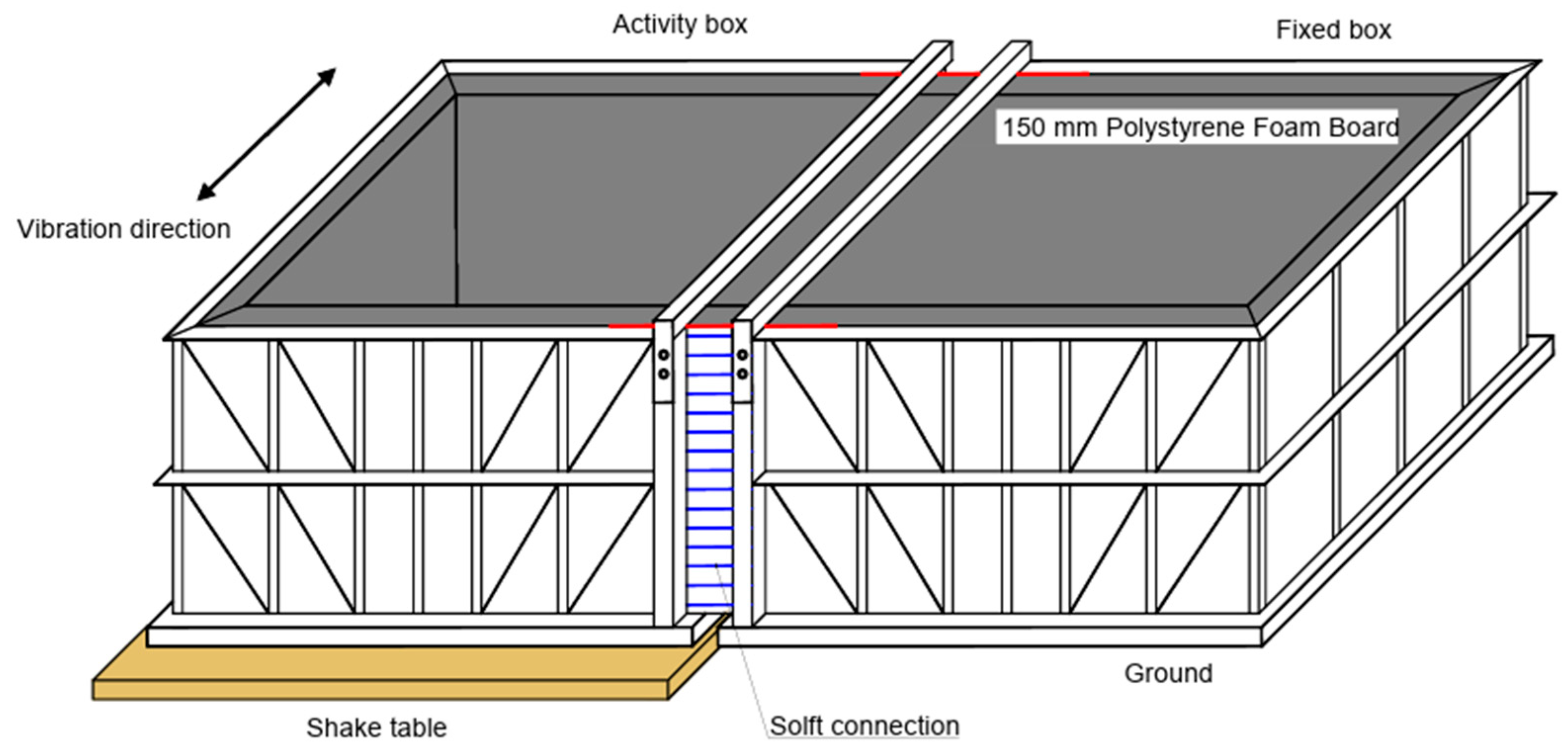
• This study attempts to simulate different ground motions on both sides of the fault with only one shaking table. The soil box is divided into two parts; one half is resting on the shaking table and the other half is fixed on the ground, connected with a steel strand in the middle. The displacement difference on both sides of the fault is used as the input of the shaking table to simulate the impact of the relative displacement and permanent displacement of the fault on the seismic response of the bridge structure, i.e., one-side input method.
• During the tests, displacement control shaking table input is adopted to ensure that the relative permanent displacement on both sides of the fault can be reproduced.
• In the tests, polymethyl methacrylate is used as the model material to improve the design stiffness of the test model.
• This test refers to the experimental similarity design method proposed by Xu, using the predominant period, time, and displacement of the site as the basic similarity conditions to maintain the main characteristics of the original site in the model soil, which can ensure partial similarity between the soil–structure system model and the prototype [26].

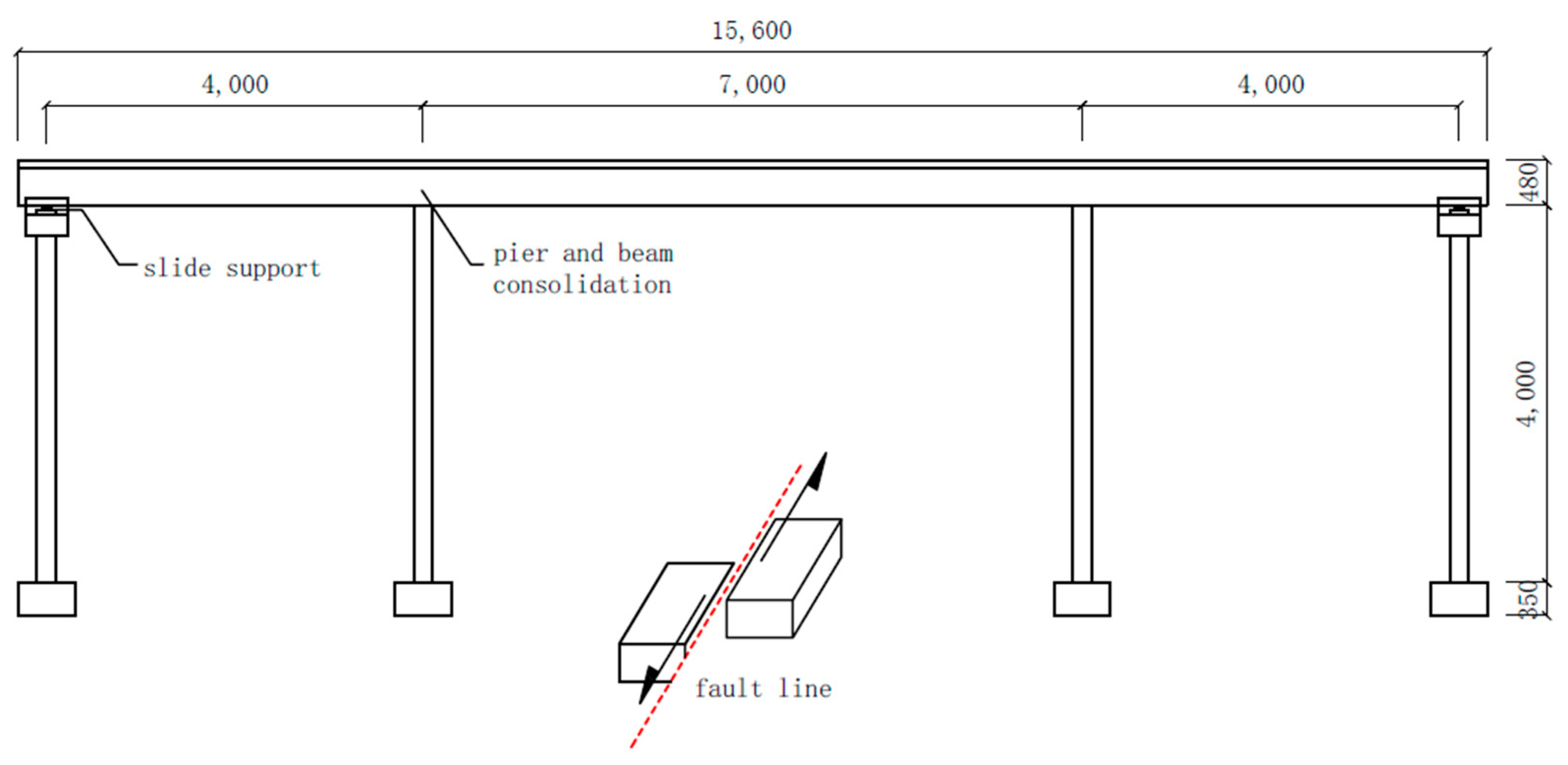
1.2. Prototype Bridge

The prototype for this test is the Haiwen Bridge in Hainan Province, China. The main part of the bridge is composed of three-span continuous concrete single-box girders, with a total length of 42 + 60 + 42 m. The beam is 35 m wide and 6 m high, and the box girder is a single-box single structure of C40 concrete. The substructure uses vase-shaped piers for both the middle and side piers, with beam-pier connection used for the middle pier to strengthen the lateral stability of the bridge, and double-plate rubber bearings are installed at the top of side piers. All foundations are 2 × 2 pile groups with a diameter of 4.5 m.

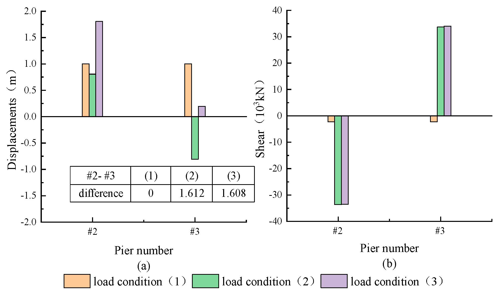
1.3. Numerical Confirmation of Single-Side Input Motion

Differences in ground motions with permanent displacements on the two sides of the fault caused by fault rupture are the main factors affecting the internal forces and deformations of the cross-fault bridge during earthquakes. Due to the limitations of the test condition, only one shake table is available, so it is impossible to simultaneously load seismic motions on both sides of the fault. Therefore, one-side input is used to simulate the different ground motions on the two sides of the fault and their effects on the cross-fault bridge structure.

The feasibility of the single-side input approach was numerically confirmed using the finite element software Csi-Bridge (2020). For this purpose, a model of a three-span continuous box girder bridge with a total length of 40 + 70 + 40 m and piers heights of 40 m is established, as shown in Figure 1. The piers are 1 m in thickness and 6 m in width. The main girder has a single-chamber box section with a width of 6 m and a height of 4.8 m. The plate is 6 m wide, with the top plate being 0.28 m thick and the bottom plate 0.25 m thick. The web plate thickness is 0.4 m. In the test, we focus on structural displacement and the internal force response [7,20,21].

To assess the variations in structural responses induced by different displacement loading methods, three loading scenarios were employed in the transverse direction of the bridge. For loading scenario 1, identical displacement time-histories with a permanent displacement were applied at the base of each pier to simulate the seismic effects on a bridge near a fault. For loading scenario 2, the same displacement time-histories from loading scenario 1 were applied at the bottoms of piers #1 and #2. Conversely, these displacement time-histories were inverted (multiplied by −1) for piers #3 and #4 to simulate the seismic response of the bridge crossing the fault. For the loading scenario 3, the displacement time-histories of loading scenario 1 were doubled in amplitude and applied to the bases of piers #1 and #2 to simulate the effects of different motions on a cross-fault bridge. The displacement inputs for the three scenarios are shown in Figure 2, and the resulting displacements at the top and shear forces at the bottom of piers #2 and #3 are compared in Figure 3. For loading scenario 2 and 3, the relative displacement of pier tops adjacent to the fault (pier #2 and #3) is approximately the same and greater than those in loading scenario 1. And these identical relative displacements of loading scenario 2 and 3 lead to closely matching shear forces at piers #2 and #3, as shown in Figure 3b. Consequently, it is inferred that the structural responses, such as the shear force, bending moment, torsion, etc., are approximately the same for loading scenario 2 and 3. This analysis suggests that the third loading scenario effectively models the seismic impacts of varying ground movements on either side of a fault on the seismic performance of cross-fault bridges.

1.4. Similarity Analysis

For the soil–bridge interaction system, the presence of soil makes the similarity relations and scaling factors extremely complex. It is very difficult to keep the similarity ratios of the elastic modulus and density of soil consistent with those of the bridge structure. In the tests, the displacement time-history was used as input, and the site’s dominant period has a significant influence on the seismic response of the structure. Therefore, the bridge length, dominant period, and periodicity were selected as the basic physical quantities to design the similarity ratio of soil, which retains the main characteristics of the original site to ensure sufficient similarity between the soil–bridge system model and its prototype [26,27,28]. The similarity relationship of the test soil–bridge model is shown in

Table 1. Similarities.

Physical Quantities	Similarities	Bridge	Soil	Physical Quantities	Bridge	Structure	Soil
Young’s modulus similarity $E$	$S_E$	1/10	1/8	Periodicity T	$S_T=\sqrt{S_L/S_a}$	0.053	0.047
Equivalent density $\rho$	$S_{\rho }$	1	1	Frequency f	$S_f=\frac{1}{S_T}$	18.97	21.27
Length $l$	$S_l$	1/60	1/60	Acceleration a	$S_a=\frac{S_E}{S_L{S}_{\rho }}$	6	7.5

. For ease of differentiation, $S$ denotes the bridge structural similarity ratio and $S^s$ denotes the soil similarity ratio.

(1)

Bridge structural model similarity ratio design

Considering soil–pile–structure interaction, the dynamic response of the structure is driven by the soil-to-pile movement; therefore, the structural acceleration similarity ratio should be consistent with the soil. For the bridge structure model, the commonly used materials are, for example, concrete, cement mortar, fine stone concrete, and polymethyl methacrylate. According to the size of the shaking table and bearing capacity of the laboratory, the size similarity ratio of the bridge structural model $S_L$ is designed as 1/60. This test focuses on the effect of the relative misalignment of the two sides of fault on the bridge structural model, which produces a more obvious displacement response in the test process. The model size is small and sensitive to displacement changes, and in order to ensure the stability of the material performance meets the measurement requirements, the model material for this test should be selected from materials with high strength and a low elastic modulus and density. Plexiglass with high strength and light weight is in line with the needs of this test, its elastic modulus is about 3 GPa, and its density is about 1200 kg/m³. In addition, the plexiglass model also has the characteristics of fast and accurate manufacturing. Therefore, plexiglass was chosen as the production material of the bridge model for this test.

Based on Buckingham π theorem, using the method of magnitude analysis, combined with the laboratory conditions, the dimensional similarity ratio $S_L$ of the model is selected as 1/60, the structural model is prepared using Plexiglas with a density of roughly 1200 kg/m³ and an elastic modulus of 3 GPa, and the prototype is made of concrete C40 with a density of roughly 2400 kg/m³ and an elastic modulus of 30 GPa, so that the similarity ratios of the density $S_{{\rho }_0}$ is 1/2 and the elastic modulus $S_E$ is 1/10. The advantage of Plexiglas over concrete is that the elastic modulus of is low, so the counterweight of the model is reduced, which increases the reliability of the bridge model simulation. In addition, the Plexiglas model also has the characteristics of fast and accurate manufacturing and has a certain degree of toughness.

The artificial mass model is chosen so that the acceleration similarity ratio $S_a=S_g=1$

$$S_a=\frac{S_E}{S_L{S}_{{\rho }_0}}$$

(1)

The equivalent density similarity ratio is as follows:

$$S_{\rho }=\frac{S_E}{S_L{S}_a}=\frac{\frac{1}{10}}{\frac{1}{60}\times 1}=6$$

(2)

Since the model density is 1/2 of the material density of the prototype, in order to make the equivalent density similarity ratio 6, the model needs to increase the counterweight to 2750 kg, which is 11 times the mass of the whole bridge structure model. Due to the limitation of the load capacity of the test equipment, this counterweight method cannot be realized, and only the gravity distortion model can be used. In this test, the effect of gravity distortion on the acceleration response is reduced by increasing the counterweight, but the deviation of the structural acceleration response caused by gravity distortion cannot be completely eliminated. This test mainly focuses on the effect of the quasi-static effect of ground motion on the seismic response of bridge structures across faults, and the deviation of the acceleration response caused by gravity distortion has a small effect on the test results.

Let

$$S_{\rho }=1$$

(3)

Acceleration Similarity Relationship:

$$S_a=\frac{S_E}{S_L{S}_{\rho }}=\frac{\frac{1}{10}}{\frac{1}{60}\times 1}=6$$

(4)

Time–similarity relations:

$$S_T=\sqrt{S_L/S_a}\approx 0.053$$

(5)

Frequency Similarity Relationship:

$$S_f=\frac{1}{S_T}\approx 20$$

(6)

(2)

Soil model similarity ratio design:

Corresponding to the structural similarity ratio design, the soil is also modeled using the neglected gravity model, for the soil length similarity ratio $S_l^s=S_l=1/60$, and since it is difficult to change the density of the soil, the modeled soil is designed using the superior period similarity ratio, and the superior period similarity ratio of the soil is considered to be the same as that of the structure–pile. that is, $S_T^s=S_T=0.053$.

Shear Wave Velocity Similarity Relationship:

$$S_{v_{se}}^s=\frac{S_l^s}{S_T^s}=0.314$$

(7)

Checking the data, it can be seen that the prototype soil for the hard clay, combined with the U.S. and Japan pipeline seismic design codes for calculations, which can be seen, the prototype soil shear wave velocity $v_{se}^p=300 \mathrm{m}/\mathrm{s}$; then, for the model of the soil selected in the sand, the shear wave velocity $v_{se}^m=94.2 \mathrm{m}/\mathrm{s}$; the hard clay density ρ = 1.89 × 103 kg/m³, the density of sand ρ = 1.89 × 10³ kg/m³; then, the density similarity is as follows: $S_{\rho }^s=1.89/1.89=1$; the elastic modulus of hard clay E = 40 MPa, the elastic modulus of medium sand E = 5 MPa; then, the elasticity modulus similarity relationship is as follows: $S_E^s=5/40=1/8$; the acceleration similarity relationship is as follows:${ S}_a^s=S_E^s/S_l^s{S}_{\rho }^s\approx 7.5$, with medium sand Poisson’s ratio υ = 0.3, and hard clay Poisson’s ratio υ = 0.35. Then, we have Poisson’s ratio similarity $S_{\nu }^s=1/1.17$; frequency similarity $S_f^s=1/S_T^s=20$. Due to the limitation of the load capacity of the test equipment, when performing shaking table tests, the input ground vibration time-range cannot be scaled strictly to the design similarity ratio. This will have some effect on the structural dynamic response. Referring to the previous study [9], the seismic response of bridges across faults is mainly affected by the quasi-static effect of ground motion. When carrying out this test, it should be ensured that the ground vibration anthropomorphic response is as similar as possible to the prototype.

1.5. The Soil–Bridge Model

(1)

Soil boxes

The soil box model is made up of two rigid container boxes spliced together, with the joint as the fault position. Each box has a dimension of 2.66 m × 1.9 m × 1.5 m. One box is fixed on the platform of the shaking table, and the other is fixed on the ground on one side of the shaking table. In order to effectively simulate the large deformation of the fault zone, the two soil boxes are joined by a soft connection of about 200 mm wide. A 150 mm-thick foam board is pasted around and at the bottom of the soil box to reduce the effect of the rigid wall of the earth box on the propagation of seismic waves, as shown in Figure 4.

(2)

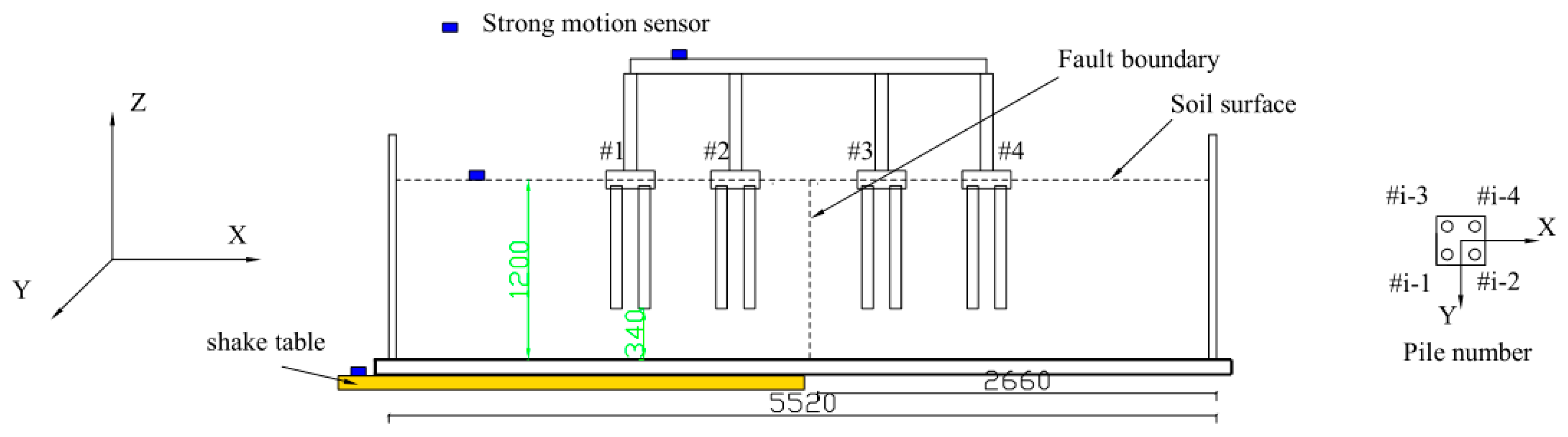
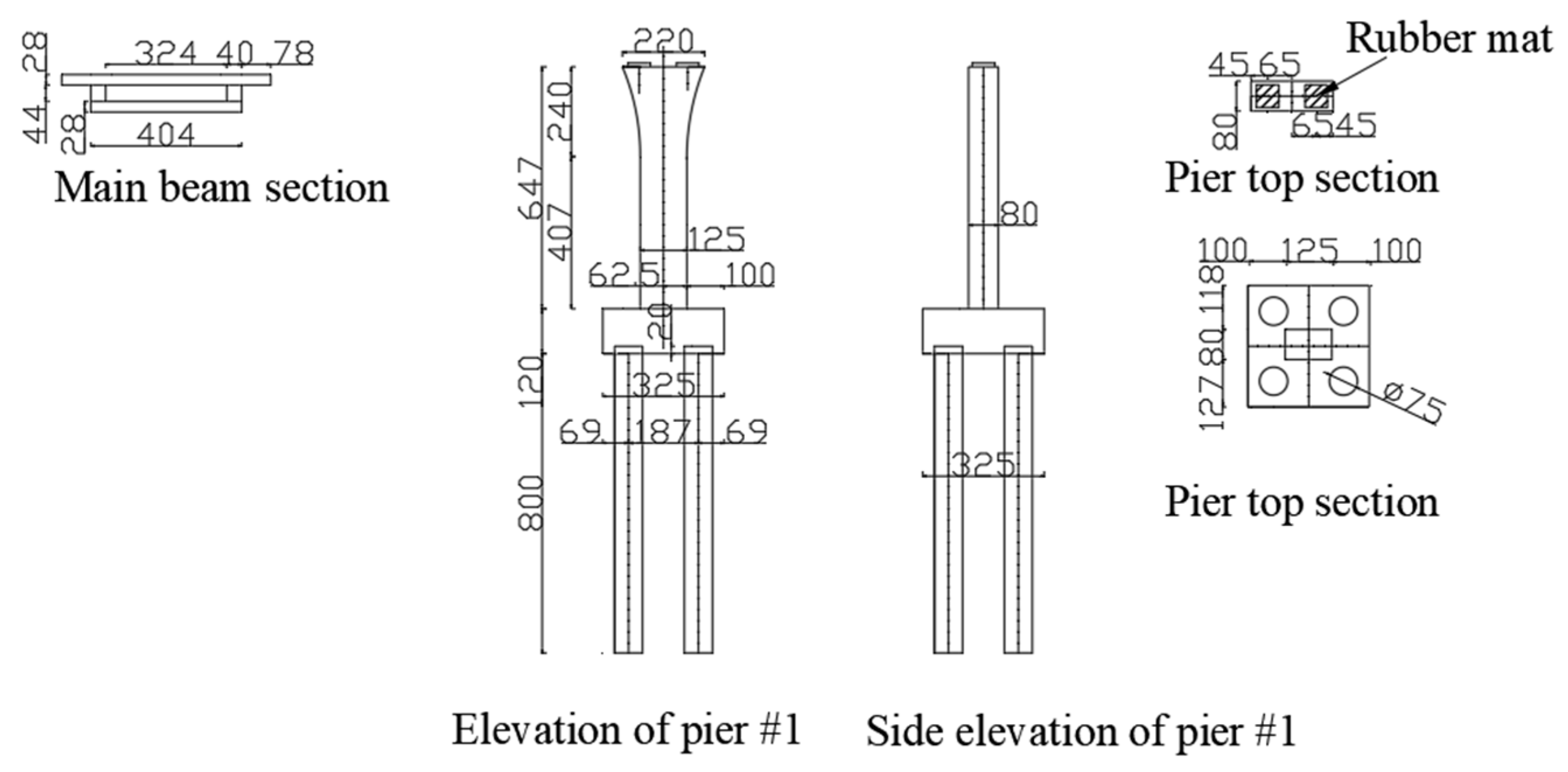
The bridge model

The test bridge model is made of polymethyl methacrylate with three spans of 700 + 975 + 700 mm, beam widths of 560 mm, and a height of 100 mm. The model is simplified as a single-chamber box structure. For the lower structure, both the middle piers (#2 and #3) and the side piers (#1 and #4) use vase piers with a height of 647 mm. The foundation piles of the bridge piers are 800 mm long with a diameter of 75 mm. The spacing between the pile bottom and the bottom of the box is about 340 mm, which is used to simulate friction piles. The piers #2 and #3 are fixed to the main beam to enhance the lateral stability of the bridge. The top of piers #1 and #4 are placed with rubber pads of 60 × 60 mm, and the center-to-center distance of the two supports is 130 mm, which provides torsional stability. Strong motion sensors are placed on the shake table, soil surface, and the bridge deck to record the system’s acceleration response. The schematic diagram of the model bridge and the arrangement on the shake table are shown in Figure 5, and a cross-section sketch of the bridge pier is shown in Figure 6.

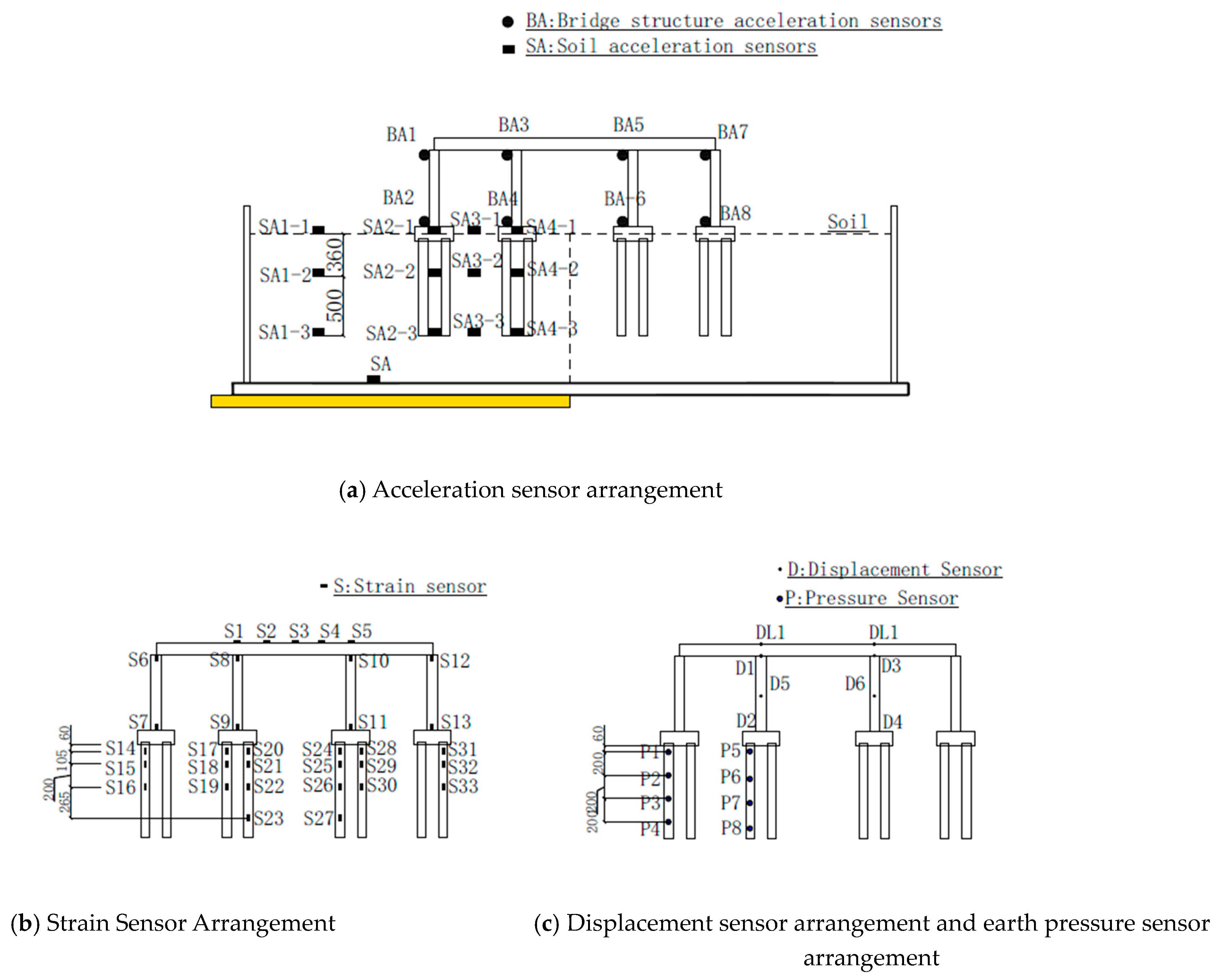
1.6. Instrument Deployments in the Test

The measurements carried out in the test include the accelerations of the model soil and bridge structure, strains of the model components, bridge-normal displacements of the structure, and the contact pressures between the model soil and piles, referring to the seismic failure mode of the cross-fault bridge structure and arrangement of measurements [29,30,31,32,33,34]. A total of 106 instruments are deployed, including 13 piezoelectric soil acceleration sensors, 24 three-component 941B structural acceleration sensors, 106 resistance strain gauges, 10 pull wire displacement sensors, and 16 piezoresistive soil pressure sensors. Figure 7 shows the locations of various instruments.

Different kinds of sensors, e.g., piezoelectric acceleration sensor, resistance structural strain sensor, piezoresistive soil pressure sensor, and displacement sensor, were used to record various parameters through a series of shaking table tests. The sensors included 21 acceleration sensors, 34 strain sensors, 8 soil pressure sensors, and 4 linear-wire displacement sensors, which were denoted as A, S, P and D, respectively. The arrangements of the sensors are shown in Figure 7.

To prevent the shift and tilt of acceleration sensors during the test, the sensors in soil should not be buried simply. When the filling soil was 150 mm higher than the location of the acceleration sensor, the shaft was dug, in which the bottom was tamped. Then, the acceleration sensor was buried, and the soil was put in by tamping. To prevent the damage of strain sensors on the piles, waterproof and wear-resistant treatments were performed. To ensure the measurement accuracy, the initial length linear-wire displacement sensor was around the intermediate range, and then, two ends of the sensors were fixed at the model structure and external steel frame outside the shaking table, separately [35,36,37,38,39].

1.7. Loading Scenarios for the Shaking Table Test

The purpose of the shaking table test in this paper is to study the effect of the interaction between the soil and pile on the seismic performance of a cross-fault bridge structure, and this study also focuses on the influence of input ground motion properties on the interaction between the soil and pile. Therefore, ground motion acceleration time-histories with different frequency characteristics and durations should be used as the input ground motion in the test [40,41].

In the test, three acceleration time-histories with permanent displacement are selected as input ground motions. The three ground motion acceleration time-histories and displacement time-histories, as shown in Figure 8, are as follows: (1) Modified Landers record, artificial acceleration time-histories based on a near-fault strong motion record from the 1992 Landers earthquake (Mw7.3) and designed permanent displacement, abbreviated in the text as L1; (2) Landers record, from the 1992 Landers earthquake (Mw7.2), abbreviated in the text as L2 [32]; (3) CHY024 record, from the 1999 Chi-Chi earthquake (Mw7.6), abbreviated in the text as C3. The differential displacement between the two sides of fault is used as the input to excite the bridge structure on one side of the fault, simulating the effect of ground motions on the seismic response of the cross-fault bridge structure. In order to investigate the changes in the model soil during the loading process and to prevent sudden failure of the structure, the seismic motion is carried out in the order of increasing peak ground motion, with peak ground displacements (PGD) of 0.83 cm, 1.67 cm, 3.33 cm, and 5.01 cm. Before the loading test of each ground motion input, white noise scanning is performed on the test structure system to measure its natural frequency. The loading scenarios are listed in

Table 2. Loading scenarios for the shaking table test.

Name	PGD (cm)
L1	0.83	1.67	3.33	5.01
L2	0.83	1.67	3.33	5.01
C3	0.83	1.67	3.33	5.01

.

2. Test Results and Interpretation

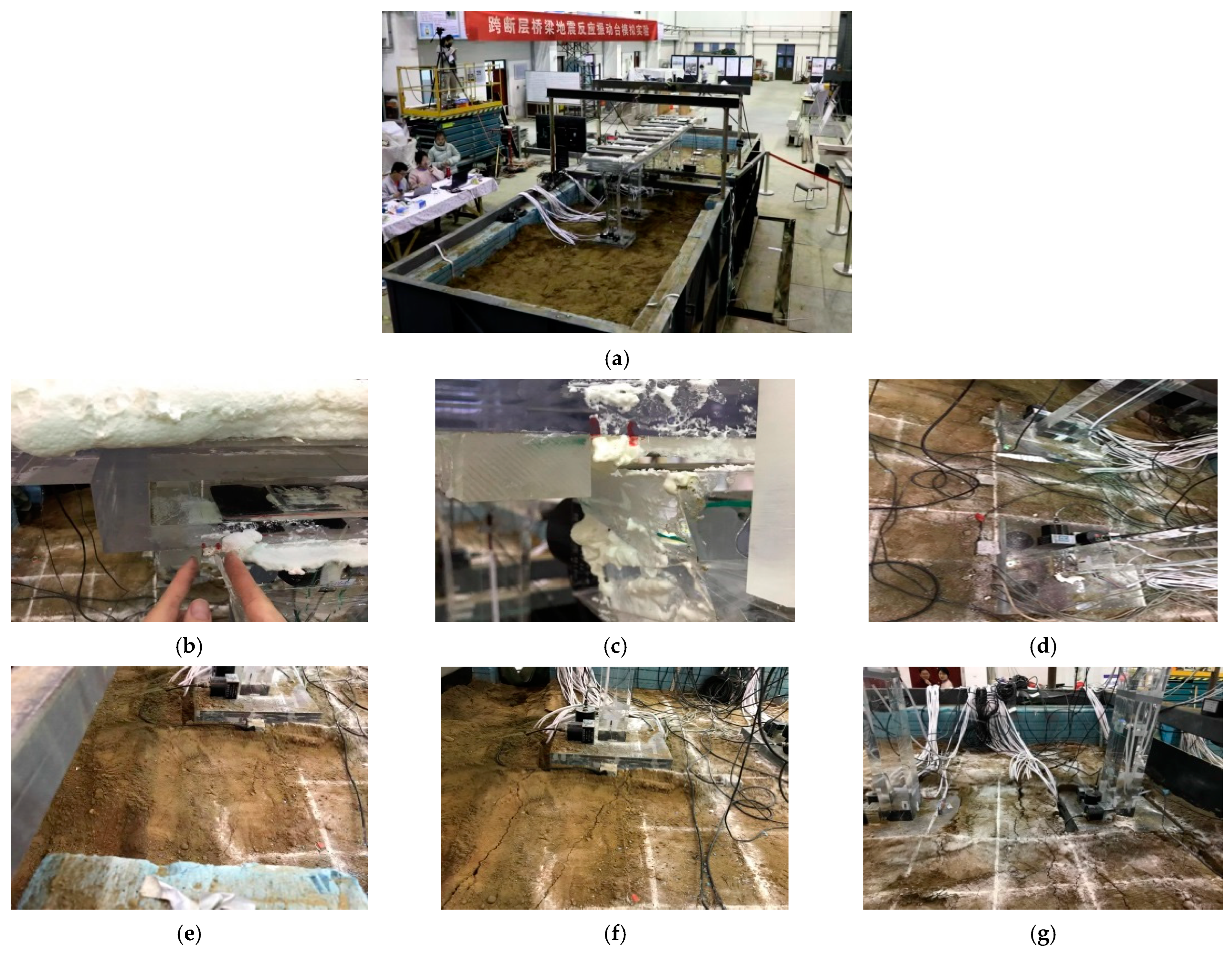
2.1. Visual Observations

For the loading scenario with a PGD of 0.83 cm, there is no obvious change for the soil and structure model. For the case with a PGD of 1.67 cm, there are slight cracks on the soil surface around each pier (#1–#4) and the abutment, as shown in Figure 9e. The structure is basically intact without obvious cracks. For the case with a PGD of 3.33 cm, there are obvious cracks on the soil surface around each pier (#1–#4) and the abutment, as shown in Figure 9f. The rubber bearings at the tops of piers #1 and #4 slide relative to the bridge deck, and there is a gradual sliding of the rubber bearing at the top of pier #1, as shown in Figure 9b. For the case with a PGD of 5.01 cm, there is an obvious separation between the soil and the abutment, as shown in Figure 9g. The top bearings of piers #1 and #4 slid significantly, and the piers are slightly tilted with an inclination angle of about 0.5°. After the test, there is no obvious damage or deformation to the bridge structure or the pile foundation.

2.2. Soil–Bridge Response to White Noise

Before the test, self-vibration characteristic testing was conducted on the test model using white noise input with a PGA of 0.05 g, and the acceleration time-history is recorded by the strong motion instruments deployed at the positions shown in Figure 9a. The Fourier spectrum of the white noise response recorded on the bridge deck is shown in Figure 10, from which the fundamental frequency of 2.3 Hz of the structure-foundation system model in the transverse direction is obtained.

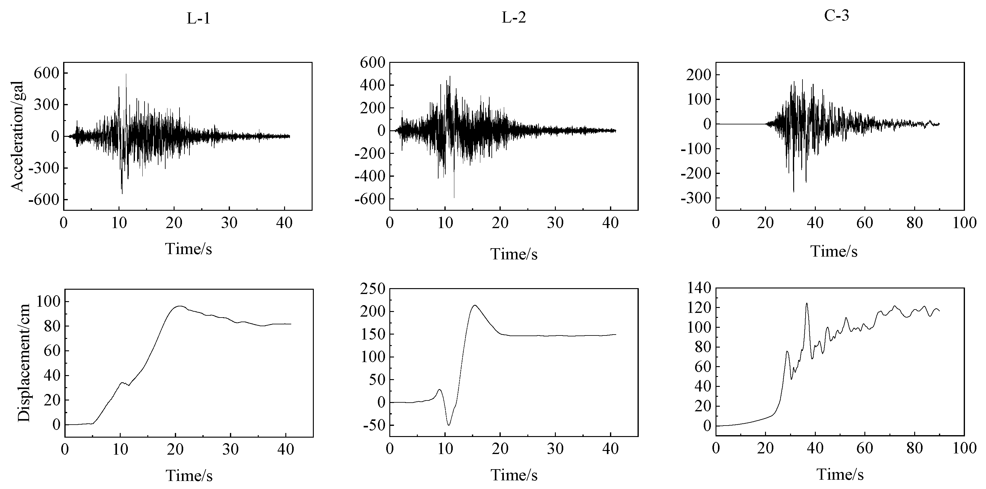
2.3. Inputs and Outputs of Shaking Table

In the shaking table test we employ displacement control input, and the loading scenarios are listed in Table 3. In the test, the interaction between the shaking table and the test model affects the control of the shaking table system, i.e., there is a certain difference between the controlled seismic input and the actual motion of the shaking table. For all loading scenarios in Table 3, the input and output of the shaking table are studied.

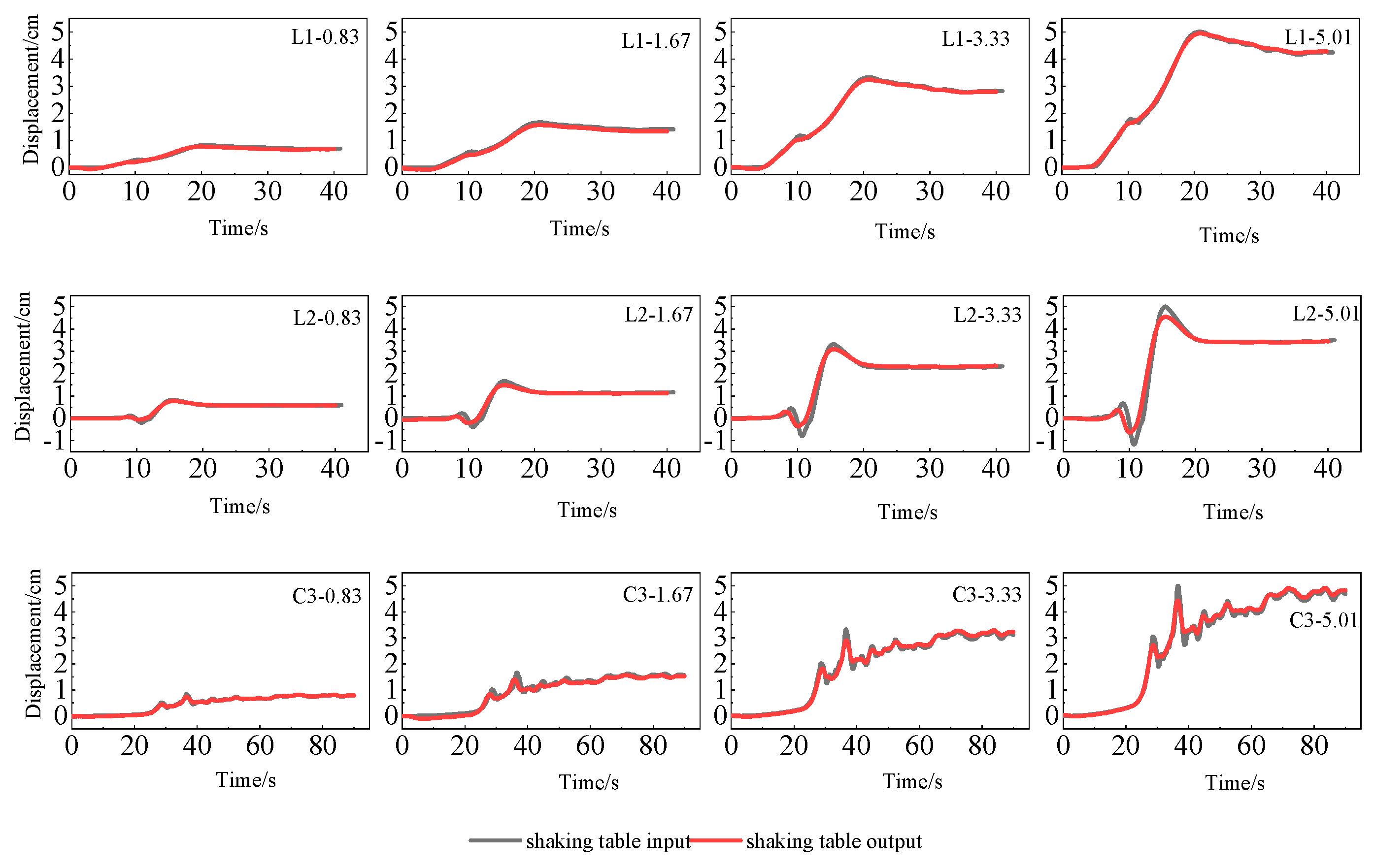
2.3.1. Displacement Output of the Shaking Table

A laser displacement sensor is installed on the shaking table to record the actual table motion during the test. Figure 11 compares the input and recorded seismic displacements on the table for all loading scenarios in the test, and

Table 4. Maximum torsion angles for different loading scenarios.

Loading Scenarios	PGD (cm)	L (cm)	Max D3 − D1 (cm)	$\mathit{\theta }$ (×10−3 rad)
L1	0.83	97.5	0.89	9.13
	1.67		1.77	18.15
	3.33		3.61	37.03
	5.01		5.43	55.69
L2	0.833		0.88	9.03
	1.67		1.68	17.23
	3.33		3.44	35.28
	5.01		4.84	49.64
C3	0.833		0.81	8.31
	1.67		1.60	16.41
	3.33		3.28	33.64
	5.01		4.91	50.36

lists the corresponding PGD values. In the Figure 11, the loading scenarios are abbreviated such that L1-0.83 represents the L1 record with an input PGD of 0.83 cm, L2-0.83 represents the L2 record with an input PGD of 0.83 cm, and C3-0.83 represents the C3 record with an input PGD of 0.83 cm. All ground motions are inputted in the transverse direction of the bridge. Figure 11 and Table 3 show that the difference between the actual shaking table motion and input motion designed for all loading scenarios are within a reasonable range, which meets the requirements of the test design.

Table 3. PGD values of designed and recorded input motions for all loading scenarios.

Designed PGD (cm)		0.83	1.67	3.33	5.01
Recorded PGD	L1	0.78	1.58	3.25	4.96
	L2	0.77	1.48	3.10	4.55
	C3	0.81	1.57	3.29	4.92

Table 3. PGD values of designed and recorded input motions for all loading scenarios.

Designed PGD (cm)		0.83	1.67	3.33	5.01
Recorded PGD	L1	0.78	1.58	3.25	4.96
	L2	0.77	1.48	3.10	4.55
	C3	0.81	1.57	3.29	4.92

In order to reflect the test results more accurately in the response analysis of the model test in the following sections, we use the actual recorded motion of the shaking table during the test as the input motion. Figure 12 shows the recorded acceleration time-histories, spectra, and the displacement time-histories of the shaking table for three selected input ground motions with a PGD of 1.67 cm.

2.3.2. Seismic Response of Bridge Structures

Summarizing the previous studies, the seismic response characteristics of the bridge across the fault are as follows: (1) the piers of the bridge across the fault are subjected to a larger torque; (2) in the direction of fault misalignment, the internal forces and displacements of the main girders, supports and piers, and piles on both sides of fault respond in the opposite direction; and (3) there are residual internal forces and displacements after an earthquake action [5,9,16]. Therefore, this section focuses on the analysis of structural displacement and strain responses to explore the reasonableness of the unilateral input test results.

2.3.3. Lateral Displacement and Torsional Response of the Main Beam

In order to investigate the lateral displacement and torsion of the main beam, we need to know the displacement difference between the two ends of the main beam. The piers #2 and #3 in the test model are both fixed, and therefore, we can assume that the displacements at the top are the same as those of the bridge deck. The data from the displacement gauges D1 and D3 are extracted to analyze the lateral displacement of the bridge deck at both ends when subjected to input motions in the transverse direction, and the maximum torsion angle of the bridge deck can be obtained. During the test, the bridge structure undergoes torsional motion, and the abutments generate torque because of the different displacements of D1 and D3. Based on the lateral displacement difference at both ends of the bridge deck, the torsion angle of the bridge deck can be calculated for different loading scenarios. The maximum lateral displacement difference of the bridge deck exceeds 2.5 cm. Figure 13 shows the diagram of the geometry, where L is the distance between the two ends of the bridge deck, and $\theta$ is the torsion angle.

Assuming that the bearing platform does not rotate during the test, the maximum torque at the base of each pier can be deduced from Equation (9) for each operating condition. The results are listed in Table 4. It can be seen that the greater the input PGD, the larger the torsion of the main beam. Under the same input PGD, there is no significant difference in the torsion angles of the bridge deck for L1, L2, and C3 input motion. When the input PGD is 5.01 cm, the maximum torsion angles are 55.69 × 10⁻³ rad, 49.64 × 10⁻³ rad, and 50.36 × 10⁻³ rad, respectively. Under the same input PGD, even if the high-frequency component of L2 is significantly higher than those of L1 and C3, the high-frequency component during the test does not have a significant impact on the lateral displacement and torsion of the main beam. This indicates that the differential ground displacement, i.e., the quasi-static component of the seismic motion, is the main factor causing the lateral displacement of the main beam in the cross-fault seismic bridge structure.

Assuming that the bearing platform does not rotate during the test, the height of the pier is $l$, and the cross-section of the pier is equivalent to a circular cross-section with a radius of $r$, the maximum tangential strain $\gamma$ at the base of each pier can be deduced from Equation (8), and the maximum torque at the base of the pier can be introduced from Equation (9), and $G$ is the shear modulus of the material.

$$\gamma =\frac{\theta r}{l}$$

(8)

$$T=G\gamma$$

(9)

In the test process, there is a phenomenon of separation of the bearing platform and soil, which proves that there is rotation of the bearing platform, and the relative torsion angle between the top and bottom of the pier is less than $\theta$. The maximum torque derived according to this method is able to envelope the most unfavorable situation of the bottom of the pier during the seismic design of the structure. The results of such calculation are significantly larger when studying the seismic response of the bridge across a fault. It is recommended to consider the effect of soil when conducting related studies.

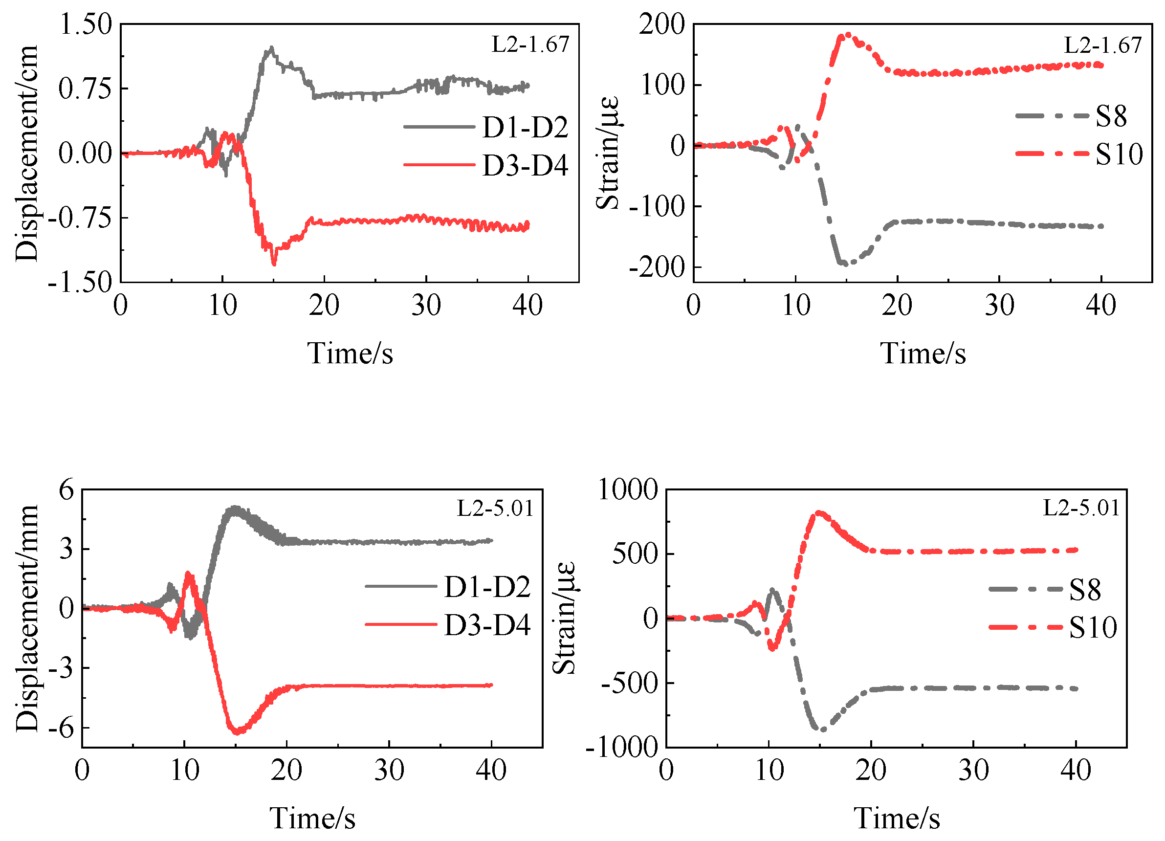
2.3.4. Displacement and Strain Response of the Main Beam on Both Sides of the Fault

Figure 14 shows the displacement time history of the main girder on both sides of the fault under T-0.83 and T-5.01 conditions. It can be seen that the displacement response of the main girder on both sides of the fault is in the opposite direction, which is in line with the basic characteristics of the seismic response of the bridge across the fault.

Figure 15 shows the strain time series at each measurement point of the main girder under T-0.83 and T-5.01 conditions. From the figure, it can be seen that the strain response at each location of the main girder on both sides of the bridge across the fault does not show symmetry like the displacement response. The displacement amplitude at each location is extracted for further study.

Figure 16 shows the strain amplitude of each observation point of the bridge deck under each working condition. When the input ground motion PGD is less than 1.67 cm, there is no obvious pattern in the strain response of each observation point of the bridge deck. When the input ground motion PGD is greater than 3.33 cm, the main strains at observation points of the bridge deck are larger at S2 and S4. The overall strain of the bridge deck does not reflect the symmetry, which leads to an unbalanced distribution of internal forces in the bridge structure during an earthquake, resulting in a reduction in the seismic resistance of the bridge structure. This is slightly different from the structural strain response caused by inputting equal and large inverse ground motion time histories on both sides of the fault [9]. In practical engineering, it is difficult to make the ground motions on both sides of the fault equal and inverse; therefore, which one of these input methods is more realistic to respond to the earthquake situation needs to be further discussed.

Figure 17 compares the S2 and S4 strain amplitudes of PGD 1.67 and 5.01 under each loading scenario, and when PGD is the same, the S4 strain amplitude is basically the same for each ground motion, and there is an obvious difference at S2. This indicates that the dynamic effect of ground motion has a significant contribution to the tangential strain of the main beam. The dynamic effect of ground motion needs to be paid attention to when analyzing the tangential strain or internal force seismic response of the main beam.

Figure 18 shows the relative displacement time histories of the top of pier #2 and pier #3 on both sides of the fault relative to the bottom of the pier and the strain time histories at the top of the pier. The displacement direction is in the transverse bridge direction, and the strain is in the vertical strain direction. From the figure, we can see that the displacement time histories and strain time histories of two piers are in opposite directions, and there is a certain symmetry. When the response stops, there exists the residual displacement and strain, and there is relative motion between the top and bottom of the pier, which can lead to the tilting of piers. Due to the presence of permanent displacement in the input seismic motion, the soil surface also has permanent displacement after the response stops, and the bridge structure does not return to its equilibrium position before testing. This results in piers maintaining an inclined state when the response motion ends, which can be extremely harmful to the bridge structure.

Table 5. Maximum instantaneous inclination angles of piers #2 and #3 for different loading scenarios.

Loading Scenarios	PGD (cm)	L (cm)	2#Max D3 − D1 (cm)	$\mathit{\theta }$ (×10−3 rad)	3#Max D3 − D1 (cm)	$\mathit{\theta }$ (×10−3 rad)
L1	0.83	64.7	0.12	1.8	0.12	1.8
	1.67		0.21	3.2	0.2	3.1
	3.33		0.36	5.6	0.41	6.3
	5.01		0.49	7.6	0.64	9.8
L2	0.833		0.13	2	0.14	2.1
	1.67		0.21	3.2	0.23	3.5
	3.33		0.41	6.3	0.41	6.3
	5.01		0.56	8.6	0.63	9.7
C3	0.833		0.12	1.8	0.12	1.9
	1.67		0.22	3.4	0.22	3.4
	3.33		0.39	6.0	0.41	6.3
	5.01		0.51	7.8	0.63	9.7

provides the maximum instantaneous inclination angles of piers #2 and #3 for different loading scenarios, and

Table 6. Maximum permanent inclination angles of piers #2 and #3 for different loading scenarios.

Loading Scenarios	PGD (cm)	L (cm)	2#Max D3 − D1 (cm)	$\mathit{\theta }$ (×10−3 rad)	3#Max D3 − D1 (cm)	$\mathit{\theta }$ (×10−3 rad)
L1	0.83	64.7	0.10	1.5	0.12	1.8
	1.67		0.17	2.6	0.2	3.1
	3.33		0.36	5.6	0.32	4.9
	5.01		0.49	7.5	0.52	8.0
L2	0.833		0.10	1.5	0.10	1.5
	1.67		0.15	2.3	0.18	2.8
	3.33		0.25	3.9	0.24	3.7
	5.01		0.56	8.7	0.48	7.4
C3	0.833		0.11	1.7	0.11	1.7
	1.67		0.21	3.2	0.21	3.2
	3.33		0.32	4.9	0.34	5.2
	5.01		0.51	7.9	0.59	9.1

lists the permanent inclination angles. It can be seen that the larger the input PGD, the larger the inclination angle of the bridge pier. The inclination angles of piers #2 and #3 for the same input PGD are roughly the same in magnitude, but in opposite directions, with a maximum instantaneous inclination angle of 9.8 × 10⁻³ rad and a maximum permanent inclination angle of 9.1 × 10⁻³ rad. When examining the seismic response of a cross-fault bridge structure, the maximum instantaneous inclination angle of the bridge pier and the permanent inclination angle of the bridge pier after the response motion ends should be considered separately.

To further explore the torsional response characteristics of the bridge structure, this study introduces the structural torsional enlargement factor (STEF) defined as the ratio of the torsional angle recorded at the same measuring point with different PGD actions to the torsional angle recorded when the PGD is 0.83 cm. Figure 19 shows the structural torsional enlargement coefficient at different locations under different loading scenarios. From the figure, it can be seen that the instantaneous maximum torsional enlargement factors for the main girder, pier 2#, and pier 3# increase linearly. There is no nonlinear change in the structure. This indicates that the bridge model has better seismic performance, and the simply supported girder design on both sides of the main girder can increase the degree of freedom of the bridge structure, thereby reducing the torsional damage of the bridge structure. However, the enlargement factors of the permanent torsional angle of pier 2# and pier 3 showed a nonlinear change with the increase in the PGD. This indicates that the permanent displacement of ground motion is more serious for the torsional damage of the bridge relative to the PGD. In the structural seismic design of cross-fault bridges, the effect of seismic permanent displacement on the seismic response of bridge structures must be considered.

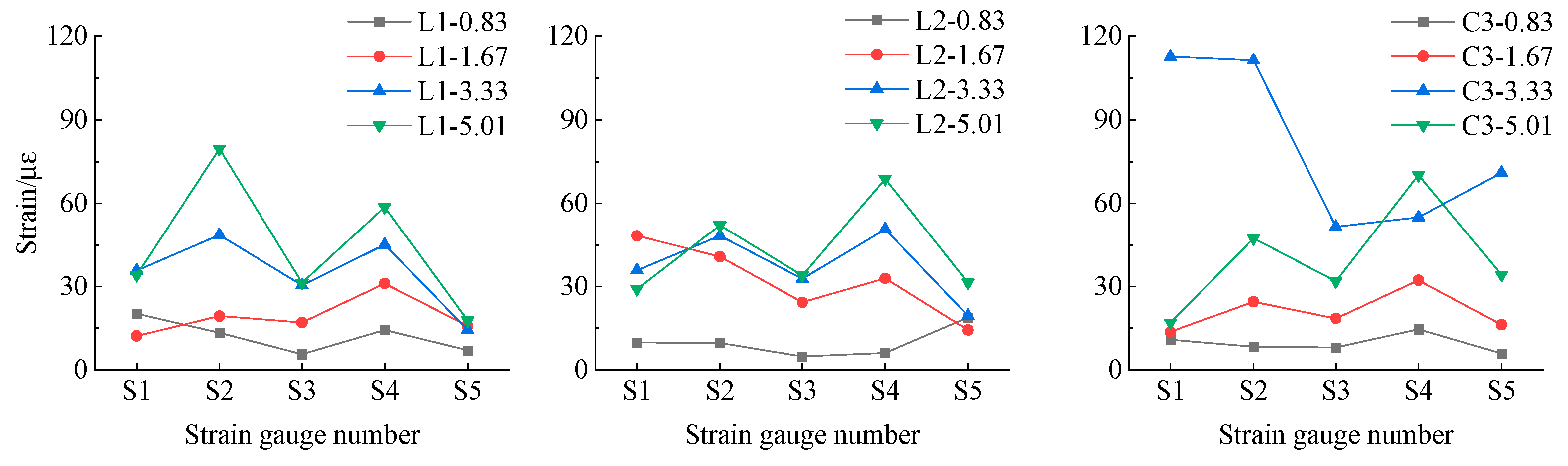
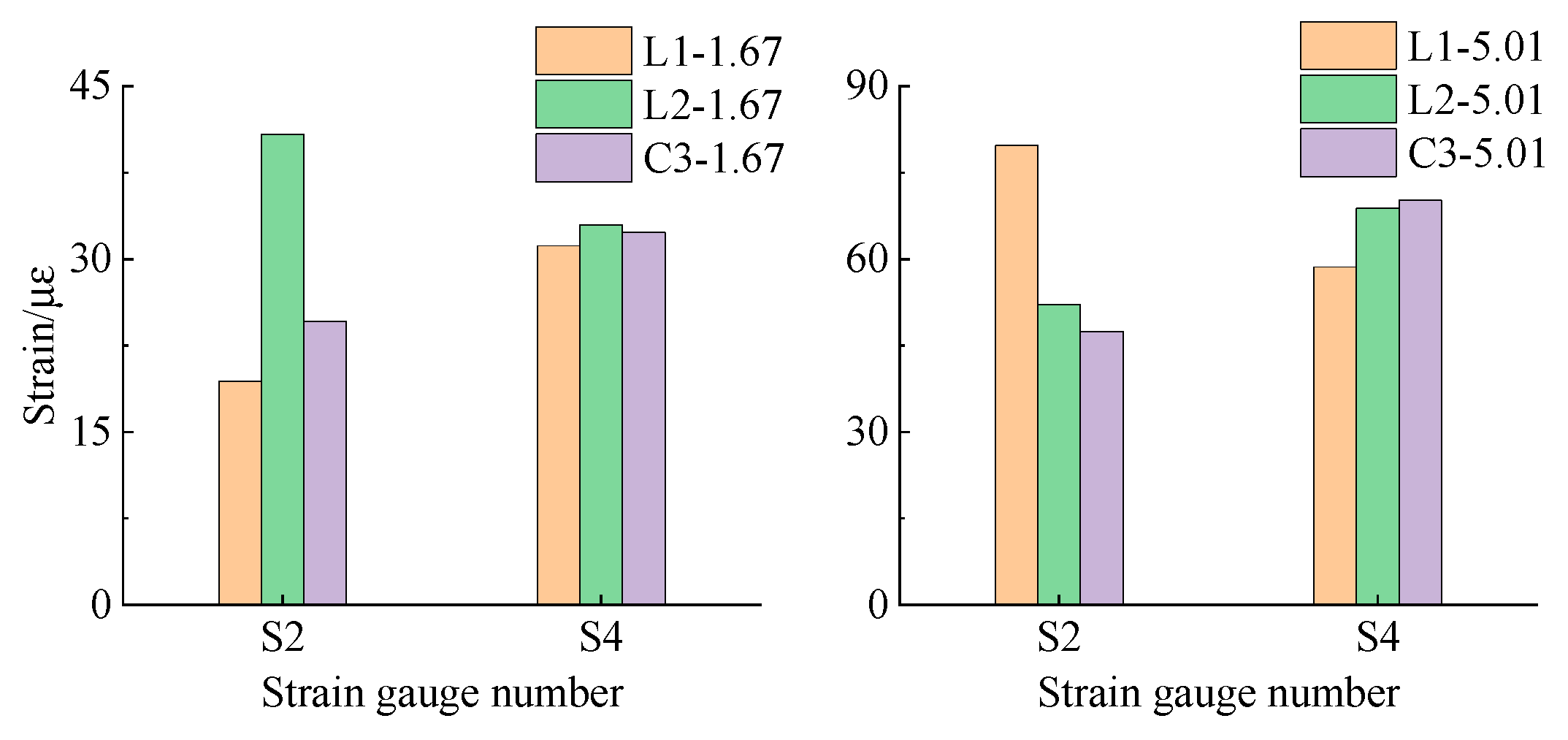
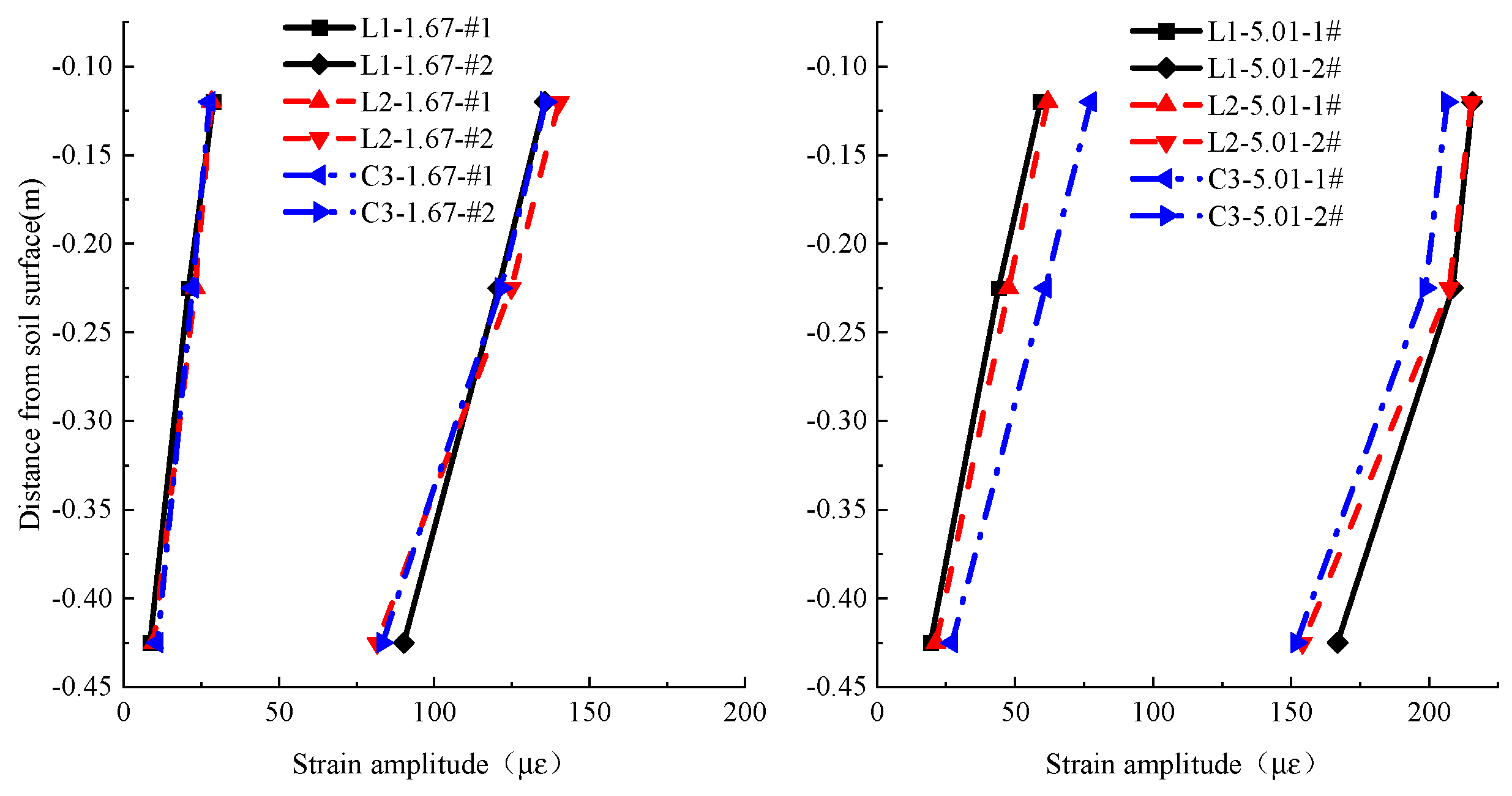
2.3.5. Comparison of Strain Response of Pile Body on Both Sides of the Fault

Figure 20 illustrates the relative displacement time histories at the top of pier #2 and pier #3 on both sides of the fault relative to the bottom of the pier and the strain time histories at the top of the pier. The displacement direction is in the transverse bridge direction, and the strain is in the vertical strain. From the figure, we can see that the displacement time course and strain time course of the two piers are in opposite directions, and there is a certain symmetry. When the response stops, there are the residual displacement and strain, and there is relative motion between the top and bottom of the pier, which can lead to the tilting of piers. To investigate the deformation of the pile foundation, we analyze the strain records from the strain gauges SA2-1 to SA2-3 on pile 1 and SA4-1 to SA4-3 on pile 2 for different loading scenarios. The peak strain amplitudes along the height of the pile foundation are shown in Figure 21.

Figure 21 shows that with an increase in the input PGD, the overall trend is an increase in the strain at the pile foundation. Under the same loading scenarios, the strain amplitude at the top of pile is the largest, while that at the bottom, it is the smallest. The strain of the pile decreases with the depth increasing, which is consistent with the actual earthquake damage pattern of bridges, because the top of the pile foundation is fixed to the bearing platform, while the bottom is basically in a free state. Under the same input PGD for L1, L2, and C3, the strains are basically the same at different locations of the pile foundation. We know that under the same input PGD, the high-frequency component of L2 is significantly larger than those of L1 and C3. However, in this test, there is no significant difference in the strain amplitude at the pile foundation due to the different high-frequency components of the input motions. This indicates that peak displacement, i.e., the quasi-static effect of input motion, is the main factor affecting the strain response of the pile foundation. In Figure 22, we can also see that under the same input PGD, the strain response at the foundation of pier #2 near the fault is much larger than that of pier #1. In the practical engineering design of cross-fault bridges, the seismic response of pile foundations near the fault should be emphasized. It is recommended that seismic isolation bearings and other seismic engineering techniques be used to increase the freedom of bridge piers and pile foundations and reduce their strain responses.

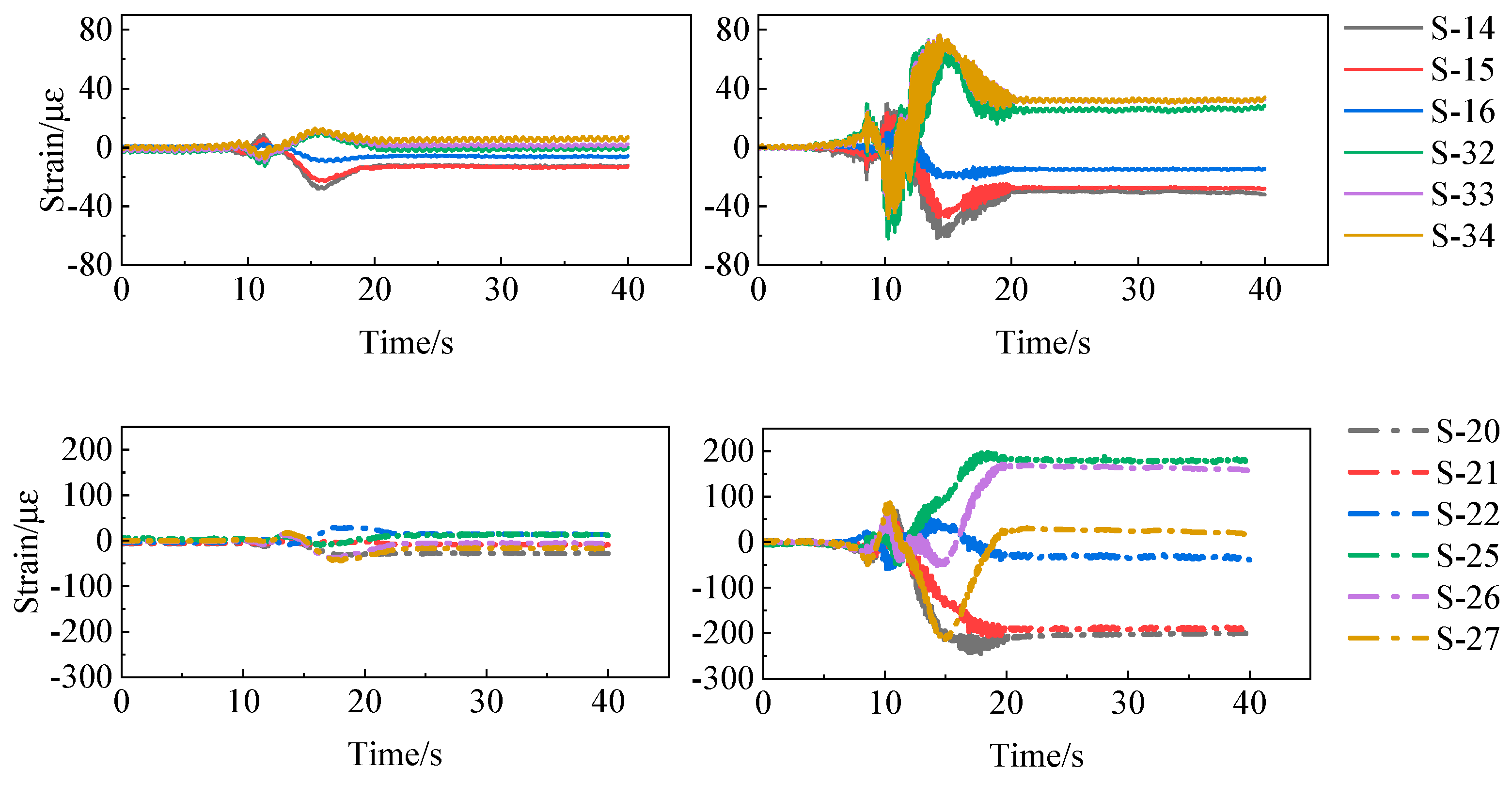
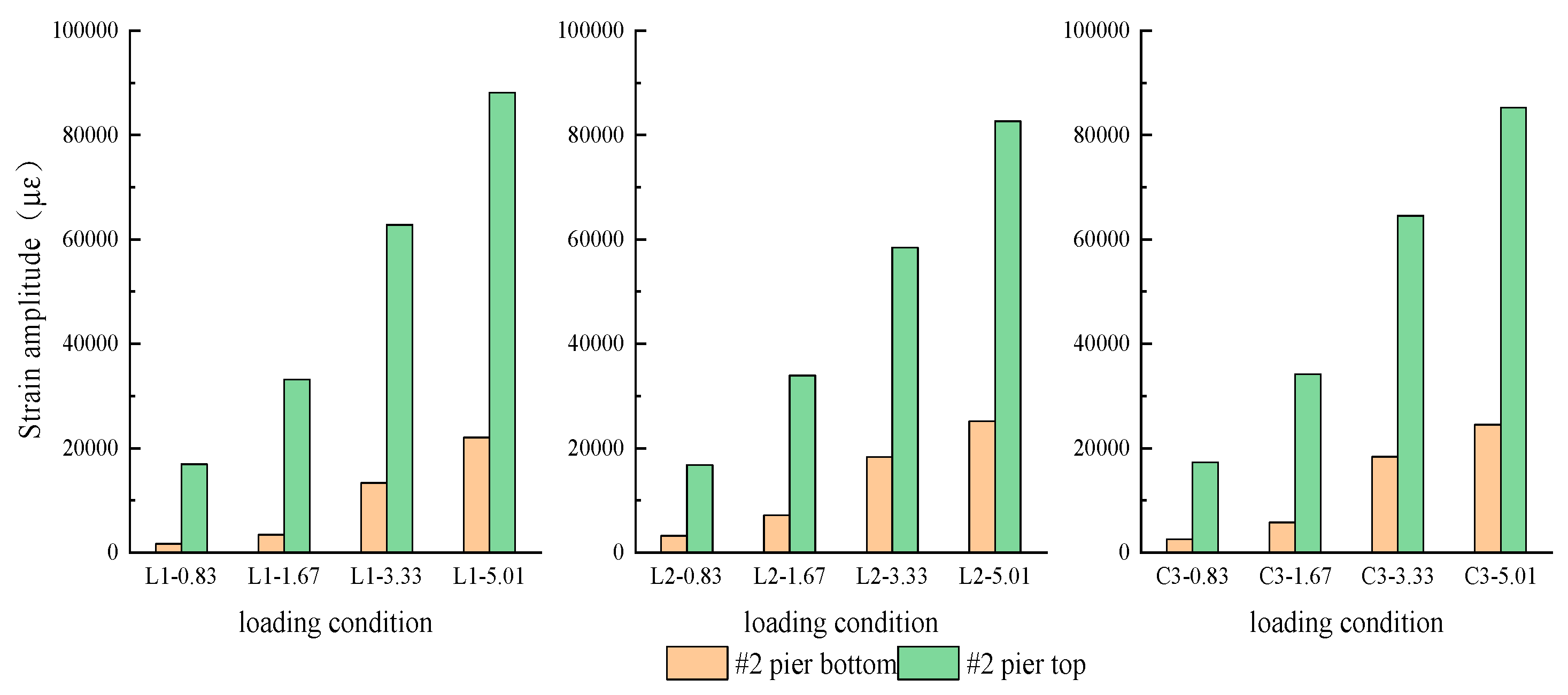
2.3.6. Pier Strain Variation

Based on the strain data at the bottom of the four piers and the top of piers #2 and #3, the distribution pattern of the transverse strains at the bottom of the piers can be analyzed. The results of strain amplitude measurements are listed in

Table 7. Maximum strains at the tops and bottoms of piers.

Location	Name	$\mathbf{Strain} \mathbf{Amplitude} (\mathit{\mu }\mathit{\epsilon }$)
		0.83 cm	1.67 cm	3.33 cm	5.01 cm
#1 pier bottom (SDX-5)	L1	1363	1407	1635	5409
	L2	1614	1562	2359	7691
	C3	1478	1665	14,046	9996
#2 pier top (SDX-2)	L1	16,874	33,158	62,827	88,085
	L2	19,078	35,636	62,735	86,981
	C3	17,282	34,192	64,535	85,272
#2 pier bottom (SDX-6)	L1	1623	3351	13,294	22,033
	L2	2187	4821	16,271	26,465
	C3	2502	5751	18,362	24,473
#3 pier top (SDX-3)	L1	13,743	30,013	59,490	82,828
	L2	16,768	33,903	58,435	82,691
	C3	14,875	31,690	76,204	79,618
#3 pier bottom (SDX-7)	L1	2621	4795	15,954	21,013
	L2	3163	7143	18,282	25,138
	C3	3439	7244	16,401	23,822
#4 pier bottom (SDX-8)	L1	1646	2539	4828	8521
	L2	1938	2515	8674	14,724
	C3	1684	2510	51,742	10,435

.

Figure 22. Strains at the bottoms of piers for different loading scenarios.

Figure 22. Strains at the bottoms of piers for different loading scenarios.

Figure 23 shows that with the increase in the input PGD, the strains at the top and bottom of the pier exhibit an increasing trend, with a maximum strain of 88,058 $\mu \epsilon$. Under the same input PGD, the strains of the pier for L1, L2, and C3 are basically the same. In Figure 18, the comparison of the strains at the bottom of four piers shows that the strains at the bottom of piers #2 and #3 are much larger than those at the bottom of piers #1 and #4. This is because the tops and bottoms of piers #2 and #3 are in a fixed state and have larger bending moments, while piers #1 and #4 have obvious displacement from the main beam during testing, which greatly reduces the strains at the latter two piers. From the strain data of piers #2 and #3 in Table 5, it can be seen that the strain at the top of each pier is significantly larger than the strain at the bottom. Compared with the strain amplitude of the pile foundation mentioned earlier, the strain of the pier is generally larger than that of the pile foundation, indicating that the soil has an effect of resisting the motion of the pile foundation. This also indicates that the participation of soil could reduce the seismic response of the structure.

To summarize the test results of the seismic response of the bridge structure, the bridge across the fault is subjected to torsion at the piers during the seismic motion, and the strain and displacement responses of piers and piles on both sides of the fault in the direction of fault misalignment are in opposite directions. The strain and displacement responses of piers and piles are mainly affected by the quasi-static effect of ground motion. The displacement response of the main beam on both sides of the fault is opposite, and there are residual internal forces and displacements after the seismic motion ends. The test results indicate that the seismic response characteristics of the bridge across the fault are basically simulated by the shaking table test in this study; therefore, the one-side input method proposed in this shaking table test is suitable for the seismic response test of the bridge across the fault.

3. Effects of Soil–Structure Interaction on the Acceleration Response of Soils and Bridge Structures

In order to study the acceleration response characteristics of the soil and bridge structure, this study introduces the peak acceleration amplification factor (PAAF) defined as the ratio of the peak acceleration recorded at each measuring point to the peak acceleration on the shaking table [40,42]. The peak acceleration amplification factors at the sensor location in soil (Figure 7a) for different loading scenarios are shown in Figure 24.

For the variation trend of amplification factors at comparative positions SA1, SA2, SA3, and SA4, it can be observed that the variation in PAAF in the free soil far away from the piers is significantly greater than other locations, such as those between piles and between piers. At a depth of −0.86 m in the free soil, the PAAF is generally around 0.1, while at locations, such as SA2, SA3, and SA4, the PAAF is greater than 0.2 due to the influence of the structure. At the free surface of oil, the PAAF is generally around 1.5, while at locations, such as SA2, SA3, and SA4, it is less than 1.2 due to the influence of the structure. This indicates that the friction and collision between the soil and structure cause the variation in PAAF to be smaller when the seismic wave propagates in the vicinity of the structure than in the free soil far away from the structure. With the increase in PGD, the amplification factor tends to be the same at −0.36 m for positions, such as SA1, SA2, SA3, and SA4. This is due to the fact that as the input PGD of seismic motion increases, separation occurs between the pile and soil, weakening the soil–structure interaction. The absence of this phenomenon at −0.83 m is due to the deeper burial depth and no separation of the pile and soil. The absence of this phenomenon on the soil surface is also due to the fact that the soil near the structure was affected by the soil–structure interaction. This results in different acceleration amplification coefficients at the soil surface.

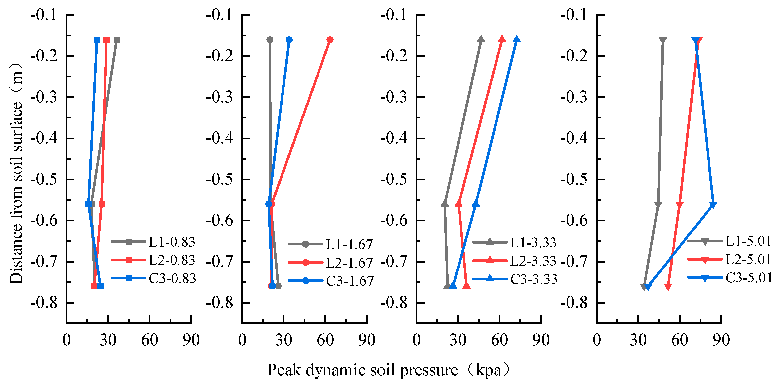
4. Variation in Dynamic Soil Pressure near the Pile

The difference in medium properties and motion characteristics between the pile foundation and soil results in dynamic soil pressure between them. Taking pile #1 as an example, we analyze the dynamic soil pressure distribution by extracting the soil pressure at sensor locations T-X-1, T-X-2, and T-X-4 on the pile when the seismic motion is inputted in the X direction. The peak dynamic soil pressures along pile #1 for different loading scenarios are shown in Figure 22.

Figure 25 shows that the dynamic soil pressure increases with the increase in the input PGD. The maximum dynamic soil pressure is at the top of the pile, and with the increasing depth, the dynamic soil pressure decreases. When the input PGD is small, the increasing trend is relatively small. This is because when the input motion is small, there is no separation between the pile and soil at the contact surface. With the increase in the input PGD, the soil deformation increases. Closer to the top of pile, the relative motion between the structure and soil is more intense, and the pile and soil gradually separate, resulting in an increase in the dynamic soil pressure.

For the L1 and C3 with a PGD of 3.33 cm or more, the increasing trend of the dynamic soil pressure at the top of the pile is more obvious. For the L2 with a PGD greater than 1.67 cm, the increasing trend of the dynamic soil pressure at the top of the pile is significantly increased. This is because the L2 contains more high-frequency components than the L1 and C3. Therefore, we can infer that the more high-frequency components of the input motion, the more obvious the increasing trend in the dynamic soil pressure.

5. Conclusions

The near-fault seismic ground motions are characterized by large acceleration, velocity and displacement, a long period, and permanent displacement, which greatly increases the complexity of the seismic response of the cross-fault bridge structure and leads to severe damage. In the shaking table test for a cross-fault bridge model, in order to simulate the effect of the ground motion difference on both sides of the fault, the differential displacement between the two sides of the fault are applied as the input motion on one side of the bridge. The feasibility of this scheme proposed is confirmed through numerical simulation. Three time-displacement histories derived from ground motion acceleration records are utilized to construct four distinct loading scenarios with varying peak ground displacements. The findings from numerous instruments located at different sites are examined to explore how the magnitude of displacement and the frequency content of seismic motions affect the seismic response of the cross-fault bridge structure. The test results show the following:

• The one-side input method proposed in this study can reproduce the different ground motions and permanent displacements on both sides of fault. This method can effectively simulate the ground motion on both sides of the fault. This provides a reference for conducting similar tests in the future.
• During the shaking table test, the actual shaking table motion is essentially the same as the input motion designed. But due to the limitations in the shaker’s own performance, it results in a missing structural dynamic response when using peak displacement as the input control. Since the seismic response of the bridge across the fault mainly comes from the proposed static component of ground shaking, the missing dynamic component has little effect on the test results. Additional calculations of the structural dynamic response of the bridge can be made subsequently via numerical simulation.
• The seismic behavior of a cross-fault bridge is markedly influenced by both quasi-static and dynamic effects. The quasi-static effect is the main factor that affects the acceleration amplification factor of the soil–structure system, the bridge’s displacement, torsion, and strain responses. Furthermore, the dynamic effect has a significant influence on the dynamic soil pressure.
• The highest strain is observed at the pile’s top, with the lowest at the bottom, indicating that strain decreases with depth from the top to the bottom of the pile. The peak displacement of the input seismic motion is the main factor that affects the strain response of the bridge structure. The strain response of the pile foundation close to the fault is considerably larger than that further away from the fault. For the seismic design of cross-fault bridges in practical engineering, it is recommended to focus on the seismic response of the pile foundation near the fault and to use seismic isolation bearings and other engineering techniques to increase the freedom of the pier and pile foundation and reduce their strain responses. The strain of the pier is generally greater than that of the pile foundation, indicating that the soil has an effect of resisting the motion of the pile foundation.
• The permanent displacement of ground motion has a greater impact on the torsional response of bridge structures compared to the PGD. Considering the special characteristics of the seismic response of cross-fault bridge structures, the maximum instantaneous inclination angle and the permanent inclination angle of the pier after the earthquake should be considered separately during the structural seismic design.
• The difference in seismic motions on both sides of the fault has a significant and complicated effect on the seismic response of the cross-fault bridge structure. The use of near-fault seismic motions with different characteristics may lead to significantly different seismic responses of the bridge structure. When analyzing the bridge structure that crosses active faults, the large deformation caused by fault slip and surface rupture should be fully considered to evaluate the seismic performance of the bridge.

References

- Hui, Y.X.; Tai, Y.J.; Wang, K.H.; Zhang, S. Discussion about Earthquake Resistance of the Bridges Crossing the Active Fault. China Earthq. Eng. J. 2017, 39, 870–875. [Google Scholar]
- European Committee for Standardization. Eurocode8: Design of Structures for Earthquake Resistance. Part 5: Foundation, Retaining Structures, and Geotechnical Aspects; EVN; European Committee for Standardization: Brussels, Belgium, 1998; pp. 14–20. [Google Scholar]
- Caltrans. Bridge Design Practice Manual; California Department of Transportation: Sacramento, CA, USA, 2012.
- Caltrans. Seismic Design Criteria: Version 1.9; California Department of Transportation: Sacramento, CA, USA, 2020.
- Yang, S.; Mavroeidis, G.P. Bridges crossing fault rupture zones: A review. Soil Dyn. Earthq. Eng. 2018, 113, 545–571. [Google Scholar] [CrossRef]
- Wang, N.; Elgamal, A.; Lu, J. Assessment of the Samoa Channel Bridge-foundation seismic response. Soil Dyn. Earthq. Eng. 2018, 108, 150–159. [Google Scholar] [CrossRef]
- Goel, R.K.; Chopra, A.K. Role of shear keys in seismic behavior of bridges crossing fault-rupture zones. Bridge Eng. 2008, 13, 398–408. [Google Scholar] [CrossRef]
- Deng, Q.D. Active Tectonics in China. Geol. Rev. 1996, 42, 295–299. [Google Scholar]
- Saiidi, M.S.; Vosooghi, A.; Choi, H.; Somerville, P. Shake Table Studies and Analysis of a Two-Span RC Bridge Model Subjected to a Fault Rupture. J. Bridg. Eng. 2014, 19, 1943–5592. [Google Scholar] [CrossRef]
- Tseng, W.S.; Penzien, J. Seismic analysis of long multiple-span highway bridges. Earthq. Eng. Struct. Dyn. 1975, 4, 1–24. [Google Scholar] [CrossRef]
- Murono, Y.; Miroku, A.; Konno, K. Experimental Study on Mechanism of Fault-Induced Damage of Bridges; Technical Report; Chuo Fukken Consultants: Osaka, Japan, 2005. [Google Scholar]
- Roussis, P.C.; Constantinou, M.C.; Erdik, M.; Durukal, E.; Dicleli, M. Assessment of Performance of Seismic Isolation System of Bolu Viaduct. J. Bridg. Eng. 2003, 8, 182–190. [Google Scholar] [CrossRef]
- Park, S.; Ghasemi, H.; Shen, J.; Somerville, P.; Yen, W.; Yashinsky, M. Simulation of the seismic performance of the Bolu Viaduct subjected to near fault ground motions. Earthq. Eng. Struct. Dyn. 2004, 33, 1249–1270. [Google Scholar] [CrossRef]
- Güney, D.; Acar, M.; Özlüdemir, M.; Çelik, R. Investigation of post-earthquake displacements in viaducts using Geodetic and Finite Element Methods. Nat. Hazards Earth Syst. Sci. 2010, 10, 2579–2587. [Google Scholar] [CrossRef]
- Hui, Y.X.; Wang, K.H. Study of Seismic Response Features of Bridge Crossing Faults. Bridge Constr. 2015, 45, 70–75. [Google Scholar]
- Hui, Y.X.; Wang, K.H. Earthquake motion input method for bridges crossing fault based on multi-support excitation displacement input model. J. Southeast Univ. 2015, 45, 557–562. [Google Scholar]
- Du, X.L.; Han, Q.; Li, X.Z.; Li, L.Y.; Chen, S.F.; Zhao, J.F. The Seismic Damage of Bridge in the 2008 Wenchuan Earthquake and Lessons from Its Damage. J. Beijing Univ. Technol. 2008, 34, 1270–1279. [Google Scholar]
- Zong, Z.H.; Lin, Y.Z.; Li, Y. Research Advances of across-fault Ground Motions and Their Effects on Bridge Structures. China J. Highw. Transp. 2023, 36, 80–96. [Google Scholar] [CrossRef]
- Lu, C.H.; Liu, K.Y.; Chang, K.C. Seismic performance of bridges with rubber bearings: Lessons learnt from the 1999 Chi-Chi Taiwan earthquake. J. Chin. Inst. Eng. 2011, 34, 889–904. [Google Scholar] [CrossRef]
- Goel, R.K.; Chopra, A.K. Nonlinear Analysis of Ordinary Bridges Crossing Fault-Rupture Zones. J. Bridg. Eng. 2009, 14, 216–224. [Google Scholar] [CrossRef]
- Goel, R.K.; Chopra, A.K. Linear Analysis of Ordinary Bridges Crossing Fault-Rupture Zones. J. Bridg. Eng. 2009, 14, 203–215. [Google Scholar] [CrossRef]
- Han, Q.; Du, X.; Liu, J.; Li, Z.; Li, L.; Zhao, J. Seismic damage of highway bridges during the 2008 Wenchuan earthquake. Earthq. Eng. Eng. Vib. 2009, 8, 263–273. [Google Scholar] [CrossRef]
- Lin, Y.; Zong, Z.; Bi, K.; Hao, H.; Lin, J.; Chen, Y. Experimental and numerical studies of the seismic behavior of a steel-concrete composite rigid-frame bridge subjected to the surface rupture at a thrust fault. Eng. Struct. 2019, 205, 110105. [Google Scholar] [CrossRef]
- Wang, Z.; Dueñas-Osorio, L.; Padgett, J.E. Influence of soil-structure interaction and liquefaction on the isolation efficiency of a typical multispan continuous steel girder bridge. J. Bridge Eng. 2014, 19, A4014001. [Google Scholar] [CrossRef]
- Zhang, Z.; Song, C.; Li, X.; Lan, R. Comparative study on the small radius curved bridge and simplified models by shaking table tests. J. Bridge Eng. 2021, 26, 04021039. [Google Scholar] [CrossRef]
- Xu, B.W. Shaking Table Test Studying Large-Scale Soil-Pile-Complex Structure Interaction; Tianjin University: Tianjin, China, 2009. [Google Scholar]
- Jiang, X.L.; Xu, B.W.; Jiao, Y. Analysis of shaking table test of large-scale soil-pile-complex structure interaction. China Civ. Eng. J. 2010, 43, 98–105. [Google Scholar] [CrossRef]
- Chen, G.; Chen, S.; Zuo, X.; Du, X.; QI, C.; Wang, Z. Shaking-table tests and numerical simulations on a subway structure in soft soil. Soil Dyn. Earthq. Eng. 2015, 76, 13–28. [Google Scholar] [CrossRef]
- LINSemih, E.; Murat, D. Effect of dynamic soil–bridge interaction modeling assumptions on the calculated seismic response of integral bridges. Soil Dyn. Earthq. Eng. 2014, 66, 42–55. [Google Scholar] [CrossRef]
- Zhang, F.; Li, S.; Wang, J.Q. Numerical analysis on seismic response of bridges crossing normal fault rupture zone. J. Build. Struct. 2022, 43, 205–216. [Google Scholar] [CrossRef]
- Guan, Z.G.; You, H.; Guo, H. Responses of Cable-Stayed Bridge Transversely Isolated with Elasto-Plastic Clabe Pairs and Fluid Viscous Damper Subjected to Near Fault Ground Motions. J. Tongji Univ. 2016, 44, 1653–1659. [Google Scholar]
- Li, X.J.; Sun, J.Y.; Wang, N.; Rong, M.S.; Dong, Q. Analysis of Seismic Response of Bridge across Earthquake Fault with Different Input Modes of Seismic Action. Technol. Earthq. Disaster Prev. 2023, 18, 203–214. [Google Scholar]
- Liu, G.; Li, H.N.; Lin, H. Comparison and evaluation of models for structural seismic responses analysis. Engineering Mechanics. 2009, 26, 10–15. [Google Scholar] [CrossRef] [PubMed]
- Li, H.; Lu, M.; Wen, Z.; Luo, R. Characteristics of bridge damages in Wenchuan earthquake. J. Nanjing Univ. Technol. 2009, 31, 25–29. [Google Scholar]
- Li, J.Z.; Guan, Z.G. Performance-based seismic design for bridges. Eng. Mech. 2019, 28, 24–30. [Google Scholar]
- Mackie, K.R.; Lu, J.; Elgamal, A. Performance-based earthquake assessment of bridge systems including ground-foundation interaction. Soil Dyn. Earthq. Eng. 2012, 42, 184–196. [Google Scholar] [CrossRef]
- Sengupta, A.; Quadery, L.; Sarkar, S.; Roy, R. Influence of Bidirectional Near-Fault Excitations on RC Bridge Piers. J. Bridge Eng. 2016, 21, 04016034. [Google Scholar] [CrossRef]
- Lekidis, V.; Tsakiri, M.; Makra, K.; Karakostas, C.; Klimis, N.; Sous, I. Evaluation of dynamic response and local soil effects of the Evripos cable-stayed bridge using multi-sensor monitoring systems. Eng. Geol. 2005, 79, 43–59. [Google Scholar] [CrossRef]
- Wang, J.; Li, X.; Li, F.; Li, N. Analysis of the interaction effects between double shaking tables and test structure. J. Vib. Control. 2020, 27, 1407–1419. [Google Scholar] [CrossRef]
- Wu, J.; El Naggar, M.H.; Zhao, S.; Wen, M.; Wang, K. Beam–Unequal Length Piles—Soil Coupled Vibrating System Considering Pile–Soil–Pile Interaction. J. Bridg. Eng. 2021, 26, 04021086. [Google Scholar] [CrossRef]
- Zhou, G.L.; Bao, Y.X.; Li, X.J.; Peng, X.B. Review on dynamic analyses of structures under multi-support excitation. Word Earthq. Eng. 2009, 25, 25–32. [Google Scholar]
- Wang, N.; Elgamal, A.; Shantz, T. Recorded seismic response of the Samoa Channel Bridge-foundation system and adjacent downhole array. Soil Dyn. Earthq. Eng. 2017, 92, 358–376. [Google Scholar] [CrossRef]