

Experimental and Analytical Study on Shear Lag Effect of T-Shaped Reinforced Concrete Shear Walls


Abstract
:1. Introduction
2. Analytical Model
3. Experimental Study
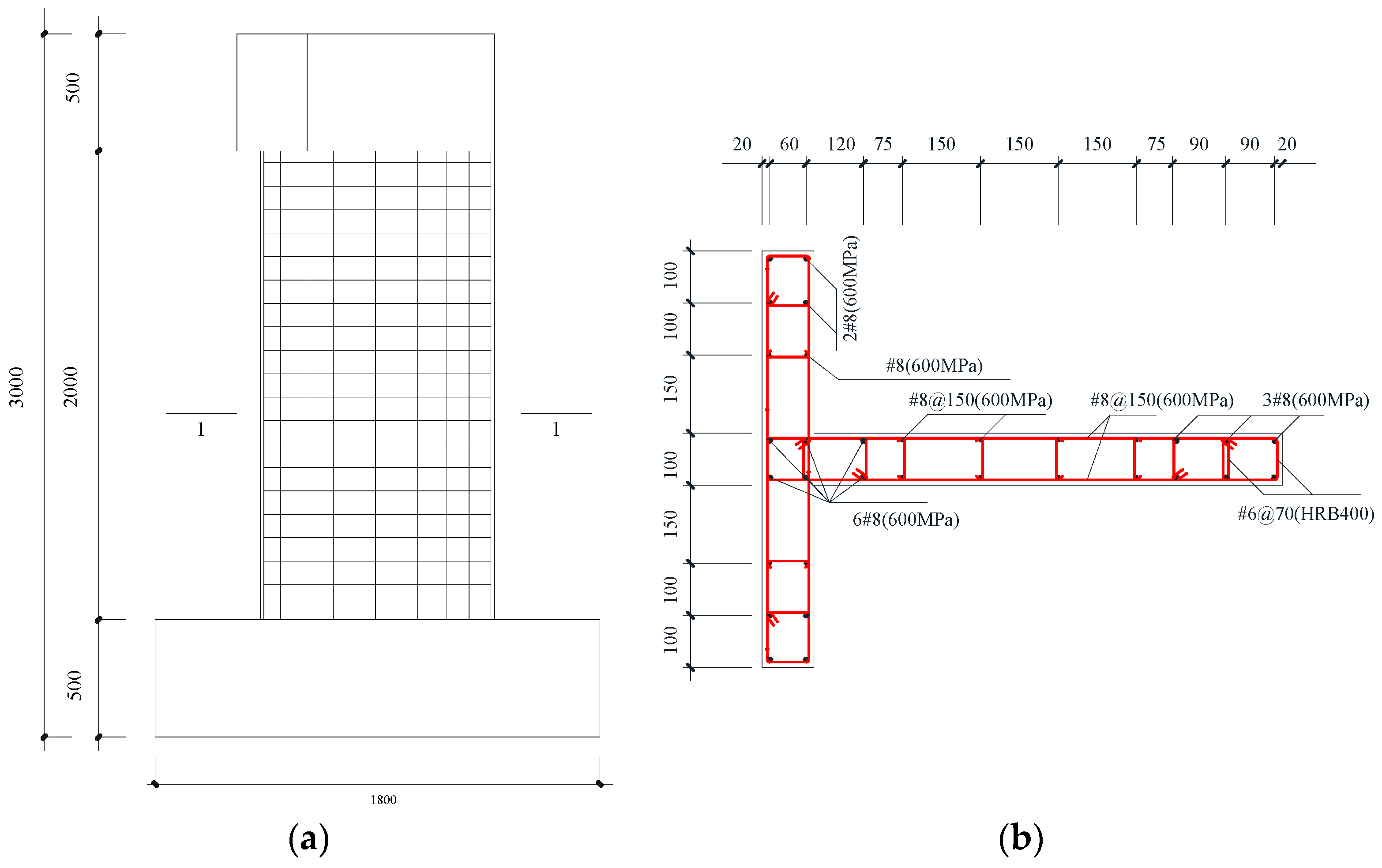
3.1. Details of the Specimen
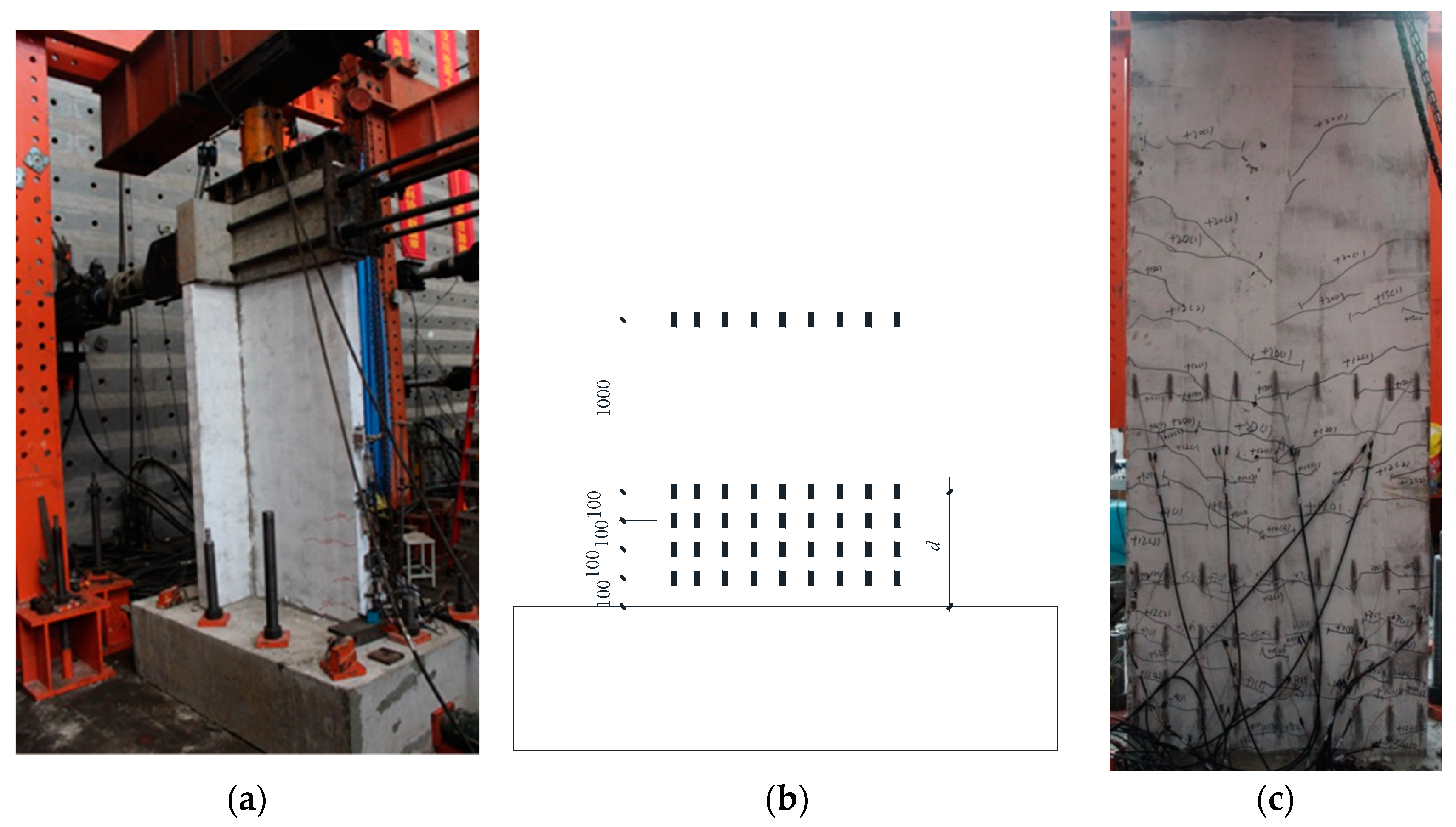
3.2. Loading Setup and Instrumentations
4. Numerical Model
5. Experimental and Numerical Validation for the Proposed Model
6. Parameter Analysis
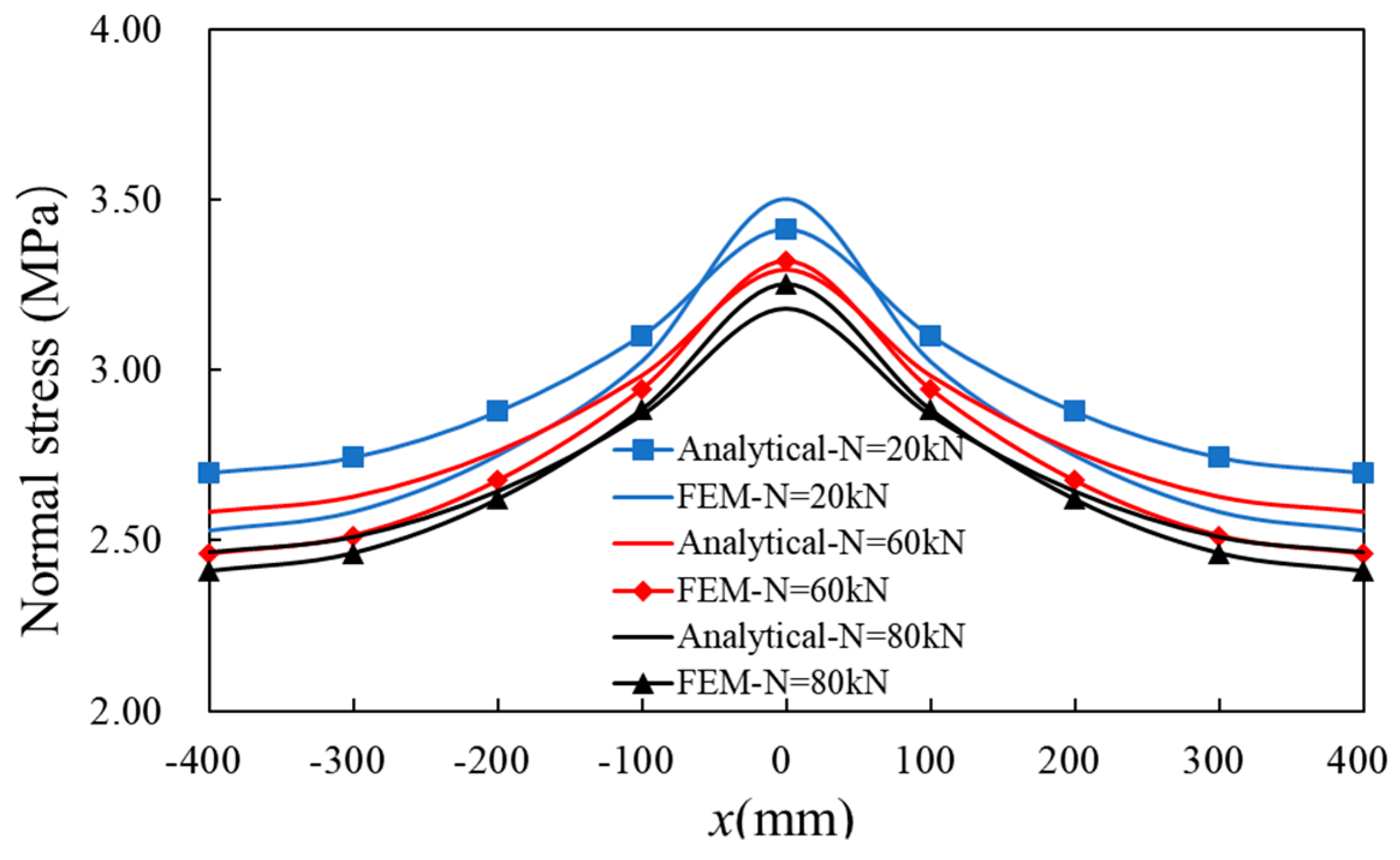
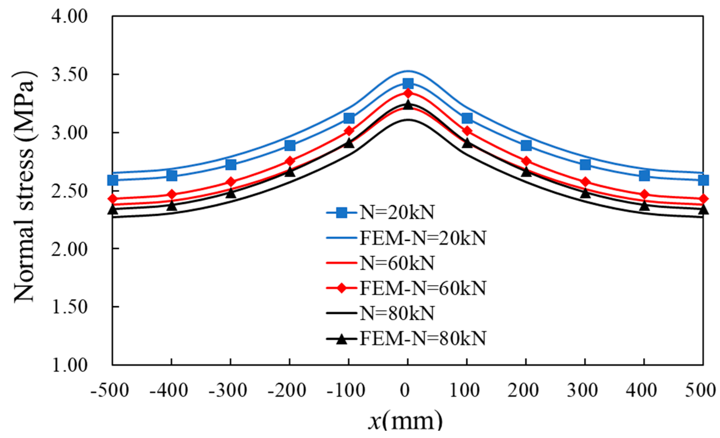
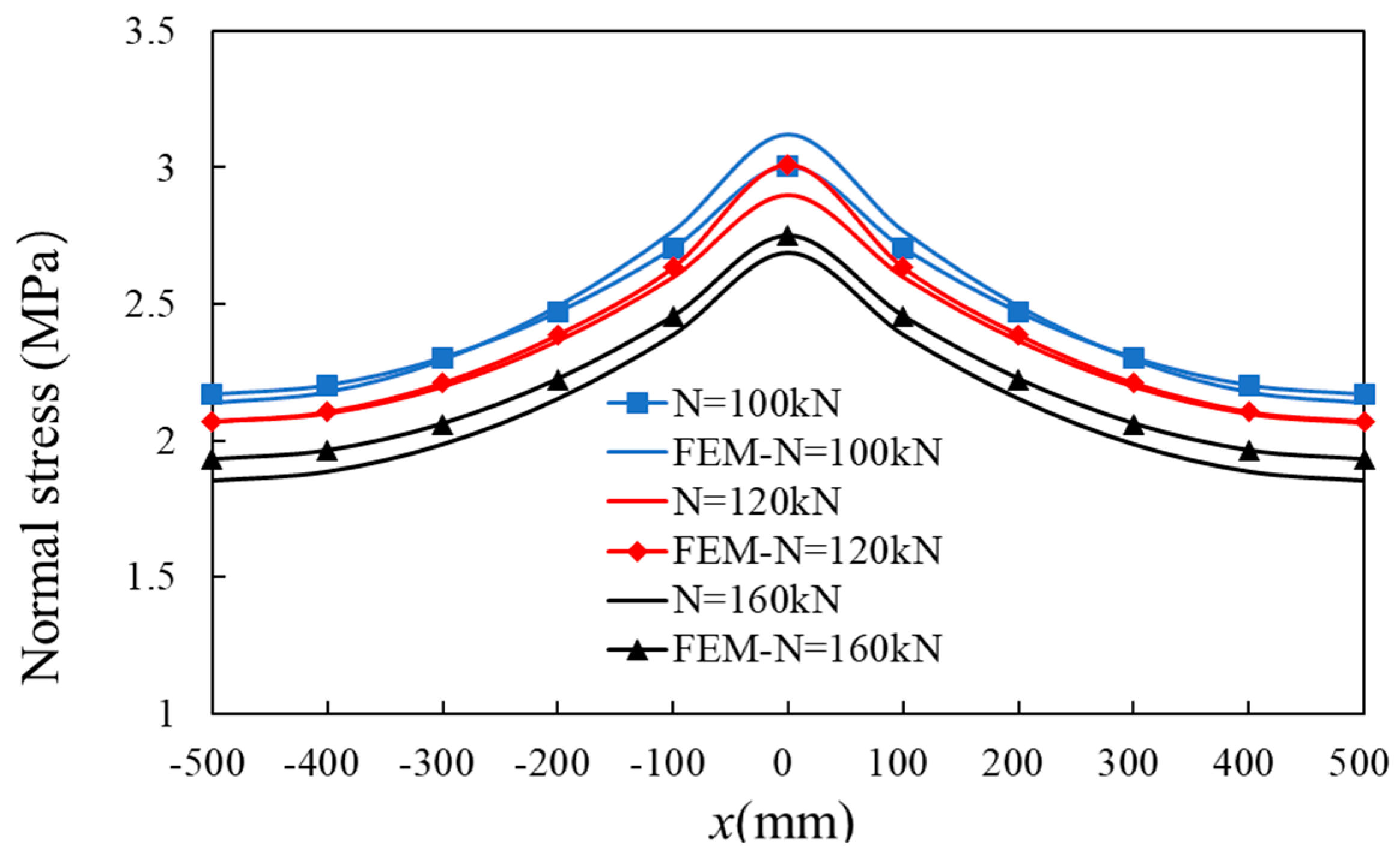
6.1. Axial Load
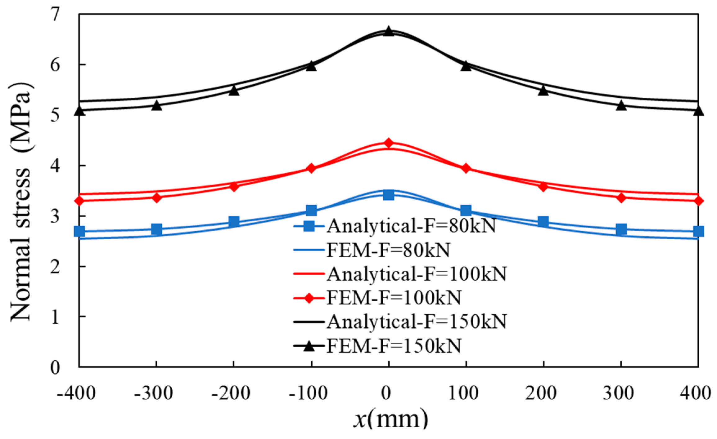
6.2. Lateral Shear Force
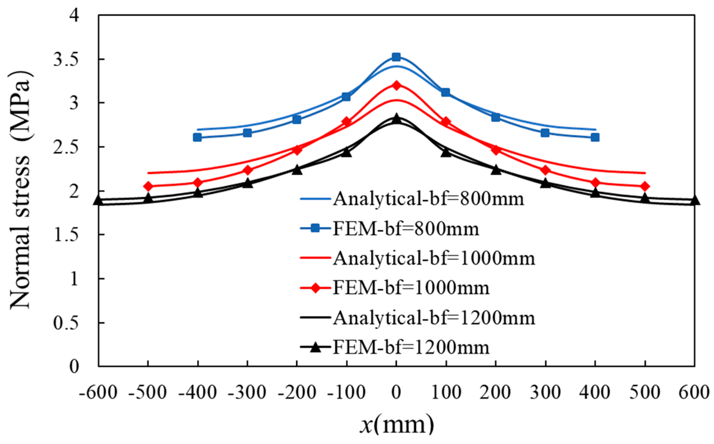
6.3. Flange Length
7. Conclusions
- (1)
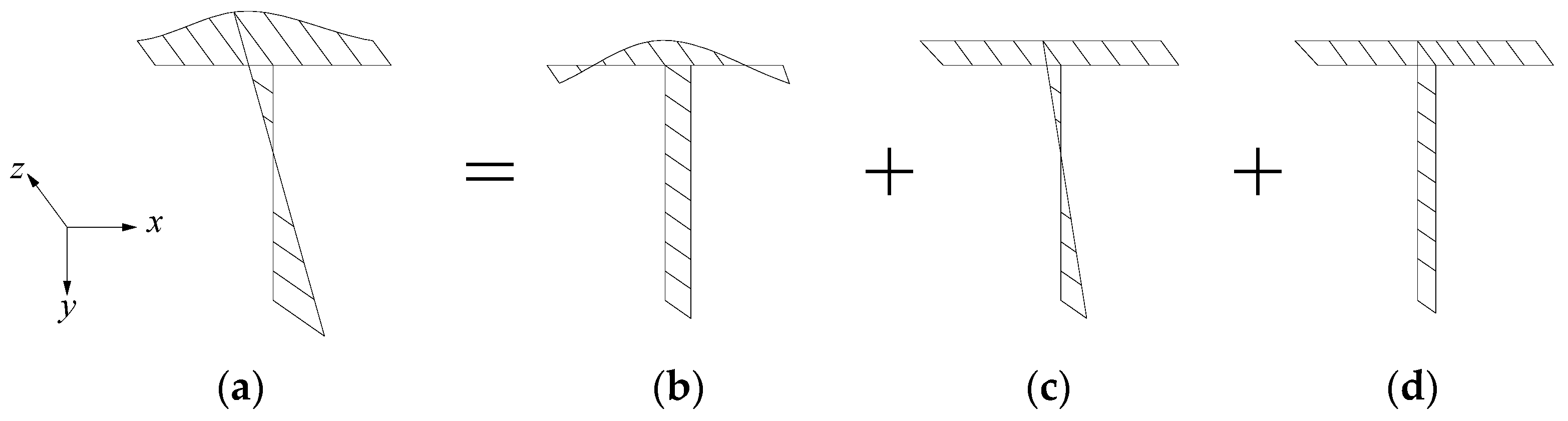
- It is considered that SL warping, flexure, and axial displacement make up the longitudinal deformation of TSSWs. According to the concept of lowest potential energy, the SL warping deformation function is considered to be a quadratic parabola, and the formulae for normal stress and deflection are based on this assumption.
- (2)
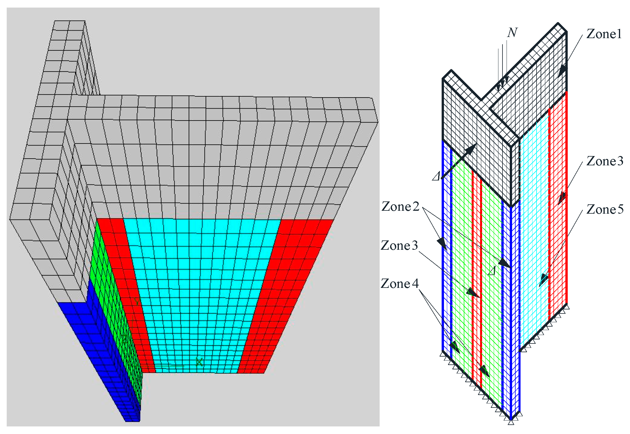
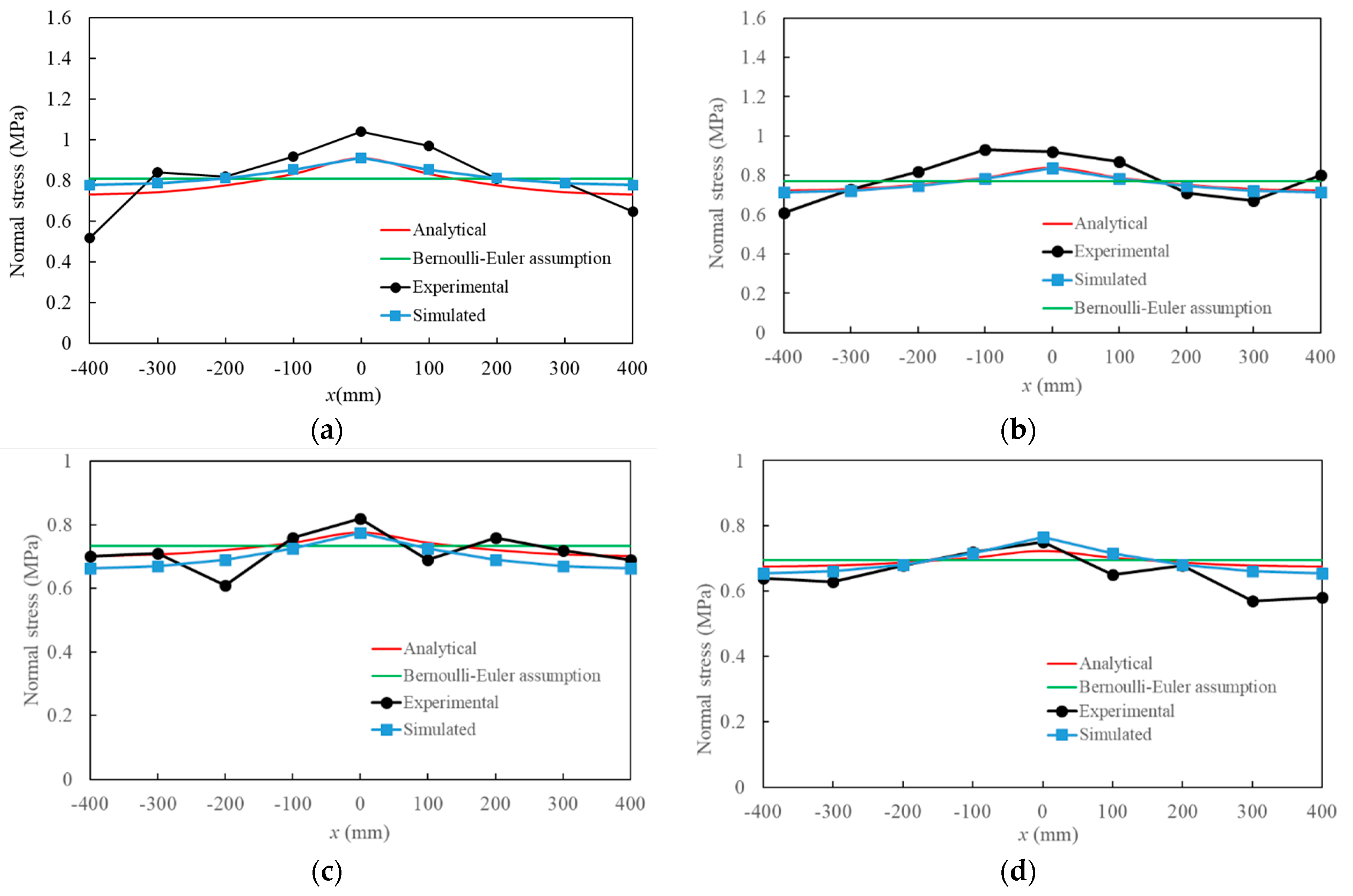
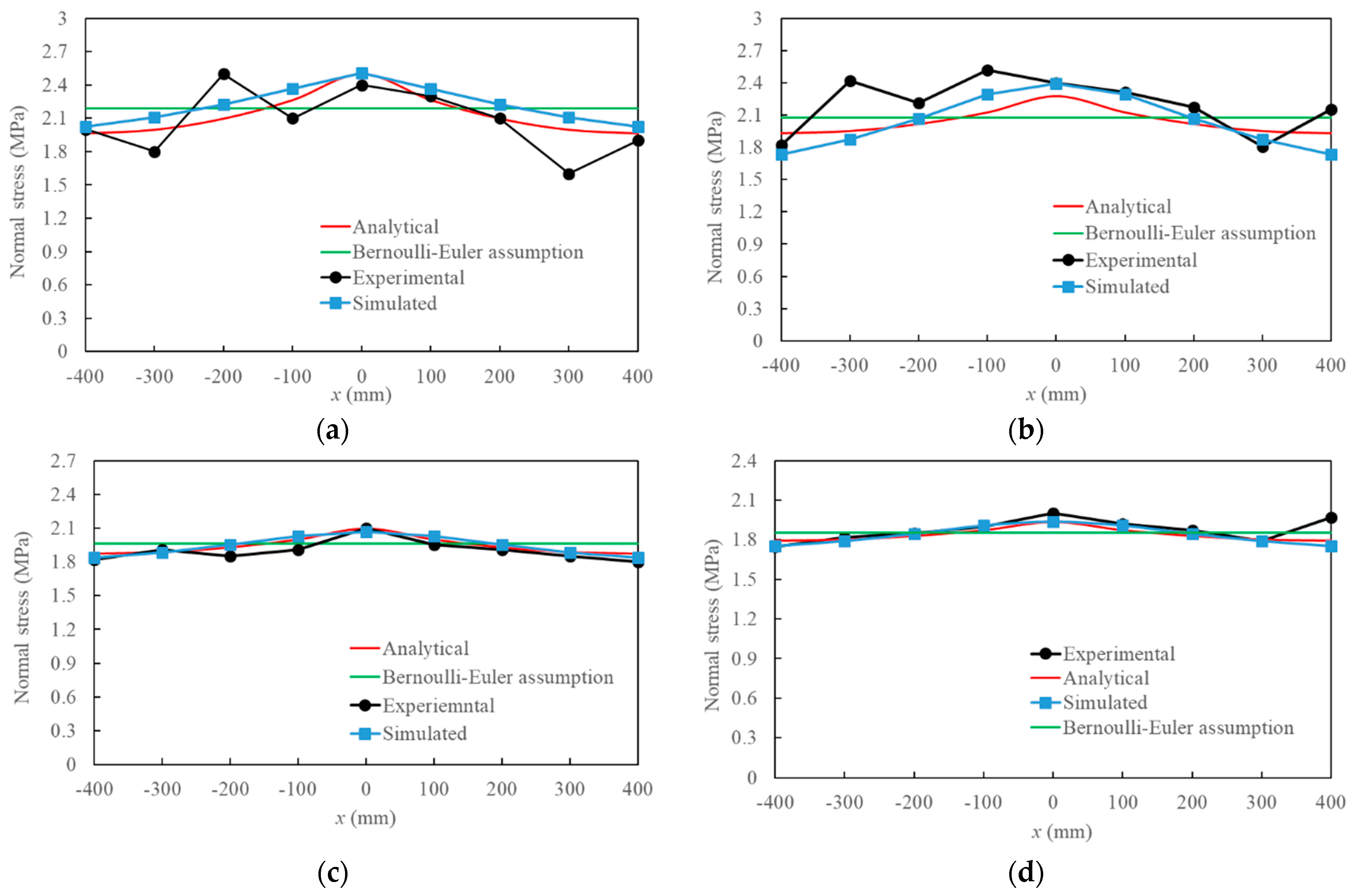
- Three-dimensional FE software VecTor3 is used to create the FE model to examine the shear lag in such walls. Tests are conducted to assess the SL in TSSWs under the combined action of shear force and axial force. The test and simulation findings show that under the influence of a shear force, the flange normal stresses are greater close to the web and less farther away, and a noticeable shear lag phenomena takes place. The Bernoulli–Euler assumption results in an equal distribution of normal stress, which is very different from the experimental, simulated, and analytical normal stress distribution.
- (3)
- The model used in this paper’s analysis produces flange normal stresses that are reasonably consistent with stresses found in simulations and experiments. The comparison indicates that the quadratic parabola assumption of the SL warp displacement of TSSWs is plausible, and the suggested model can accurately estimate the flange normal stresses of the tested and simulated TSSW specimens under axial and shear force.
- (4)
- Based on the verified numerical models of TSSWs, parameter analysis is conducted, and the analysis shows that the wall specimens with various axial forces (20 vs. 60 vs. 80, vs. 100 vs. 120 vs. 160 kN) have a similar SL coefficient, which indicts axial force in these ranges has limited influence on the SL coefficient. The T-shaped wall specimens under larger shear force (80 vs. 100 vs. 150 kN) have the larger SL coefficients, which indicates a more obvious SL effect. A more obvious SL effect occurs in the TSSW specimens with longer flanges (800 mm vs. 1000 mm vs. 1200 mm).
Author Contributions
Funding
Data Availability Statement
Conflicts of Interest
References
- Shan, Z.; Chen, L.; Liang, K.; Su, R.K.L.; Xu, Z. Strengthening Design of RC Columns with Direct Fastening Steel Jackets. Appl. Sci. 2021, 11, 3649. [Google Scholar] [CrossRef]
- Lu, X.; Yang, J.; Jiang, H. Experimental study on seismic behavior of SRC T-shaped shear wall. J. Build. Struct. 2014, 35, 46–52. [Google Scholar]
- Liang, K.; Chen, L.; Su, R.K.L. Seismic behavior of BFRP bar reinforced shear walls strengthened with ultra-high-performance concrete boundary elements. Eng. Struct. 2024, 304, 117697. [Google Scholar] [CrossRef]
- Song, Q.G.; Scordelis, A.C. Shear lag Analysis of T-, I-, and Box Beams. J. Struct. Eng. ASCE 1990, 116, 1290–1305. [Google Scholar] [CrossRef]
- Luo, Q.; Yu, J. Problems of transverse cracking in flange slabs of reinforced concrete continuous box girder bridges. Bridge Constr. 1997, 117, 43–47. [Google Scholar]
- Pantazopoulou, S.J.; Moehle, J.P. Identification of effect of slabs on flexural behavior of beams. J. Eng. Mech. 1990, 116, 91–106. [Google Scholar] [CrossRef]
- Zhang, Z.; Li, B. Seismic performance assessment of slender T-shaped reinforced concrete walls. J. Earthq. Eng. 2016, 20, 1342–1369. [Google Scholar] [CrossRef]
- Wu, Y.; Luo, Q.; Yue, Z. Energy-variational method of the shear lag effect in thin walled box girder. Eng. Mech. 2003, 20, 161–165+160. [Google Scholar]
- Wu, Y.; Lai, Y.; Zhu, Y.; Liu, S.; Zhang, X. Finite element method considering shear lag effect for curved box beams. Eng. Mech. 2002, 19, 85–89. [Google Scholar]
- Zhang, Y.; Zhang, Q.; Li, Q. A variational approach to the analysis of shear lag effect of thin-walled beams with wide flange. Eng. Mech. 2006, 23, 52–56. [Google Scholar]
- Zhang, Y.; Lin, L. A method considering shear lag effect for flexural-torsional analysis of skewly supported continuous box girder. Eng. Mech. 2012, 29, 94–100. [Google Scholar]
- Zhang, Y.H.; Lin, L.X. Shear lag analysis of thin-walled box girders based on a new generalized displacement. Eng. Struct. 2014, 61, 73–83. [Google Scholar] [CrossRef]
- Zhang, Z.; Li, B. Effective stiffness of non-rectangular reinforced concrete structural walls. J. Earthq. Eng. 2016, 22, 382–403. [Google Scholar] [CrossRef]
- Smyrou, E.; Sullivan, T.; Priestley, N.; Calvi, M. Sectional response of T-shaped RC walls. Bull. Earthq. Eng. 2013, 11, 999–1019. [Google Scholar] [CrossRef]
- Zhang, S.; Li, Q.; Guo, Z.; Zhang, J. The shear lag effect and influence of T cross section shear wall with flange. Ind. Constr. 2007, 10, 38–41. [Google Scholar]
- Li, Q.; Zhang, P.; Li, X. Shear lag effect analysis of short-leg shear wall. Ind. Build. 2011, 41, 59–62. [Google Scholar]
- Shi, Q.; Wand, B.; Zheng, X.; Tian, J. Shear lag effect analysis and effective flange width study of the T-shaped shear wall with flange. Build. Struct. 2014, 44, 67–71+40. [Google Scholar]
- Ni, X.; Cao, S. Shear lag analysis of I-shaped structural members. Struct. Des. Tall Spec. Build. 2018, 27, e1471. [Google Scholar] [CrossRef]
- Ni, X.; Cao, S.; Liu, C. Shear lag and effective flange width of T-shaped short-leg shear walls. J. Eng. Res. 2018, 6, 31–52. [Google Scholar]
- Reissner, E. Analysis of shear lag in box beams by the principle of the minimum potential energy. Q. Appl. Math. 1946, 4, 268–278. [Google Scholar] [CrossRef]
- Taherian, A.R.; Evans, H.R. The bar simulation method for the calculation of shear lag in multi-cell and continuous box girder. Proc. Inst. Civ. Eng. Part 2 1977, 63, 881–897. [Google Scholar] [CrossRef]
- Zhang, Z.; Li, B. Effects of the shear lag on longitudinal strain and flexural stiffness of flanged RC structural walls. Eng. Struct. 2018, 156, 130–144. [Google Scholar] [CrossRef]
- Ke, X.J.; Qin, Y.; Chen, S.J.; Li, N. Seismic performance and shear lag effect of T-shaped steel plate reinforced concrete composite shear wall. Eng. Struct. 2023, 289, 116303. [Google Scholar] [CrossRef]
- Hoult, R.D. Shear Lag Effects in Reinforced Concrete C-Shaped Walls. J. Struct. Eng. 2019, 145, 04018270. [Google Scholar] [CrossRef]
- Zhou, S.J. Finite beam element considering shear-lag effect in box girder. J. Eng. Mech. 2010, 136, 1115–1122. [Google Scholar] [CrossRef]
- Li, S.; Hong, Y.; Gou, H.; Pu, Q. An improved method for analyzing shear-lag in thin-walled girders with rectangular ribs. J. Constr. Steel Res. 2021, 177, 106427. [Google Scholar] [CrossRef]
- JGJ3-2010; Technical Specification for Concrete Structures of Tall Building. China Construction Press: Beijing, China, 2010.
- GB/T 50081-2002; Standard for Test Method of Mechanical Properties on Ordinary Concrete. China Architecture & Building Press: Beijing, China, 2003.
- Jafari, A.; Beheshti, M.; Shahmansouri, A.A.; Bengar, H.A. Cyclic response and damage status of coupled and hybrid-coupled shear walls. Structures 2024, 61, 106010. [Google Scholar] [CrossRef]
- ElMohandes, F.; Vecchio, F. Vector3 and Formworks Plususer Manual. 2013. Available online: http://www.civ.utoronto.ca/vector/user_manuals/manual6.pdf (accessed on 25 September 2017).
- Cortés-Puentes, W.L.; Palermo, D. Modeling of RC shear walls retrofitted with steel plates or FRP sheets. J. Struct. Eng. 2011, 138, 602–612. [Google Scholar] [CrossRef]
- Cortés-Puentes, W.L.; Palermo, D. Modelling seismically repaired and retrofitted reinforced concrete shear walls. Comput. Concr. 2011, 8, 541–561. [Google Scholar] [CrossRef]
- Cortés-Puentes, W.L.; Palermo, D. Modeling of Concrete Shear Walls Retrofitted with SMA Tension Braces. J. Earthq. Eng. 2020, 24, 555–578. [Google Scholar] [CrossRef]
- Palermo, D.; Vecchio, F.J. Behavior of Three-Dimensional Reinforced Concrete Shear Walls. Struct. J. 2002, 99, 81–89. [Google Scholar]
- Palermo, D.; Abdulridha, A.; Charette, M. Flange participation for seismic design of reinforced concrete shear walls. In Proceedings of the 9th Canadian Conference on Earthquake Engineering, Ottawa, ON, Canada, 26–29 June 2007. [Google Scholar]
- Ni, X.; Cao, S.; Aoude, H. Seismic performance of concrete walls reinforced by high-strength bars: Cyclic loading test and numerical simulation. Can. J. Civ. Eng. 2021, 48, 1481–1495. [Google Scholar] [CrossRef]
- Vecchio, F. Disturbed stress field model for reinforced concrete: Formulation. J. Struct. Eng. 2010, 126, 1070–1077. [Google Scholar] [CrossRef]
- Hognestad, E. Study of Combined Bending and Axial Load in Reinforced Concrete Members; University of Illinois at Urbana Champaign: Champaign, IL, USA, 1951. [Google Scholar]
- Vecchio, F.J.; Collins, M.P. Compression response of cracked reinforced concrete. J. Struct. Eng. ASCE 1993, 119, 3590–3610. [Google Scholar] [CrossRef]
- Kupfer, H.; Hilsdorf, H.K.; Rusch, H. Behavior of concrete under biaxial stresses. J. Proc. 1969, 66, 656–666. [Google Scholar] [CrossRef] [PubMed]
- Vecchio, F.J.; Lai, D. Crack shear-slip in reinforced concrete elements. J. Adv. Concrete Technol. 2004, 2, 289–300. [Google Scholar] [CrossRef]


| Constitutive Behavior | Model |
|---|---|
| Compression pre-peak | Parabola [38] |
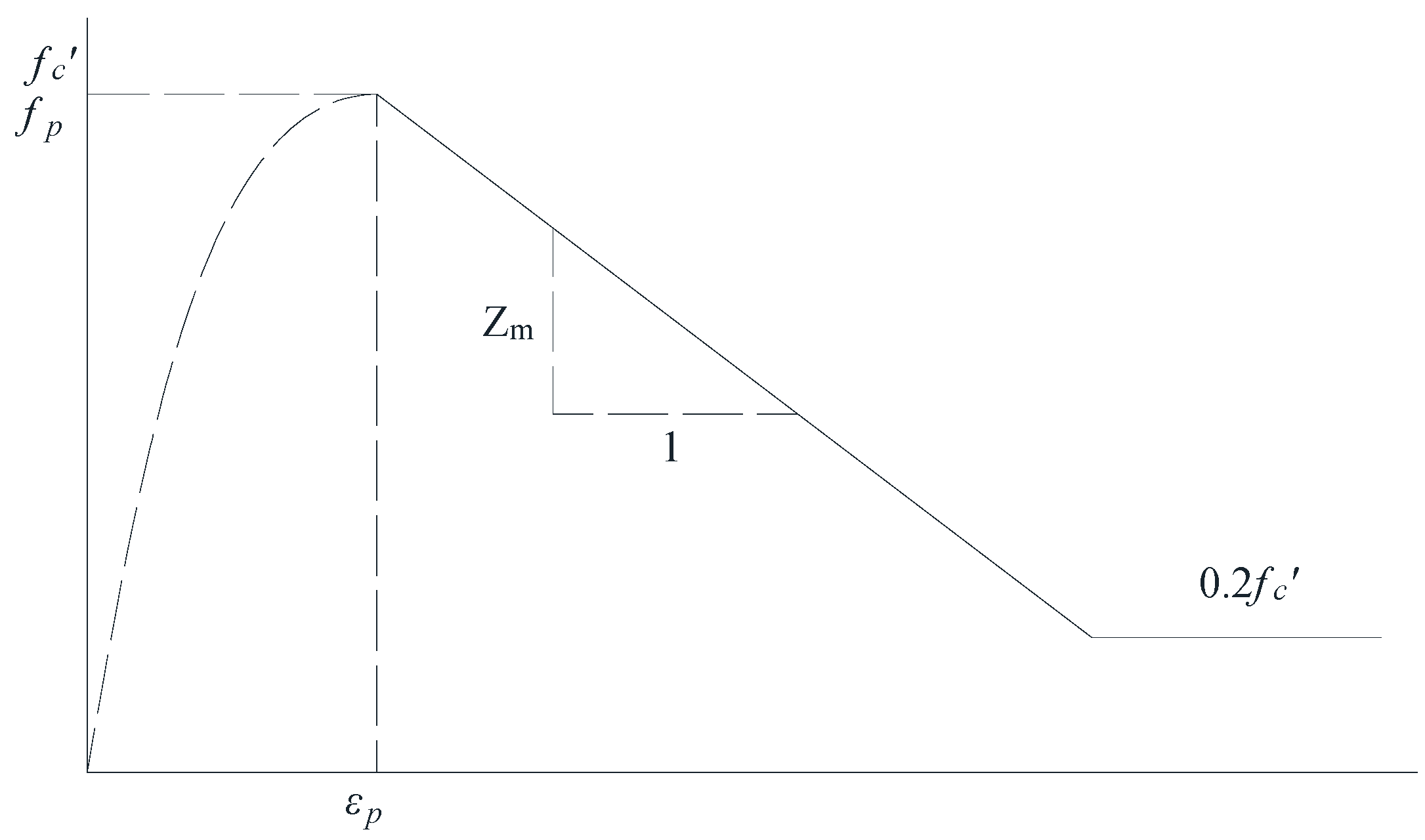
| Compression post-peak | Modified Kent and Park [37] |
| Compression softening | Vecchio 1993-A [e1/e2-Form] [39] |
| Tension stiffening | Modified Bentz Model [36] |
| Tension softening | Linear |
| Confined strength | Kupfer/Richart [40] |
| Dilation | Variable-Kupfer |
| Cracking criterion | Mohr–Coulomb [Stress] |
| Crack stress calc | Basic [DSFM/MCFT] |
| Crack width | Check Aggregate 2.5 mm max crack width [Default] |
| Crack slip calc | Vecchio and Lai [41] |
| N (kN) | σ | λ | |||
|---|---|---|---|---|---|
| Analytical | Simulated | Analytical | Simulated | ||
| Flange length = 800 mm, F = 80 kN | |||||
| 20 | 3.00 | 3.41 | 3.50 | 1.14 | 1.17 |
| 60 | 2.88 | 3.30 | 3.32 | 1.14 | 1.15 |
| 80 | 2.76 | 3.18 | 3.25 | 1.15 | 1.18 |
| 100 | 2.65 | 3.06 | 3.20 | 1.15 | 1.21 |
| 120 | 2.53 | 2.94 | 3.02 | 1.16 | 1.19 |
| 160 | 2.29 | 2.71 | 2.75 | 1.18 | 1.20 |
| Flange length = 1000 mm, F = 80 kN | |||||
| 20 | 2.90 | 3.42 | 3.53 | 1.18 | 1.22 |
| 60 | 2.69 | 3.21 | 3.34 | 1.19 | 1.24 |
| 80 | 2.59 | 3.11 | 3.24 | 1.20 | 1.25 |
| 100 | 2.48 | 3.00 | 3.12 | 1.21 | 1.26 |
| 120 | 2.38 | 2.90 | 3.01 | 1.22 | 1.27 |
| 160 | 2.16 | 2.69 | 2.75 | 1.24 | 1.27 |
| F (kN) | σ | λ | |||
|---|---|---|---|---|---|
| Analytical | Simulated | Analytical | Simulated | ||
| 80 | 3.00 | 3.41 | 3.50 | 1.14 | 1.17 |
| 100 | 3.61 | 4.33 | 4.45 | 1.20 | 1.23 |
| 150 | 4.98 | 6.61 | 6.67 | 1.33 | 1.34 |
| bf (mm) | σ | λ | |||
|---|---|---|---|---|---|
| Analytical | Simulated | Analytical | Simulated | ||
| 800 | 3.00 | 3.41 | 3.50 | 1.14 | 1.17 |
| 1000 | 2.53 | 3.03 | 3.20 | 1.20 | 1.26 |
| 1200 | 2.20 | 2.77 | 2.83 | 1.26 | 1.29 |
Disclaimer/Publisher’s Note: The statements, opinions and data contained in all publications are solely those of the individual author(s) and contributor(s) and not of MDPI and/or the editor(s). MDPI and/or the editor(s) disclaim responsibility for any injury to people or property resulting from any ideas, methods, instructions or products referred to in the content. |
© 2024 by the authors. Licensee MDPI, Basel, Switzerland. This article is an open access article distributed under the terms and conditions of the Creative Commons Attribution (CC BY) license (https://creativecommons.org/licenses/by/4.0/).
Share and Cite
Liu, J.; Hou, Y.; Wang, H.; Ni, X. Experimental and Analytical Study on Shear Lag Effect of T-Shaped Reinforced Concrete Shear Walls. Buildings 2024, 14, 1875. https://doi.org/10.3390/buildings14061875
Liu J, Hou Y, Wang H, Ni X. Experimental and Analytical Study on Shear Lag Effect of T-Shaped Reinforced Concrete Shear Walls. Buildings. 2024; 14(6):1875. https://doi.org/10.3390/buildings14061875
Chicago/Turabian StyleLiu, Jianzhao, Yonghui Hou, Hongyan Wang, and Xiangyong Ni. 2024. "Experimental and Analytical Study on Shear Lag Effect of T-Shaped Reinforced Concrete Shear Walls" Buildings 14, no. 6: 1875. https://doi.org/10.3390/buildings14061875