Numerical Modeling of Four-Pile Caps Using the Concrete Damaged Plasticity Model

Abstract

Four-pile caps made from concrete are essential elements for the force transfer from the superstructure to piles or pipes. Due to the difficulties in carrying out full-scale tests and all the instrumentation involved, the use of numerical models as a way to study the mechanical behavior of these elements presents itself as a good alternative. Such numerical studies usually provide useful information for the update and improvement of normative standards and codes. The concrete damaged plasticity (CDP) constitutive model, which combines damage and plasticity with smeared-crack propagation, stands out in the simulation of reinforced concrete. This model is composed of five parameters: dilatation angle (ψ), eccentricity (ϵ), ratio between biaxial and uniaxial compressive strength (σ_bo/σ_co), failure surface in the deviator plane normal to the hydrostatic axis (K_c), and viscosity (μ). For unidimensional elements, the values of the CDP parameters are well defined, but for volumetric elements, such as concrete pile caps, there is a gap in the literature regarding the definition of these values. This fact ends up limiting the use of the CDP on these structural elements due to the uncertainties involved. Therefore, the aim of this research was to calibrate two numerical models of concrete four-pile caps with different failure modes for the evaluation of the sensitivity of the CDP parameters, except for ϵ, which remained constant. As a result, the parameters σ_bo/σ_co and K_c did not significantly influence the calibration of the force × displacement curves of the simulated structures. Values of ψ and μ equal to 36° and 1 × 10⁻⁴, respectively, are recommended for “static” analysis, while for “quasi-static” analysis, ψ values ranging between 45° and 50° are suggested according to the failure mode. The results also showed to be sensitive to the constitutive relation of concrete tensile behavior in both modes of analysis. For geometric parameterization, the “static” analysis is recommended due to the lower coefficient of variation (3.29%) compared to the “quasi-static” analysis (19.18%). This conclusion is supported by the evaluation of the ultimate load of the numerical models from the geometrically parametric study compared to the results estimated by an analytical model.

1. Introduction

Pile caps are structural elements that transfer loads from superstructures to piles. Some limitations are identified in experimental campaigns that studied concrete four-pile caps. Rupture force, for example, is limited to 2500 kN in approximately 95% of literature works. As a result, few records are available from a single experimental campaign [1]. Another limiting factor refers to the geometry of the column, which is mostly restricted to square sections. Despite these limitations, these studies are extremely important for the technical community, especially in order to corroborate relevant information for the design and updating of regulatory codes.

The Brazilian standard ABNT NBR 6118 [2] allows the use of non-linear numerical models to evaluate the performance of reinforced concrete structures. In this way, numeric solvers are complementary tools, which enable deeper investigation of structure behavior.

Due to the difficulty of measurements in physical models, the use of numerical models for the simulation of mechanical behavior of pile caps is justified since these models help to understand the behavior of these elements. As pile caps represent discontinuity regions (D-regions), the boundary conditions significantly influence the behavior of the stress flow. The analysis of test results (physical models) from the technical literature [1,3,4,5,6] reveals a lack of standardization in the support and loading elements, which makes the right discretization of numerical models a hard task. These conditions can influence the estimate of the ultimate force in numerical modeling by up to 100% [7].

For this reason, it is essential to understand the software functionalities and its input parameters for simulations. Numerical models were utilized to replicate the behavior of experimental pile cap [8,9], leading to a satisfactory calibration. Consequently, this methodology was adopted to simulate the mechanical behavior of pile caps with two, three, four, and six piles [10,11,12,13,14].

Although numerical models for pile caps have produced satisfactory results, some studies described some trouble in replicating experimental tests [15,16]. For a better understanding of boundary condition influence on numerical results, Luchesi et al. [17] conducted an analysis. However, it should be noted that these findings are limited to models of two-pile caps.

Melendez et al. [18] proposed a simplification in the modeling of volumetric elements (D-regions), applying this methodology for four-pile caps. This simplification disregards the tensile strength of concrete and allows the identification of compressive stress flows for the idealization of complex models of struts and ties. However, the simulation results are conservative for the estimation of the ultimate capacity of these elements.

A model that stands out for simulating reinforced concrete and its distributed smeared-crack propagation is the CDP (concrete damaged plasticity) model. This model combines damage and plasticity for the simulation of material behavior and can accurately predict the non-linear behavior of concrete. Its formulation considers a triaxial stress state, which makes it suitable for the simulation of elements’ mechanical behavior like beams, shear walls, and slabs. In the case of two-pile caps, the CDP model can precisely reproduce the experimental force × displacement curve [19]. However, two-pile caps present a behavior with bidirectional flow of stress, while four-pile caps are characterized by a tridimensional stress distribution.

For the adoption of the concrete damaged plasticity (CDP) model (more details about the CDP parameters can be seen in Appendix A), it is necessary to insert the uniaxial stress × strain curves for compression and tension of the concrete. It also requires the inclusion of the following parameters: dilatation angle ($\psi$), eccentricity ($ϵ$), biaxial and uniaxial compressive strength ratio (${\sigma }_{bo}/{\sigma }_{co}$), failure surface in the deviator plane normal to the hydrostatic axis ($K_c$), and viscosity ($\mu$). Considering three-dimensional solids, the absence of simplifying assumptions can be noticed, such as for pile caps (lack of information about the CDP parameters). As a reference, for one-dimensional reinforced concrete structural elements (beams or columns), in which the CDP parameters are very well established, ψ values are established in the range of 30° to 40° [20,21,22].

Although the CDP model is a viable option for analyzing the behavior of structures, scientific research has investigated solutions for the calibration of its parameters due to the lack of agreement in the definition of these values [23,24]. Furthermore, this model is not commonly utilized for four-pile caps, as it can be checked in

Table 1. CDP parameter values according to strucutral elements.

References	Structural Element	Analysis	$\mathit{\psi }$ (°)	$\mathit{ϵ}$	${\mathit{\sigma }}_{\mathit{b}\mathbf{0}}\mathbf{/}{\mathit{\sigma }}_{\mathit{c}\mathbf{0}}$	${\mathit{K}}_{\mathit{c}}$	$\mathit{\mu }$
[25]	Standard values	-	36	0.1	1.16	0.667	-
Ali, Kim, and Cho [26]	Shear wall	NE	30	-	-	-	-
Dawood, Elgawady, and Hewes [27]	Precast post-tensioned bridge piers	Static	1	0.1	1.16	0.66	0
Dong et al. [28]	Shear walls	Static	30	0.1	1.16	0.6667	0.0001
Genikomsou and Polak [29]	Slab	Quasi-static	40	0.1	1.16	0.667	0.00001
Milligan, Polak, and Zurell [30]	Slab	Static/ quasi-static *	45	0.1	1.16	0.667	-
Husain, Eisa, and Hegazy [31]	Shear walls	Quasi-static	37	0.1	1.16	0.67	0.001
Jha, Roshan, and Bishnoi [32]	Specimen CAMUS: a 1/3-scale model of a representative 5-story reinforced concrete building	NE	55	1.25	1.16	0.667	0.0005
Kaushik and Dasgupta [33]	Slab structural wall junction of RC building	Static	55	0.1	1.16	0.667	0.01
Li, Hao, and Bi [34]	Columns	Static	30	0.1	1.16	0.666	0.0001
Liu et al. [35]	Concrete-filled steel tubular column for steel beam connections	NE	30	0.1	1.16	0.667	0.005
Michal and Andrzej [36]	“d” regions of RC structures	Static	15	-	-	-	0.0001
Najafgholipour et al. [37]	Beam–column connections	Static	35	0.1	1.16	0.7	-
Pavlović [38]	Shear connectors	Quasi-static	36	0.1	1.16	-	-
Pelletier and Léger [39]	Reinforced concrete cores	NE	13	90	1.16	0.667	-
Ren et al. [40]	Prestressed precast concrete Bridge deck panels	Static	38	0.1	1.76	0.667	0.0005
Surumi, Jaya, and Greeshma [41]	Shear walls	NE	38	0.1	1.16	0.67	0
Vojdan and Aghayari [42]	Shear walls	NE	36/40	0.1	1.16	0.667	-
Wang et al. [43]	Concrete-infilled double steel corrugated-plate walls	NE	30	0.1	1.16	0.6667	-
Wei, Richard Liew, and Fu [44]	Novel partially connected buckling-restrained steel plate shear walls	Quasi-static	36	0.1	1.16	-	-
Szczecina and Winnicki [45]	Frame corner	Static	5	0.1	1.16	0.667	0.0001
Cuong-Le, Minh, and Sang-To [46]	Beams/slab	NE	30/40	0.1	1.16	0.7	-
Alfarah, López-Almansa, and Oller [47]	Frame	NE	13	0.1	1.16	0.7
Bash et al. [19]	Two-pile cap	NE	26	0.1	1.16	0.667	0
Silva, Christoforo, and Carvalho [23]	Shear walls	Static	46.4	0.1	1.16	0.58	0.00001
Neuberger et al. [48]	Corbels	Static	48	0.1	1.16	0.667	0.0005
Reginato et al. [49]	Corbels	Static	42	0.1	1.16	0.667	0.0001
Azevedo Palhares et al. [50]	Slab	Static	25	0.1	1.16	0.667	0.0001
Arthi and Jaya [51]	Precast shear wall–slab connection	NE	38	0.1	1.12	0.67	0.666
Hu, Fang, and Benmokrane [52]	UHPC shear walls reinforced	NE	54	0.1	1.07	0.666	-
Scamardo et al. [53]	Masonry	Static	10	0.1	1.16	0.667	0.002
Nguyen, Tan, and Kanda [54]	Precast prestressed concrete hollow core	Quasi-static	28 **	0.1	1.16	0.667
Madkour, Maher, and Ali [55]	Slab	Static	40	0.1	1.16	0.667	0.00001

* Structural analysis can be performed after calibration with Standard and Explicit solvers. ** Authors suggest a model calibration study for the definition of parameter values.

. However, this table presents a considerable range of information about CDP parameters for D-region analysis. It is also important to highlight that studies embraced in Table 1 are a result of a wide (without limiting by the research’s year of publication) literature review. The main objective of this literature review was to have the variation of CDP parameters covered for two-dimensional structural elements. For such purpose, the combined keywords were “CDP”; “Concrete Damage Plasticity”; “Pile Caps”; “Slab”; “Shear”; “Wall”; “Masonry”; and “Corbels”. It is noteworthy that in this search, the use of the CDP model for concrete four-pile caps was not identified, which motivated this research.

The angle of dilatation ($\psi$) influences the material’s ductility and depends on the plastic deformation and confinement pressure [21]. Regarding viscous plastic regularization ($\mu$), it shows a considerable influence on computational effort. In addition, an improper definition of this last parameter leads to overestimation of concrete tensile strength [45,49]. In this context, and based on the results presented in Table 1, it can be seen that these parameters varied in a significant range for the use of the CDP model. Furthermore, Table 1 indicates different modes or methods of analysis associated with CDP, which are “static” and “quasi-static”.

Najafgholipour and Sarhadi [56] contextualized that for numerical models that present a cumbersome definition of boundary conditions or non-linearity of the material, the “static” analysis can result in convergence problems, and in this case, the use of the related algorithm “quasi-static” mode presents greater efficiency.

Studies for the calibration of CDP focus on the variation of ψ values combined with other parameters [24,48]. Given the significant variation found in values of the CDP parameters (ψ and μ) and the lack of analysis of results for the simulation of the mechanical behavior of concrete four-pile caps, the need for specific studies for these elements is evident. In the same way, the analysis of the impact of these variables with the different analysis modes or methods used (“static” and “quasi-static”) is necessary.

Also, considering the need for a deeper understanding of the behavior of concrete four-pile caps in conditions that go beyond the limits/scope of literature tests, this study adopted different modes of analysis to evaluate the influence of extrapolated geometries (parametric study) of the calibrated models. The objective was to identify the reliability of these approaches for geometry parameterization. The results of this research contribute by specifying the use of CDP for simulations of these elements in situations that have not yet been verified due to the limitations of experimental tests.

With the purpose of achieving the study target, this work was divided into three steps. First, the force × displacement curves were calibrated. For this, the influence of CDP parameters on two four-pile caps with distinct failure modes was analyzed. Subsequently, the calibrated models were double-checked via different solvers. Finally, a parametric numerical study varying the geometrical dimensions was executed to evaluate the predicted failure loads according to Meléndez et al. [57]. Then, the results of the parametric study were also checked in different solvers.

2. Methodology

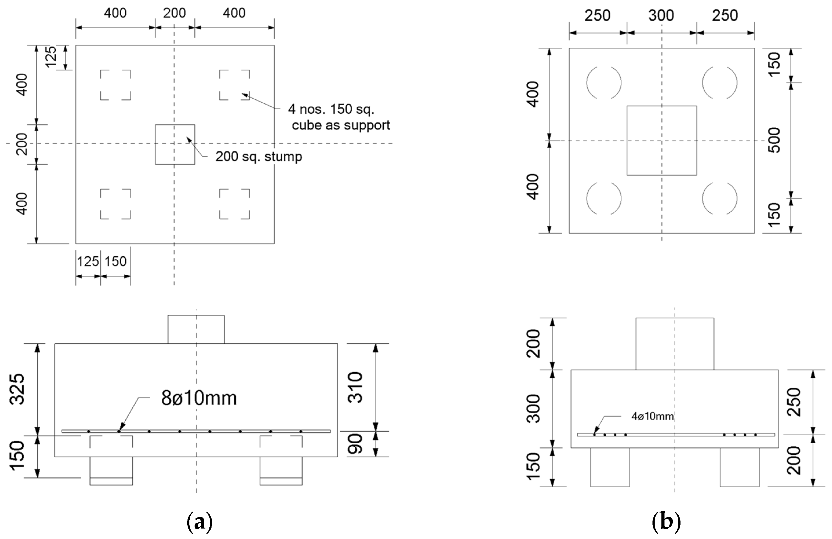
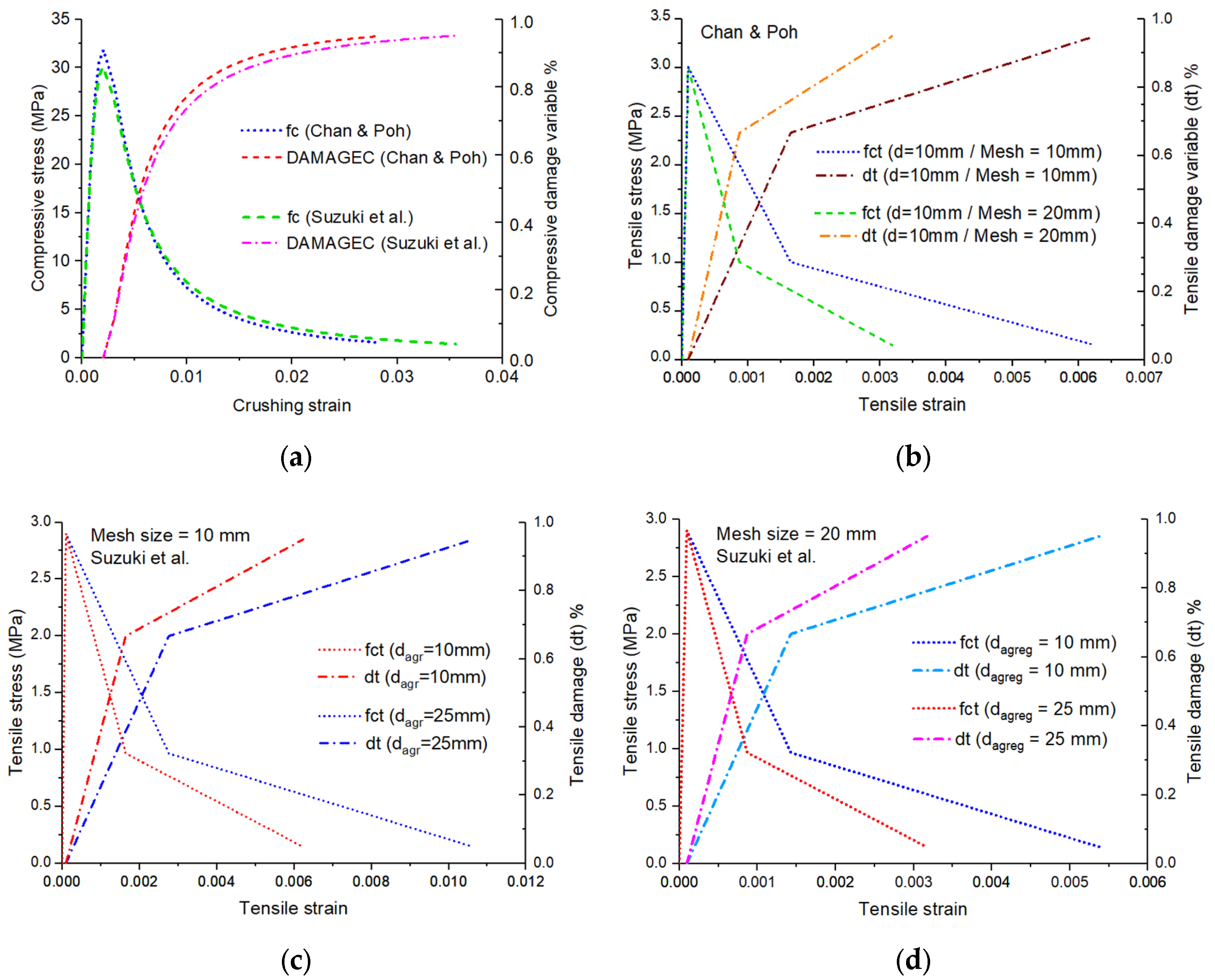
2.1. Experiments and Material Properties

The experimental studies of Chan & Poh [5] and Suzuki, Otsuki, & Tsubata [3] were adopted for the model calibration (Figure 1). It can be noted that two distinct failure modes were then simulated.

Table 2. Material properties.

Model		Concrete				Steel Reinforcement
		Pile Cap			Column and Piles
	${\mathbf{F}}_{\mathbf{e}\mathbf{x}\mathbf{p}}$ (kN)	${\mathbf{f}}_{\mathbf{c}}$ (MPa)	${\mathbf{f}}_{\mathbf{c}\mathbf{t}}$ (MPa)	${\mathbf{E}}_{\mathbf{c}}$ (MPa)	${\mathbf{E}}_{\mathbf{c}}$ (MPa)	${\mathbf{A}}_{\mathbf{s},\mathbf{T}}$ (cm2)	${\mathbf{f}}_{\mathbf{y}}$ (MPa)	${\mathbf{f}}_{\mathbf{u}}$ (MPa)	${\mathbf{E}}_{\mathbf{s}}$ (GPa)
Pile Cap A [5]	1230	31.76	3.00	31,116.22	37,277.87	6.28	480	552	200
BPC 30-30 [3]	1034	30.09	2.90	30,606.90		5.70	405	592	200

shows the material properties adopted for numerical modeling. The Poisson ratios ($\nu$) for concrete and steel were adopted as 0.20 and 0.30, respectively.

The tensile strength ($f_{ct}$) and modulus of elasticity ($E_c$) of the concrete were determined through Equations (1) and (2), respectively, as recommended by Eurocode 2 [58]. The concrete compressive strength ($f_{ck}$) was defined based on experimental results [3,5], while the column and pile were considered to have greater stiffness than the pile cap. The $f_{ck}$ value adopted was equal to the average value of concrete compressive strength from the laboratory tests (column “$f_c$” of Table 2) of the respective experimental campaigns. Regarding material properties, these were estimated according to the methodology found in the literature [48,59,60].

$$f_{ct}=0.3{f_{ck}}^{2/3}$$

(1)

$$E_c=22{\left[f_{ck}/10\right]}^{0.3}$$

(2)

where $f_{ck}$: characteristic concrete compressive strength (MPa), $f_{ct}:$ concrete tensile strength (MPa), and $E_c:$ modulus of elasticity (MPa).

2.2. Analisys Methods

The analysis modes or methods discussed in this work are considered based on two available solvers in ABAQUS^® software (version 6.13) for the simulation of numeric models: ABAQUS^®/Standard, which ensures convergence of results for each increment, and ABAQUS^®/Explicit, which allows a quasi-static procedure [25].

ABAQUS^®/Explicit presents non-linear explicit dynamic formulation for the analysis of structures under dynamic and quasi-static loading. In this context, the material deformation is determined by the difference between increments, which presents a decrease in computational cost. Still, the criteria of low-kinetic-energy values in the system must be monitored so that reliable results can be guaranteed [25]. Models were processed with “double precision” and a displacement of 0.25 mm/s for the calibration of CDP parameters. The criteria of dissipated energy to ensure the quasi-static procedure were assured with a ratio of the whole kinetic energy to internal and external energies of less than 1% for all models processed.

In contrast, ABAQUS^®/Standard is a static solver with viscoplastic regularization (μ) due to computational difficulties faced in the iterative process. In the attempts for model convergence, errors may occur for complex geometries. In addition, a higher computational effort is required when compared to ABAQUS/Explicit.

The average time of simulation according to the value of μ was evaluated for both analysis methods considered in this work. A computer with an Intel I7-11800H processor, 16 Gb RAM, an SSD hard disk with 1 TB capacity, and a NVidia 3060TI discrete graphics card with 6 GB of GDDR6.

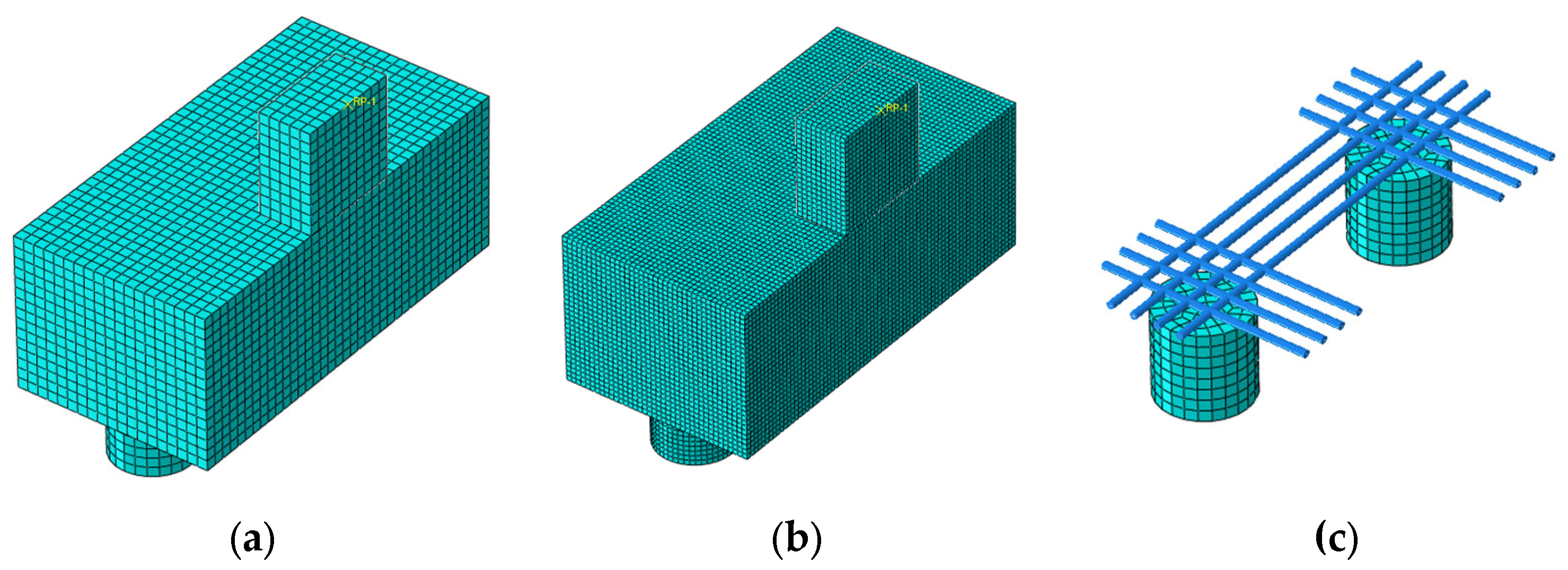
2.3. Numerical Modeling

A C3D8R finite element (8-node linear brick with reduced integration and hourglass control) and a T3D2 element (a 2-node linear 3-D truss) were used to simulate the concrete and steel reinforcement. The T3D2 elements were assumed to be embedded into C3D8R elements (perfect adhesion). The bottom of the column and the upside surface of each support connection were specified with a tie constraint.

When analyzing numerical models for the prediction of slab behavior, it is identified that finite elements without reduced integration better represent the post-peak behavior of the structure. Despite this benefit, these elements present shear lock behavior, which influences the displacement results [50]. Given the problems faced in numerical models related to the reproduction of pile caps’ displacements [15], the present research chose to use the element with the lowest stiffness, that is, without the effects of shear locking. In the literature, it can be observed that the C3D8R element associated with CDP is used in the analysis of two-pile caps [19] and slabs [29].

A uniaxial compression stress–strain relation of concrete, as specified by Carreira and Chu [52], was adopted to fulfill the input parameters of CDP. In the case of the tensile stress–strain relation, due to the mesh sensitivity effects when there is no reinforcement in significant regions of the model [18], a fracture energy model was adopted according to methodologies in the literature [30,61,62].

According to Model Code 1990 [63], fracture energy ($G_F$) is a function of concrete compressive strength ($f_c$) (Equation (3)). $G_{fo}$ was defined through interpolation of the maximum aggregate size ($d_{max}$) by Equation (4) [61]. The proposal of Model Code 2010 [64] resulted in higher strength in the preliminary studies.

$$G_F=G_{fo}{\left(f_c/10\right)}^{0.7}$$

(3)

$$G_{fo}=(0.00005 d_{max}^2-0.0005 d_{max}+0.026)$$

(4)

where $f_c$ is concrete compressive strength (MPa) and $d_{max}$ is the maximum aggregate diameter (mm).

The maximum aggregate diameter ($d_{max}$) was initially adopted as 10 mm due to the fact that Chan and Poh [5] did not indicate any value. On the other hand, Suzuki, Otsuki, and Tsubata [3] describe this value. Previous research with beam elements indicates the viability of calibrating numeric models with parametrized values of aggregate diameter [22].

An essential consideration of the concrete tensile strength curve definition is related to the size of the finite element. For more information on this methodology, it is recommended to consult works in the literature [29,30,61].

Compressive strength curves for both numeric models are present in Figure 2a. In the case of the calibrated numeric model for Chan and Poh, two curves were defined based on mesh size (Figure 2b). Finally, the curves of the calibrated model based on specimens from Suzuki, Otsuba, and Tsubata’s work were presented in Figure 3c for a mesh of 10 mm and in Figure 3d for a mesh of 20 mm, according to aggregate diameter. Topic 4 describes the influence of these curves in calibrating numeric models.

For steel reinforcement, a simple bilinear stress–strain response considering isotropic hardening is assumed, which is suitable for linear elements like trusses (rebars).

The numerical models (Figure 3) were loaded under uniform displacement control, which was applied over the upper surface of the column. Regarding mesh size, it was defined according to Section 2.4.

For Chan and Poh’s boundary conditions, the four piles were placed on a 12 mm thick steel plate, which was then supported on rocker bearing supports. However, the authors did not provide clear information regarding the horizontal displacement of support, leading to doubts about the accuracy of the simulation. In this case, supports (bottom face) were assigned to be free to rotate but without any translation.

Concerning Suzuki, Otsuba, and Tsubata’s experiments, the study indicated the possibility of rotation and translation of the bottom faces of supports. Consequently, this condition was adopted in the numerical model.

2.4. Calibration and Analysis of the Influence of Parameters

From the results in Table 1, it can be noted, as already mentioned, that the parameters that showed the greatest influence are the dilatation angle (ψ) and the viscosity coefficient (μ). For the calibration of numerical models by Chan and Poh [5] (Figure 1a), a mesh sensitivity analysis was carried out for both analysis modes (static and quasi-static) with parameters set as recommended in the literature [25], that is, with values of 36°, 1.16, and 0.667 for $\psi$, ${\sigma }_{b0}/{\sigma }_{c0},$ and $K_c$, respectively. The value of μ, for “static” analysis, was set to 1 × 10⁻³.

Considering the optimal mesh configuration and the parameters ${\sigma }_{b0}/{\sigma }_{c0}$ and $K_c$ set to 1.16 and 0.667, the ψ value was adjusted to 13°, 20°, 36°, 40°, 50°, and 55° in both analysis modes. Based on the best convergence curve according to the experimental one, the ψ value was defined. In the case of the “static” analysis mode, due to the influence of the μ parameter on the tensile strength and damage distribution [45,49], the behavior of the curve was evaluated for μ values of 0, 1 × 10⁻³, 1 × 10⁻⁴, and 1 × 10⁻⁵. From the optimal μ obtained, a sensitivity analysis of the parameters ${\sigma }_{b0}/{\sigma }_{c0}$ and $K_c$ was carried out, with values of $\psi$ and $\mu$ fixed. In all the cases, the eccentricity value ($ϵ$) was kept equal to 0.1.

For the calibration of the numerical model of the BP-30-30 specimen (Figure 1b), it was decided to adopt the results of the parameters obtained in the previous calibration. The results are discussed in Section 3.2. For this case, an analysis of the parameterization of the uniaxial stress × strain curve of the concrete in tension was also carried out considering two aggregate diameter values, as well as two different limits of damage equal to 80% and 95%.

2.5. Analysis of Feasibility of Extrapolated Models

The literature commonly presents parametric studies based on numerical models for the analysis of mechanical behavior and discussion of the influence of interest parameters. This paper adopts a numerical parametric study to investigate the feasibility of both solvers. The research is focused on the behavior of concrete failure, with a total reinforcement area in one direction equal to 10 cm² for each numeric model. In addition, due to the specimens’ and loadings’ symmetry, only half of the RC pile cap model was discretized for this analysis (Figure 4). Concerning the evaluation of the result reliability, it was previously verified that the difference between discretized numerical models with and without symmetry presented differences of 2% to 3%. This fact made it possible to admit the adoption of symmetry without compromising the proper results.

Following the methodology of Melendez et al. [57], shear failure (concrete splitting or crushing) occurs without reinforcement yielding for all numeric models. The parametric study of geometrical parameters considered the influence of distance between the piles ($e$) and the effective height of the caps (d). The width dimension of square columns was changed to 200 mm ($b_p$). The parametric study was realized based on the calibrated model (M_Calibrate), which refers to Suzuki, Otsuki, and Tsubata’s work (Figure 3b). The parametrized dimensions are presented in

Table 3. Numeric models of parametric study.

Model	$\mathit{d}$ (mm)	$\mathit{e}$ (mm)	${\mathit{b}}_{\mathit{p}}$ (mm)	${\mathit{A}}_{\mathit{s},\mathit{t}\mathit{o}\mathit{t}\mathit{a}\mathit{l}}$ (cm2)
MCalibrate	250.00	500.00	300	5
MShear	250.00	500.00	300	10
M25D50E	250.00	500.00	200	10
M25D45E	250.00	450.00	200	10
M25D37E	250.00	375.00	200	10
M28D50E	287.50	500.00	200	10
M28D45E	287.50	450.00	200	10
M28D38E	287.50	375.00	200	10
M32D50E	325.00	500.00	200	10
M32D45E	325.00	450.00	200	10
M32D37E	325.00	375.00	200	10

.

With the purpose of minimizing the influence of different parameters of CDP, the analysis was performed by assuming ${\sigma }_{bo}/{\sigma }_{co}$, $K_c$, and ϵ are equal to 1.16, 0.667, and 0.1, respectively, for both solvers.

The value of μ was set to 1 × 10⁻⁴ for the static analysis, $d_{max}$ was 10 mm for concrete tensile strength, and $d_t$ was limited to 95%. The values of $\psi$ were set to 36° for the static analysis and 50° for the quasi-static analysis. These values were adopted based on their influence observed in the model calibration.

3. Results and Discussion

3.1. Specimen of Chan and Poh [5]

3.1.1. Mesh Sensitivity

The force × displacement curve showed that mesh size is critical (Figure 5). A 20 mm mesh size in static analysis provides optimal results of peak load and computational effort. Similarly, a 20 mm initial mesh size was selected for quasi-static analysis, which demonstrated good agreement with the rupture force of the experimental results. However, it is worth noting that according to Section 3.1.2, this mesh size may not be the most efficient for simulations under quasi-static analysis.

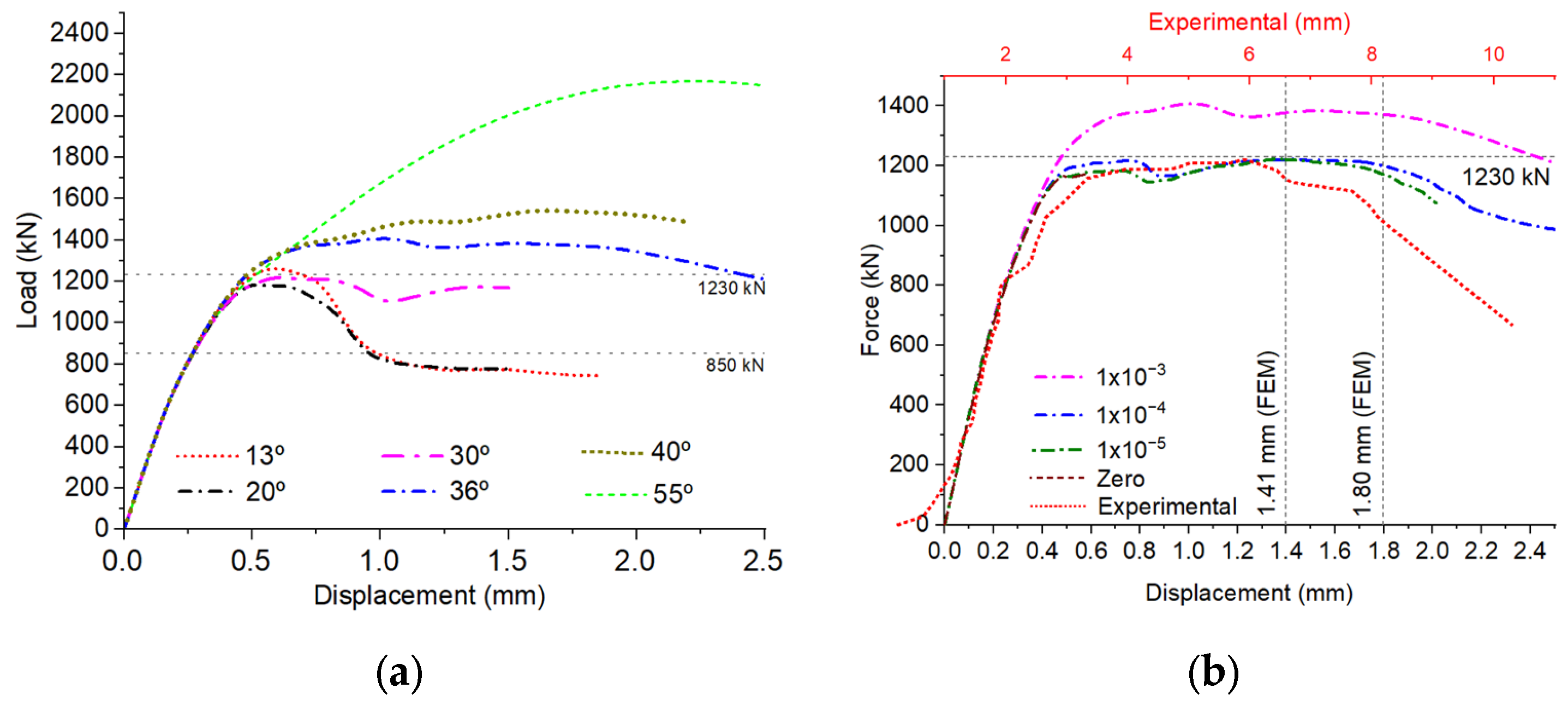
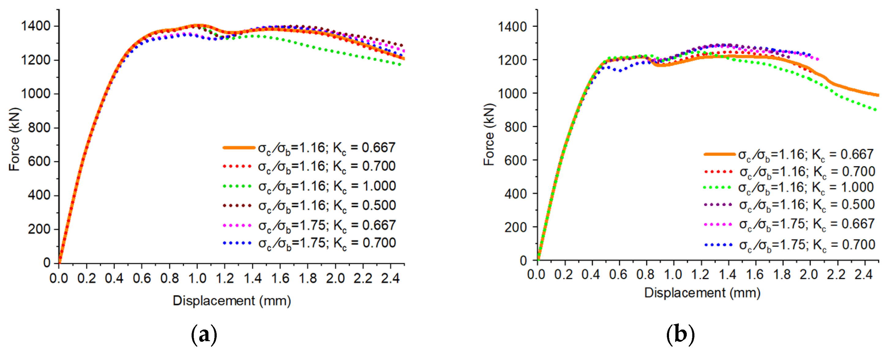
3.1.2. Influence of CDP Parameters on Force × Displacement Curves

Static Analysis

The influence of $\psi$ and $\mu$ parameters resulted in curves of Figure 6a and Figure 6b, respectively. Due to the greater stiffness, displacement results are lower in numerical models. In spite of that, the curve behavior was in agreement with the results of Chan and Poh [5] considering the yielding plateau presented. For the representation of the experimental behavior, a scale adjustment was adopted (red axis in the graph) so that it could be compatible with numerical curves (Figure 6b).

Reinforced concrete beams with low ψ values resulted in a loss of ductility [20] and were not sensitive to bending behavior [54]. For numeric models of four-pile caps, greater values of ψ resulted in a significant increase in peak force values without influencing the initial branch.

Flexural failure of four-pile caps as a consequence of excessive yielding of tie steel reinforcement produced displacements without an increase in ultimate force [3], which agrees with the results of Chan and Poh [5]. Melendez et al.’s results [57] also exhibit flexural failure for this case. Based on these factors and the recommended value of ψ, the value of 36° was adopted to analyze other parameters’ influence.

Models with different values of ${\sigma }_c/{\sigma }_b$ ratio and $K_c$ present a difference of less than 1.5% in ultimate load when μ is equal to 1 × 10⁻⁴ and 1 × 10⁻⁵. This fact enables the adoption of μ equal to 1 × 10⁻⁴ as it guarantees a precise failure force with lower computational cost.

Figure 7 illustrates the force × displacement curves for ψ equal to 36° with the extrapolation of ${\sigma }_b/{\sigma }_c$ and $K_c$. Models were processed with μ equal to 1 × 10⁻³ (Figure 7a) and 1 × 10⁻⁴ (Figure 7b), while $ϵ$ was assumed to be equal to 0.1.

When $K_c$ was equal to 1.0, the results showed to be independent of μ, as demonstrated in the literature [23]. Thus, the material softening after peak load approximates a brittle behavior, which is intensified when $\mu$ is equal to 1 × 10⁻⁴.

In the case of extrapolated values of larger ${\sigma }_b/{\sigma }_c$, an impact was observed in the yielding plateau, which takes place with a lower force. In addition, when this ratio was assumed to be equal to 1.75, the peak load was larger. It was also observed that when $\mu$ was equal to 1 × 10⁻⁴, this influence was more significant.

Table 4. Peak load results of static analysis numerical models.

${\mathit{\sigma }}_{\mathit{c}}/{\mathit{\sigma }}_{\mathit{b}}$	Kc	μ	${\mathit{F}}_{\mathit{C}\mathit{D}\mathit{P}}$ (kN)	$\uparrow \left(\mathbf{\%}\right)$	(mm)	$\frac{{\mathit{F}}_{\mathit{C}\mathit{D}\mathit{P}}}{{\mathit{F}}_{\mathit{e}\mathit{x}\mathit{p}\mathit{e}\mathit{r}\mathit{i}\mathit{m}\mathit{e}\mathit{n}\mathit{t}\mathit{a}\mathit{l}}}$
1.16	0.667	1 × 10−5	1220.61	-	1.39	0.992
		1 × 10−4	1221.84	0.10	1.43	0.993
		1 × 10−3	1406.81	15.25	1.02	1.143
	0.700	1 × 10−5	1241.27	-	1.34	1.009
		1 × 10−4	1245.59	1.40	1.41	1.012
		1 × 10−3	1405.07	13.56	1.02	1.142
1.75	0.667	1 × 10−5	1279.80	-	1.38	1.040
		1 × 10−4	1281.00	0.09	1.29	1.041
		1 × 10−3	1397.88	9.23	1.57	1.136
	0.700	1 × 10−5	1283.58	-	1.31	1.043
		1 × 10−4	1286.27	0.02	1.37	1.045
		1 × 10−3	1399.35	9.01	1.57	1.137
Obs.: For all models, $\psi$ = 36° and $ϵ$ = 0.1.

summarizes the results obtained from the numeric models in terms of force × displacement at the peak of the curve. The percentage column indicates the force increase relative to the numeric model when $\mu$ equals 1 × 10⁻⁵. Additionally, the experimental peak load was 1230 kN.

Thus, the selection criteria for input parameter values in simulations for both solvers were based on the convergence of numeric to experimental results and computational effort. The model that presented the best agreement to the experimental displacement and failure load was chosen. These values are highlighted in Table 4.

Quasi-Static Analysis

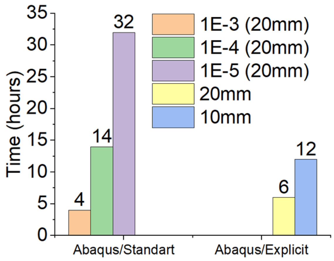
Extrapolation of $\psi$ with recommended values of ${\sigma }_c/{\sigma }_b$ and $K_c$ resulted in the curves presented in Figure 8a. It was assigned a mesh size of 20 mm, which led to a peak force closer to that in the experiment. For the model with a $\psi$ value of 55°, the results indicated only a substantial increase in ductility without a significant increase in peak load.

The values of peak load were influenced by approximately 5.0~8.0% due to the extrapolation of ${\sigma }_c/{\sigma }_b$ and $K_c$ (Figure 8b). Figure 9a illustrates the behavior of the force × displacement curves so that the need for a refined mesh in quasi-static analysis could be highlighted. The curve with a 20 mm mesh and ψ equal to 55° did not show the plateau of the experimental curve. There was a need for mesh refinement due to the value of $\psi$ being close to the upper limit. The model with a 10 mm mesh and 55° angle resulted in an excessive gain in ultimate load, and with a new calibration of $\psi$, it was verified that the value of 45° presented satisfactory results compared to the experimental curve.

The CDP parameters adopted had a similar influence on results as in the ABAQUS^®/Standard mode. However, the Explicit solver exhibited an initial branch with a higher load (dotted lines—Figure 9); at the same time, it presented a lower stiffness than the Standard solver.

Table 5. Force × displacement values by quasi-static analysis.

$\mathit{\psi }$	${\mathit{\sigma }}_{\mathit{c}}/{\mathit{\sigma }}_{\mathit{b}}$	Kc	${\mathit{F}}_{\mathit{C}\mathit{D}\mathit{P}}$ (kN)	$\uparrow \left(\mathbf{\%}\right)$	(mm)	$\frac{{\mathit{F}}_{\mathit{C}\mathit{D}\mathit{P}}}{{\mathit{F}}_{\mathit{e}\mathit{x}\mathit{p}}}$
Mesh size 20 mm
55	1.16	0.667	1202.79	-	0.84	0.977
		0.700	1213.29	0.87	0.79	0.986
	1.75	0.667	1235.55	-	1.06	1.004
		0.700	1237.81	0.18	1.06	1.006
Mesh size 10 mm
55	1.16	0.667	1788.65	-	1.49	1.450
45	1.16	0.500	1371.20	-	0.66	1.114
		0.667	1342.40	-	0.66	1.091
		1.000	1372.78	-	0.66	1.116
	1.75	0.500	1323.60	-	1.34	1.073
		0.667	1320.55	-	1.34	1.073
		1.000	1319.40	-	1.34	1.072

summarizes the results obtained through quasi-static analysis. Values in bold were chosen for comparison with static analysis.

Computational Cost

The adoption of $\mu$ values equal to 1 × 10⁻³, 1 × 10⁻⁴, and 1 × 10⁻⁵ results in similar curves. But, Figure 10 indicated that $\mu$ values equal to 1 × 10⁻⁵ and 1 × 10⁻⁴ presented a significant increase in simulation time than when $\mu$ was assumed to be 1 × 10⁻³.

The cap with a 20 mm mesh size comprised 48.976 elements and 53.837 nodes, while the 10 mm mesh size included 430.696 elements and 411.041 nodes. It is important to note that these values account only for the cap instance.

The static analysis’s computational effort was 12.244, 3.489, and 1.530 elements per hour when μ was equal to 1 × 10⁻³, 1 × 10⁻⁴, and 1 × 10⁻⁵, respectively, versus 34.253 elements per hour with quasi-static analysis. The time estimation can be obtained from these values. However, the results may be influenced by the number of points provided in the uniaxial curves of stress × strain × damage.

Regarding the computational cost, quasi-static displayed a similar average time compared to static analysis with μ equal to 1 × 10⁻⁴. Furthermore, a μ value equal to 1 × 10⁻⁴ for the static analysis is recommended.

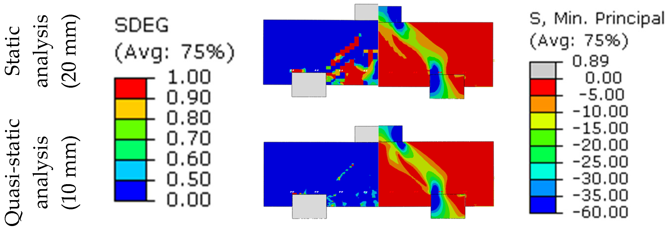
3.1.3. Compressive Stresses and Concrete Damage

The stress flow and DAMACEC ($d_c$), DAMAGET ($d_t$), and SDEG variables were analyzed for models with parameter values highlighted in Table 4 and Table 5. For this analysis, a 45° section cut connecting two piles was traced in the cap. It is worth noting that the SDEG variable results from a combination of DAMAGET and DAMAGEC.

Figure 11 presents the compressive stress flow (negative sign) and SDEG result for comparison between solvers. Subsequently, results point to a correlation between SDEG and the DAMAGET (Figure 12), which influenced the compressive stress flow. In addition, due to the need for mesh refinement, the quasi-static solver was identified to have lower dispersion.

In the literature, the upper face of the piles for two-pile cap [56], four-pile cap [6], and six-pile cap [7] presented stress concentration. The numeric models that simulated Chan and Poh’s [5] experiments exhibited this concentration. However, in the case of the numeric model based on Suzuki, Otsuki, and Tsubata’s [3] experiment, this behavior occurs in different ways, as discussed in Section 3.2.

The experiments are more accurately simulated when considering concrete tensile strength [13]. Furthermore, the origin of cracks in the strut’s lower-central region can be attributed to tensile stress in concrete due to the progress of compressive stress flow, an effect identified in an experimental study from the literature [65]. Numeric models considered in this section and illustrated in Figure 12 correlate and compare this behavior between solvers.

The results between solvers were comparable. Furthermore, the specimen analyzed failed in flexure, and the results of both solvers presented a compressive stress flow with well-defined contour diagrams, as expected.

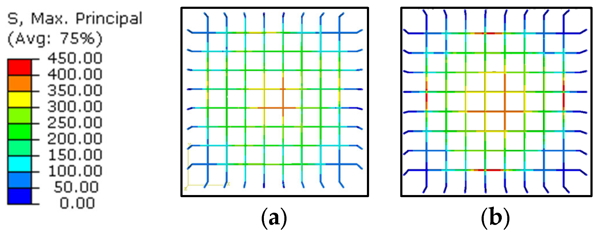
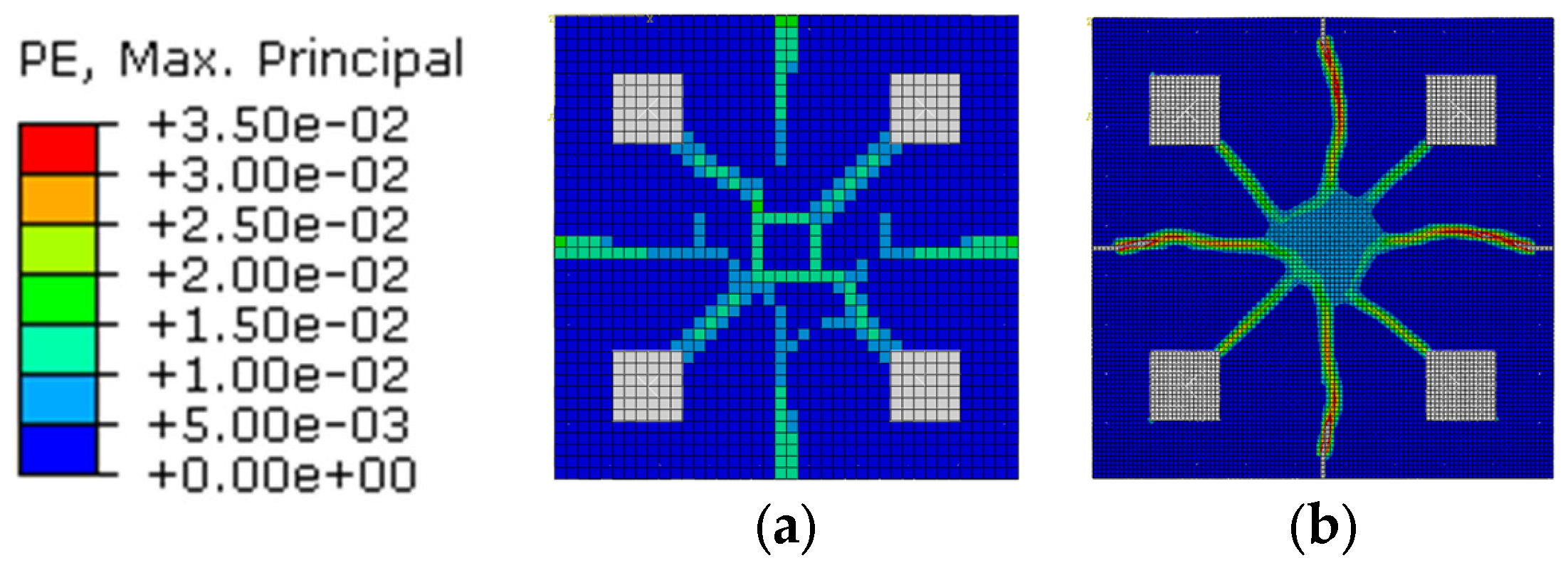
3.1.4. Reinforcement Stress and Cracking Pattern

The research did not find studies that compared the results of numeric and experimental reinforcement stress. In such a manner, these studies considered the compatibility of force × displacement curves enough to simulate mechanical behavior. According to Chan and Poh’s [5] experiments, the reinforcement yielded at the specimen’s peak force. Figure 13 illustrates the stresses of reinforcement displayed in the numeric models.

Differently from the experiments, the yielding of reinforcement bars was not observed in numeric models (Table 2). In the case of a quasi-static analysis, the stress in reinforcement reached higher values than those observed in static analysis. Despite this, the crack pattern of these numeric models is similar, according to Figure 14.

These results highlighted the difficulty in simulating the behavior of pile caps. One factor that contributed to this is the higher stiffness of numeric models due to the perfect bond between reinforcement and concrete. However, the numerical model based on Suzuki, Otsuki, and Tsubata’s work [3] presented reinforcement tensile values similar to those of the experimental campaign, as discussed in Section 3.2.

3.2. Specimen of Suzuki, Otsuki, and Tsubata (1998)

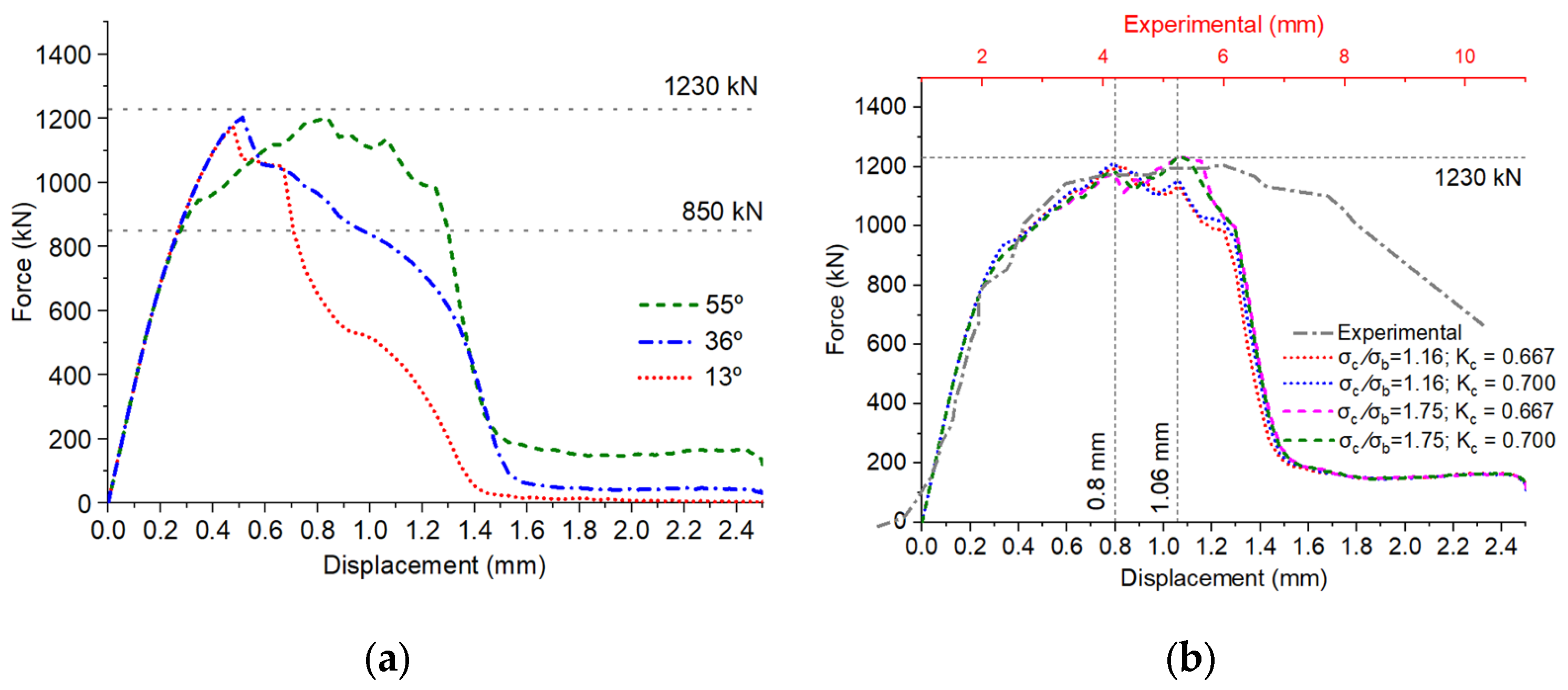
3.2.1. Calibration of Force × Displacement Curve

Initial ψ values adopted in the static and quasi-static analysis were 36° and 50°, respectively. The mesh size result is equal to the previous analysis of Chan and Poh [5].

Due to doubts regarding the diameter of the aggregate used in the experimental campaign, the extrapolation of properties to define the uniaxial force × strain curve was executed, as presented in Section 2.3. These properties were validated according to the maximum damage associated with elements and aggregate diameter. Values in parentheses ($d_{max}$/$d_t$) refer to the aggregate diameter ($d_{max}$) and the maximum value of tensile damage considered in the curve ($d_t$). The results are presented in Figure 15.

In this case, it can be seen that the numerical and experimental curves matched. One factor that can influence this result is the degree of freedom of supports in the horizontal direction, which is the only difference from the numeric model simulated previously. This highlights the necessity of the experimental setup to consider measuring displacement and rotation of supports for accurate numeric models.

The range of displacement from 0.2 to 0.4 mm and from 0.6 to 0.8 mm for static and quasi-static analysis presented a perturbation in the plotted curve. Experimental results indicated that the reinforcement yielded at 1029 kN, and the shear failure occurred at 1039 kN. Static analysis indicated a fine convergence for the assumed values of aggregate diameter, highlighting the necessity of information about the material used for mixing concrete. The quasi-static analysis did not present agreement with the correct values of the diameter aggregate.

Although the plotted curve with $d_{max}$ of 25 mm agrees with the experimental curve for the static analysis, this adoption led to a higher peak load. This agrees with previous research that showed the concrete tensile strength affects the strength capacity of the numeric model [18]. In addition, it also agrees with the results of this paper that presented a numerical peak force with a larger value. Models processed with 80% DAMAGET were affected in a similar manner. Quasi-static analysis was more sensitive for extrapolated values of concrete tensile strength, resulting in conservative predictions.

Altering values of CDP parameters resulted in a similar influence for both solvers. In the case of ${\sigma }_c/{\sigma }_b$ and $K_c$, the influence on curves agrees with the shear wall results [23].

Table 6. Force × displacement of simulation based on BPC-30-30.

$\mathit{\psi }$	${\mathit{\sigma }}_{\mathit{c}}/{\mathit{\sigma }}_{\mathit{b}}$	${\mathit{K}}_{\mathit{c}}$	$\mathit{\mu }$	${\mathit{d}}_{\mathit{m}\mathit{a}\mathit{x}}$	${\mathit{d}}_{\mathit{t}}$	Mesh Size (mm)	$\mathit{F}$(kN)	(mm)	$\frac{\mathit{F}}{{\mathit{F}}_{\mathit{e}\mathit{x}\mathit{p}}}$
-	-	-	-	-	-	Experimental	1034.00	~2.00	1.000
Static analysis
36	1.16	0.667	1 × 10−5	10	95	20	1024.82	1.70	0.991
36	1.16	0.667	1 × 10−5	10	80	20	1178.93	1.58	1.140
36	1.16	0.667	1 × 10−5	25	95	20	1106.62	1.56	1.070
36	1.16	0.667	1 × 10−4	25	95	20	1050.36	1.34	1.016
36	1.75	0.667	1 × 10−5	10	95	20	1048.64	1.87	1.014
36	1.75	0.667	1 × 10−5	25	95	20	1116.02	1.71	1.079
36	1.75	1.000	1 × 10−5	10	95	20	1069.18	1.96	1.034
30	1.75	0.667	1 × 10−4	25	95	20	1021.80	1.51	0.988
Quasi static analysis
36	1.16	0.667	-	10	95	20	768.80	0.79	0.743
50	1.16	0.667	-	10	95	10	1071.61	1.60	1.036
50	1.16	0.667	-	10	80	10	1492.81	1.77	1.445
50	1.16	0.667	-	25	95	10	1206.33	0.88	1.165
50	1.75	0.667	-	25	95	10	1190.58	1.00	1.150
50	1.75	0.667	-	10	95	10	1080.55	1.52	1.045

summarizes the peak force and respective displacement values for processed models. Bolded values were selected for the analyses of mechanical behavior in both analysis methods.

3.2.2. Compressive Stresses and Concrete Degradation

Analogous to previous simulations in this work, Figure 16 presents the values of SDEG and compressive stress (MPa) for the models highlighted in Table 6. Due to the similarity of SDEG with values of DAMAGET for this case, the DAMAGET results were not displayed.

In this case, stress concentration occurs differently when compared to simulations based on Chan and Poh’s data [5]. A plausible explanation for this result can be related to the boundary conditions of supports, as their stiffness influences stress concentration [7]. Furthermore, Figure 11 indicates a more conservative stress diagram for the static analysis. This result can be associated with the static analysis’s accuracy in capturing the type of failure for the specimens of Suzuki, Otsuki, and Tsubata (concrete failure after reinforcement yielding).

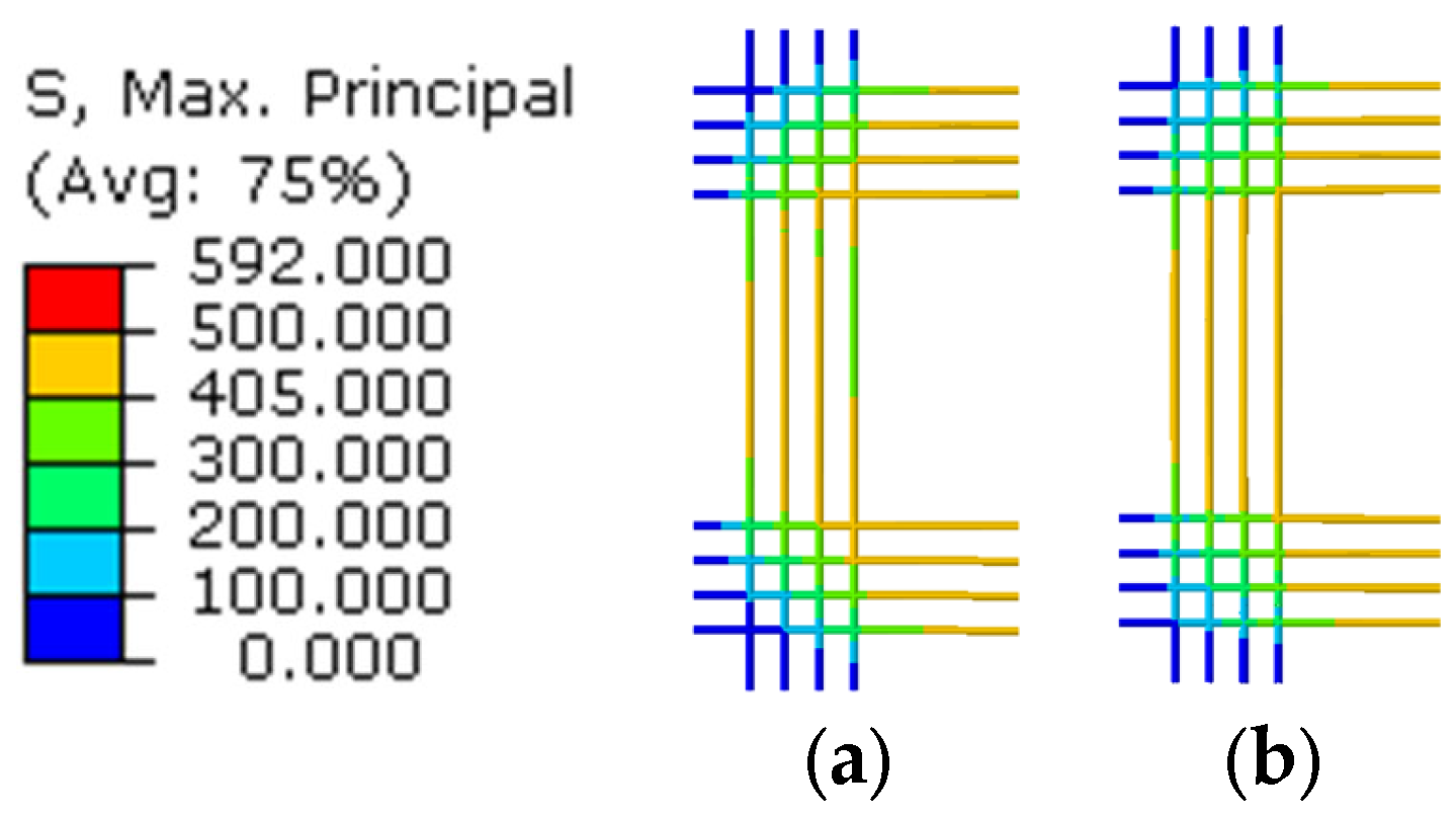
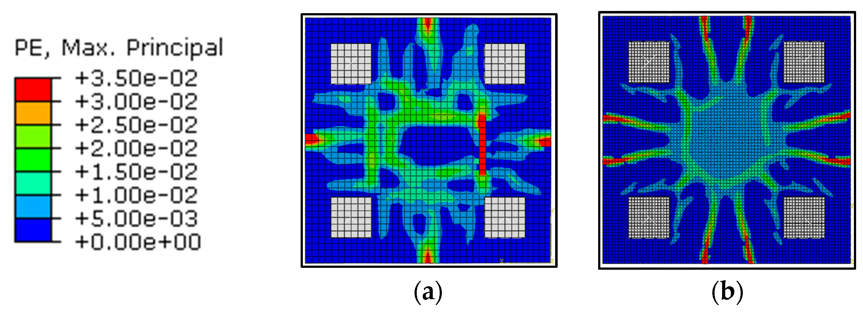
3.2.3. Reinforcement Stress and Cracking Pattern

Suzuki, Otsuki, and Tsubata [3] did not measure the deformation of the reinforcement; however, the numerical models with different solvers presented similar stresses for reinforcement. Figure 17 exhibits these results.

Suzuki, Otsuki, and Tsubata’s specimens failed due to shear stress after the yielding of reinforcement, with cracks around piles [3]. The cracking pattern of this experimental failure mode was well reproduced in numerical models (Figure 18).

According to the illustrated results, the quasi-static analysis shows larger stresses in reinforcements, which can be influenced by the refined mesh or characteristics of the solver. Despite this, both analysis methods agreed well with the experimental results showing the yielding of reinforcement, which also agrees with the values calculated in the proposal of Melendez et al. [57].

3.3. Feasibility of Solvers for Extrapolated Numerical Models

For geometrically extrapolated numeric models,

Table 7. Prediction of peak loads of extrapolated models.

Model	${\mathit{F}}_{\mathit{M}\mathit{e}\mathit{l}}$ (kN)	${\mathit{F}}_{\mathit{S}\mathit{t}\mathit{d}}$ (kN)	${\mathit{F}}_{\mathit{E}\mathit{x}\mathit{p}\mathit{l}\mathit{i}\mathit{c}\mathit{i}\mathit{t}}$ (kN)	$\frac{{\mathit{F}}_{\mathit{S}\mathit{t}\mathit{d}}}{{\mathit{F}}_{\mathit{M}\mathit{e}\mathit{l}}}$	$\frac{{\mathit{F}}_{\mathit{E}\mathit{x}\mathit{p}\mathit{l}\mathit{i}\mathit{c}\mathit{i}\mathit{t}}}{{\mathit{F}}_{\mathit{M}\mathit{e}\mathit{l}}}$
MCalibrate	942	1024	1071	1.08	1.13
MShear	1105	1139	1362	1.03	1.23
M25D50E	880	862	852	0.98	0.96
M25D45E	983	1059	1149	0.98	1.16
M25D37E	1170	1236	1325	1.05	1.13
M28D50E	1004	1028	1081	1.02	1.07
M28D45E	1107	1123	793	1.01	0.71
M28D38E	1284	1351	1068	1.05	0.83
M32D50E	1108	1151	919 *	1.04	0.79
M32D45E	1212	1306	986 *	1.08	0.81
M32D37E	1375	1406	1085 *	1.02	0.79
			AVG	1.03	0.96
			SD	0.03	0.19
			CV(%)	3.29	19.18

* Flexural failure.

presents the results of peak force for static ($F_{Std}$) and quasi-static ($F_{Explicit}$) analysis, which are compared to the predicted rupture load in the proposal of Melendez et al. [57] ($F_{Mel}$). These ratios were then compared to the ratios of the calibrated model.

The quasi-static analysis results are not in agreement with the predicted values of static analysis. Additionally, the quasi-static analysis showed to be highly sensitive to the increased area of reinforcement and different geometric dimensions of the pile cap. More critical results are obtained in M32 models, which exhibited a different failure mode. On the other hand, the peak forces of the static analysis agree well with predicted values ($F_{Mel}$).

4. Conclusions

The results obtained in this research make it possible to conclude the following:

• The CDP model presented favorable conditions for the numerical simulation of volumetric elements based on the case of the four-pile caps investigated.
• Regarding the modes or methods of analysis, it was found that the results of both solvers were equally sensitive to ${\sigma }_{b0}/{\sigma }_{c0}$ and $K_c$ parameters. This makes it possible to adopt the values recommended in the literature, that is, equal to 1.16 and 0.667, respectively. In the case of the parameter $\psi$, for the “quasi-static” analysis mode, the results were greater and different in the calibrated models (45° and 50°). This result suggests that a calibration has to be carried out for its definition. For the “static” analysis mode, values of ψ and μ equal to 36° and 1 × 10⁻⁴, respectively, are recommended.
• The values of CDP parameters did not influence the initial branch of the force × displacement curve. However, the tensile stress × strain relation of concrete showed a greater influence on the calibration of the curve. In this case, it is important to highlight the need for the correct specification of materials for the definition of the uniaxial concrete tensile curve. It is also important due to the proper definition of 95% tensile damage which influences the ultimate load of the models.
• Regarding the computational cost of the analyzed models, the “quasi-static” analysis mode did not present benefits compared to the “static” analysis when $\mu$ was equal to 1 × 10⁻⁴. This occurred due to the need for a refined mesh in the “quasi-static” method.
• Both analysis modes using CDP produced models that presented fine agreement with the experimental force × displacement curves. However, the “static” analysis simulates more precisely the stress contour diagrams for specimens with shear failure (concrete splitting), which can be seen as a strut with intensified damage.
• In the calibration of force × displacement curves, problems were identified, and the reason for these can be associated with the absence of data from experimental tests. In this case, the boundary condition description showed to be crucial. Furthermore, the stress concentration over piles was similar in both solvers; however, the stress accuracy differs between the types of specimens investigated, which can be attributed to boundary condition considerations. This result highlights the necessity of standardizing the experimental setup.
• In the parametric study of geometrical parameters, the “quasi-static” analysis did not present a good correlation in the estimated values, indicating the need for studies for the identification of factors that led to this behavior. The coefficients of variation, obtained with results from the proposal by Melendez et al. [57], were 3.29% and 19.18% for the “static” and “quasi-static” analysis modes, respectively.

Overall, the use of solvers with viscoplastic regularization is recommended in the simulation of four-pile caps. It is suggested especially when conducting a parametric study with geometrical parameters.

References

1. Blévot, J.; Frémy, R. Annales de l’Institut Technique du Batiment et des Travaux Publics; Institut Technique du Bâtiment et des Travaux Publics: Paris, France, 1967; Volume 20, pp. 223–295. [Google Scholar]
2. ABNT NBR 6118. NBR 6118; Design of Concrete Structures—Procedure. Associação Brasileira de Normas Técnicas (ABNT): Rio de Janeiro, Brazil, 2023; Volume 238. (In Portuguese)
3. Suzuki, K.; Otsuki, K.; Tsubata, T. Influence of Bar Arrangement on Ultimate Strength of Four-Pile Caps. Trans. Japan Concr. Inst. 1998, 20, 195–202. [Google Scholar]
4. Clarke, J.L. Behaviour and Design of Pile Caps with Four Piles; Technical; Cement and Concrete Association: London, UK, 1973; p. 489. [Google Scholar]
5. Chan, T.K.; Poh, C.K. Behaviour of precast reinforced concrete pile caps. Constr. Build. Mater. 2000, 14, 73–78. [Google Scholar] [CrossRef]
6. Miguel-Tortola, L.; Miguel, P.F.; Pallarés, L. Strength of pile caps under eccentric loads: Experimental study and review of code provisions. Eng. Struct. 2019, 182, 251–267. [Google Scholar] [CrossRef]
7. Meléndez, C.; Miguel, P.F. Modelling Boundary Conditions Imposed by Loads and Supports in 3D D-Regions. Computational Modelling of Concrete Structures; CRC Press: Boca Raton, FL, USA, 2018; pp. 679–688. [Google Scholar] [CrossRef]
8. Sam, C.; Iyer, P.K. Nonlinear finite element analysis of reinforced concrete four-pile caps. Comput. Struct. 1995, 57, 605–622. [Google Scholar] [CrossRef]
9. Nogueira, T.B.; Souza, R.A. de Análise, dimensionamento e verificaçao de elementos espaciais em concreto armado utilizando o método dos elementos finitos e o método das bielas. Rev. Int. Metod. Numer. Para Calc. Disen. Ing. 2006, 22, 31–44. [Google Scholar]
10. Delalibera, R.G.; Sousa, G.F. Numerical analyses of two-pile caps considering lateral friction between the piles and soil. Rev. IBRACON Estrut. e Mater. 2021, 14, e14604. [Google Scholar] [CrossRef]
11. Gonçalves, V.F.; Delalibera, R.G.; de Oliveira Filho, M.A. Analysis of the pile-to-cap connection of pile caps on two steel piles—An experimental and numerical study. Eng. Struct. 2022, 252, 113629. [Google Scholar] [CrossRef]
12. Buttignol, T.E.T.; Almeida, L.C. Concrete compressive characteristic strength analysis of pile caps with three piles. Rev. IBRACON Estrut. Mater. 2013, 6, 158–177. [Google Scholar] [CrossRef]
13. Oliveira, D.S.; Barros, R.; Giongo, J.S. Blocos de concreto armado sobre seis estacas: Simulação numérica e dimensionamento pelo método de bielas e tirantes. Rev. IBRACON Estrut. Mater. 2014, 7, 1–23. [Google Scholar] [CrossRef]
14. Bloodworth, A.G.; Cao, J.; Xu, M. Numerical Modeling of Shear Behavior of Reinforced Concrete Pile Caps. J. Struct. Eng. 2012, 138, 708–717. [Google Scholar] [CrossRef]
15. Randi, R.P.; Almeida, L.C.; Trautwein, L.M.; Munhoz, F.S. Análise da influência do comprimento de ancoragem da armadura do pilar no bloco sobre duas estacas. Rev. IBRACON Estrut. e Mater. 2018, 11, 1122–1150. [Google Scholar] [CrossRef]
16. Munhoz, F.S. Análise Experimental e Numérica de Blocos Rígidos Sobre duas Estacas com Pilares de Seções Quadradas e Retangulares e Diferentes Taxas de Armadura; Digital Library of Intellectual Production of Universidade de São Paulo: São Paulo, Brazil, 2014; p. 358. [Google Scholar]
17. Luchesi, G.L.; Randi, R.d.P.; Trautwein, L.M.; Almeida, L.C.D. Important aspects in experimental versus numerical comparative analysis in pile caps. Rev. IBRACON Estrut. Mater. 2022, 15, e15502. [Google Scholar] [CrossRef]
18. Meléndez, C.; Miguel, P.F.; Pallarés, L. A simplified approach for the ultimate limit state analysis of three-dimensional reinforced concrete elements. Eng. Struct. 2016, 123, 330–340. [Google Scholar] [CrossRef]
19. Basha, A.; Tayeh, B.A.; Maglad, A.M.; Mansour, W. Feasibility of improving shear performance of RC pile caps using various internal reinforcement configurations: Tests and finite element modelling. Eng. Struct. 2023, 289, 116340. [Google Scholar] [CrossRef]
20. Earij, A.; Alfano, G.; Cashell, K.; Zhou, X. Nonlinear three–dimensional finite–element modelling of reinforced–concrete beams: Computational challenges and experimental validation. Eng. Fail. Anal. 2017, 82, 92–115. [Google Scholar] [CrossRef]
21. Hafezolghorani, M.; Hejazi, F.; Vaghei, R.; Jaafar, M.S.B.; Karimzade, K. Simplified damage plasticity model for concrete. Struct. Eng. Int. 2017, 27, 68–78. [Google Scholar] [CrossRef]
22. Sümer, Y.; Aktaş, M. Defining parameters for concrete damage plasticity model. Chall. J. Struct. Mech. 2015, 1, 149–155. [Google Scholar] [CrossRef]
23. Silva, L.M.E.; Christoforo, A.L.; Carvalho, R.C. Calibration of concrete damaged plasticity model parameters for shear walls. Rev. Mater. 2021, 26, e12944. [Google Scholar] [CrossRef]
24. Rainone, L.S.; Tateo, V.; Casolo, S.; Uva, G. About the Use of Concrete Damage Plasticity for Modeling Masonry Post-Elastic Behavior. Buildings 2023, 13, 1915. [Google Scholar] [CrossRef]
25. Simulia Abaqus 6.11 Theory Manual; Dassault Systèmes Simulia Corp.: Providence, RI, USA, 2017; Volume IV, p. 1172.
26. Ali, A.; Kim, D.; Cho, S.G. Modeling of nonlinear cyclic load behavior of I-shaped composite steel-concrete shear walls of nuclear power plants. Nucl. Eng. Technol. 2013, 45, 89–98. [Google Scholar] [CrossRef]
27. Dawood, H.; ElGawady, M.; Hewes, J. Behavior of Segmental Precast Posttensioned Bridge Piers under Lateral Loads. J. Bridg. Eng. 2012, 17, 735–746. [Google Scholar] [CrossRef]
28. Dong, Y.R.; Xu, Z.D.; Zeng, K.; Cheng, Y.; Xu, C. Seismic behavior and cross-scale refinement model of damage evolution for RC shear walls. Eng. Struct. 2018, 167, 13–25. [Google Scholar] [CrossRef]
29. Genikomsou, A.S.; Polak, M.A. Finite element analysis of punching shear of concrete slabs using damaged plasticity model in ABAQUS. Eng. Struct. 2015, 98, 38–48. [Google Scholar] [CrossRef]
30. Milligan, G.J.; Polak, M.A.; Zurell, C. Finite element analysis of punching shear behaviour of concrete slabs supported on rectangular columns. Eng. Struct. 2020, 224, 111189. [Google Scholar] [CrossRef]
31. Husain, M.; Eisa, A.S.; Hegazy, M.M. Strengthening of reinforced concrete shear walls with openings using carbon fiber-reinforced polymers. Int. J. Adv. Struct. Eng. 2019, 11, 129–150. [Google Scholar] [CrossRef]
32. Jha, S.; Roshan, A.D.; Bishnoi, L.R. Floor response spectra for beyond design basis seismic demand. Nucl. Eng. Des. 2017, 323, 259–268. [Google Scholar] [CrossRef]
33. Kaushik, S.; Dasgupta, K. Seismic behavior of slab-structural wall junction of RC building. Earthq. Eng. Eng. Vib. 2019, 18, 331–349. [Google Scholar] [CrossRef]
34. Li, C.; Hao, H.; Bi, K. Numerical Study on the Seismic Performance of Precast Segmental Concrete Columns under Cyclic Loading. Eng. Struct. 2017, 148, 373–386. [Google Scholar] [CrossRef]
35. Liu, J.; Yang, Y.; Liu, J.; Zhou, X. Experimental investigation of special-shaped concrete-filled steel tubular column to steel beam connections under cyclic loading. Eng. Struct. 2017, 151, 68–84. [Google Scholar] [CrossRef]
36. Michał, S.; Andrzej, W. Analysis of “d” regions of RC structures based on example of frame corners. AIP Conf. Proc. 2018, 1922, 130002. [Google Scholar] [CrossRef]
37. Najafgholipour, M.A.; Dehghan, S.M.; Dooshabi, A.; Niroomandi, A. Finite element analysis of reinforced concrete beam-column connections with governing joint shear failure mode. Lat. Am. J. Solids Struct. 2017, 14, 1200–1225. [Google Scholar] [CrossRef]
38. Pavlović, M.; Marković, Z.; Veljković, M.; Bucrossed, D.; Signevac, D. Bolted shear connectors vs. headed studs behaviour in push-out tests. J. Constr. Steel Res. 2013, 88, 134–149. [Google Scholar] [CrossRef]
39. Pelletier, K.; Léger, P. Nonlinear seismic modeling of reinforced concrete cores including torsion. Eng. Struct. 2017, 136, 380–392. [Google Scholar] [CrossRef]
40. Ren, W.; Sneed, L.H.; Yang, Y.; He, R. Numerical Simulation of Prestressed Precast Concrete Bridge Deck Panels Using Damage Plasticity Model. Int. J. Concr. Struct. Mater. 2015, 9, 45–54. [Google Scholar] [CrossRef]
41. Surumi, R.S.; Jaya, K.P.; Greeshma, S. Modelling and Assessment of Shear Wall–Flat Slab Joint Region in Tall Structures. Arab. J. Sci. Eng. 2015, 40, 2201–2217. [Google Scholar] [CrossRef]
42. Vojdan, B.M.; Aghayari, R. Investigating the seismic behavior of RC shear walls with openings strengthened with FRP sheets using different schemes. Sci. Iran. 2017, 24, 1855–1865. [Google Scholar] [CrossRef]
43. Wang, M.Z.; Guo, Y.L.; Zhu, J.S.; Yang, X.; Tong, J.Z. Sectional strength design of concrete-infilled double steel corrugated-plate walls with T-section. J. Constr. Steel Res. 2019, 160, 23–44. [Google Scholar] [CrossRef]
44. Wei, M.W.; Richard Liew, J.Y.; Fu, X.Y. Nonlinear Finite Element Modeling of Novel Partially Connected Buckling-Restrained Steel Plate Shear Walls. Int. J. Steel Struct. 2019, 19, 28–43. [Google Scholar] [CrossRef]
45. Szczecina, M.; Winnicki, A. Relaxation Time in CDP Model Used for Analyses of RC Structures. Procedia Eng. 2017, 193, 369–376. [Google Scholar] [CrossRef]
46. Cuong-Le, T.; Minh, H.L.; Sang-To, T. A nonlinear concrete damaged plasticity model for simulation reinforced concrete structures using ABAQUS. Frat. Ed Integrita Strutt. 2021, 16, 232–242. [Google Scholar] [CrossRef]
47. Alfarah, B.; López-Almansa, F.; Oller, S. New methodology for calculating damage variables evolution in Plastic Damage Model for RC structures. Eng. Struct. 2017, 132, 70–86. [Google Scholar] [CrossRef]
48. Neuberger, Y.M.; Andrade, M.V.; de Sousa, A.M.D.; Bandieira, M.; da Silva Júnior, E.P.; dos Santos, H.F.; Catoia, B.; Bolandim, E.A.; de Moura Aquino, V.B.; Christoforo, A.L.; et al. Numerical Analysis of Reinforced Concrete Corbels Using Concrete Damage Plasticity: Sensitivity to Material Parameters and Comparison with Analytical Models. Buildings 2023, 13, 2781. [Google Scholar] [CrossRef]
49. Reginato, L.; de Sousa, A.M.D.; Santos, J.V.C.; El Debs, M.K. NLFEA of Reinforced Concrete Corbels: Proposed Framework, Sensibility Study, and Precision Level. Buildings 2023, 13, 1874. [Google Scholar] [CrossRef]
50. de Azevedo Palhares, R.; Weitzel Rossignoli, F.; Sales de Melo, G.; Jorge Nery de Lima, H. A numerical model capable of accurately simulating the punching shear behavior of a reinforced concrete slab. Struct. Concr. 2022, 23, 1134–1150. [Google Scholar] [CrossRef]
51. Arthi, S.; Jaya, K. Seismic performance of precast shear wall-slab connection under cyclic loading: Experimental test vs. numerical analysis. Earthq. Eng. Eng. Vib. 2020, 19, 739–757. [Google Scholar] [CrossRef]
52. Hu, R.; Fang, Z.; Benmokrane, B. Nonlinear finite-element analysis for predicting the cyclic behavior of UHPC shear walls reinforced with FRP and steel bars. Structures 2023, 53, 265–278. [Google Scholar] [CrossRef]
53. Scamardo, M.; Zucca, M.; Crespi, P.; Longarini, N.; Cattaneo, S. Seismic Vulnerability Evaluation of a Historical Masonry Tower: Comparison between Different Approaches. Appl. Sci. 2022, 12, 11254. [Google Scholar] [CrossRef]
54. Nguyen, T.N.H.; Tan, K.H.; Kanda, T. Investigations on web-shear behavior of deep precast, prestressed concrete hollow core slabs. Eng. Struct. 2019, 183, 579–593. [Google Scholar] [CrossRef]
55. Madkour, H.; Maher, M.; Ali, O. Finite element analysis for interior slab-column connections reinforced with GFRP bars using damage plasticity model. J. Build. Eng. 2022, 48, 104013. [Google Scholar] [CrossRef]
56. Najafgholipour, M.A.; Sarhadi, F. A finite element study on the ultimate lateral drift capacity of interior reinforced concrete flat slab-column connections. Structures 2022, 46, 913–926. [Google Scholar] [CrossRef]
57. Meléndez, C.; Sagaseta, J.; Miguel, P.F.; Rubio, L.P. Refined three-dimensional strut-and-tie model for analysis and design of four-pile caps. ACI Struct. J. 2019, 116, 15–29. [Google Scholar] [CrossRef]
58. Comité Européen de Normalisation. Eurocode 2: Design of Concrete Structures—Part 1-1: General Rules and Rules for Buildings; British Standard Institution: London, UK, 2004; p. 1. [Google Scholar]
59. Kmiecik, P.; Kamiński, M. Modelling of reinforced concrete structures and composite structures with concrete strength degradation taken into consideration. Arch. Civ. Mech. Eng. 2011, 11, 623–636. [Google Scholar] [CrossRef]
60. Dudziak, S.; Jackiewicz-Rek, W.; Kozyra, Z. On the calibration of a numerical model for concrete-to-concrete interface. Materials 2021, 14, 7204. [Google Scholar] [CrossRef] [PubMed]
61. Nana, W.S.A.; Bui, T.T.; Limam, A.; Abouri, S. Experimental and Numerical Modelling of Shear Behaviour of Full-scale RC Slabs under Concentrated Loads. Structures 2017, 10, 96–116. [Google Scholar] [CrossRef]
62. Panahi, H.; Genikomsou, A.S. Comparative evaluation of concrete constitutive models in non-linear finite element simulations of slabs with different flexural reinforcement ratios. Eng. Struct. 2022, 252, 113617. [Google Scholar] [CrossRef]
63. Comité Euro-International du Béton. CEB-FIB-Model Code 1990: Design Code; Thomas Telford: London, UK, 1993. [Google Scholar]
64. Comité Euro-International du Béton. CEB-FIP-Model Code; Precast Prestressed Concrete Institute: Lausanne, Switzerland, 2010; Volume 2010. [Google Scholar]
65. Adebar, P.; Kuchma, D.; Collins, M.P. Strut-and-tie models for the design of pile caps: An experimental study. ACI Strucutural J. 1990, 87, 191–199. [Google Scholar] [CrossRef]
66. Lubliner, J.; Oliver, J.; Oller, S.; Oñate, E. A plastic-damage model for concrete. Int. J. Solids Struct. 1989, 25, 299–326. [Google Scholar] [CrossRef]
67. Lee, J.; Fenves, G.L. Plastic-Damage Model for Cyclic Loading of Concrete Structures. J. Eng. Mech. 1998, 124, 892–900. [Google Scholar] [CrossRef]
Figure 1. Specimens dimensions (a) Pile Cap A and (b) BPC 30-30.
Buildings 14 02066 g001
Figure 2. Constitutive models for concrete (a) compression and (b) tensile stress based on specimen of Pile Cap A [5] and for BPC 30-30 [3] mesh of (c) 10 mm and (d) 20 mm.
Buildings 14 02066 g002
Figure 3. Numeric models of (a) Pile Cap A and (b) BPC 30-30.
Buildings 14 02066 g003
Figure 4. Meshed numeric models of (a) static, (b) quasi-static analysis, and (c) reinforcement bars with 10 cm2; in one direction.
Buildings 14 02066 g004
Figure 5. Force x displacement curves obtained in mesh calibration with (a) static and (b) quasi-static for experiments of Pile Cap A.
Buildings 14 02066 g005
Figure 6. Force × displacement curves of the model with the extrapolation of (a) ψ and (b) μ with the best ψ fit (36°).
Buildings 14 02066 g006
Figure 7. Force × displacement curve of extrapolated σ b / σ c and K c for μ equal to (a) 1 × 10⁻³ and (b) 1 × 10⁻⁴.
Buildings 14 02066 g007
Figure 8. Extrapolation of (a) ψ and (b) σ c / σ b and K c when ψ = 55° in quasi-static analysis.
Buildings 14 02066 g008
Figure 9. Force × displacement curves of the numeric model refer to Pile Cap A specimens with (a) recalibrated ψ and (b) extrapolated values of σ c / σ b and K c .
Buildings 14 02066 g009
Figure 10. Average time of simulation according to adopted solvers.
Buildings 14 02066 g010
Figure 11. Section cut illustrating SDEG (left side) and compressive stress flow (right side).
Buildings 14 02066 g011
Figure 12. Damage tensile strength in numeric models by (a) static and (b) quasi-static analysis.
Buildings 14 02066 g012
Figure 13. Tensile stress (MPa) of reinforcement in numeric models through (a) static and (b) quasi-static analysis.
Buildings 14 02066 g013
Figure 14. Cracking pattern under the bottom cap surface for (a) static and (b) quasi-static analysis.
Buildings 14 02066 g014
Figure 15. Force × displacement curves of parametric modeling of (a) static and (b) quasi-static analysis.
Buildings 14 02066 g015
Figure 16. Concrete degradation (SDEG—left side) and compression stress (S, Min.—right side) for models in static and quasi-static analysis.
Buildings 14 02066 g016
Figure 17. Reinforcement tensile stress (MPa) of numerical models presented in (a) static and (b) quasi-static analysis.
Buildings 14 02066 g017
Figure 18. Cracking pattern of models for (a) static and (b) quasi-static analysis.
Buildings 14 02066 g018