
Research on the Spatiotemporal Pattern and Influencing Mechanism of Coastal Urban Vitality: A Case Study of Bayuquan

Abstract
:1. Introduction
2. Literature Review
3. Materials and Methods
3.1. Materials
3.1.1. Study Area
3.1.2. Data
3.1.3. Variables
3.2. Framework and Study Design
3.3. Methods
3.3.1. Spatial Autocorrelation Analysis
3.3.2. Spatial Econometric Models
3.3.3. Geographically Weighted Regression Model
4. Results
4.1. Spatiotemporal Analysis of Coastal City Vitality
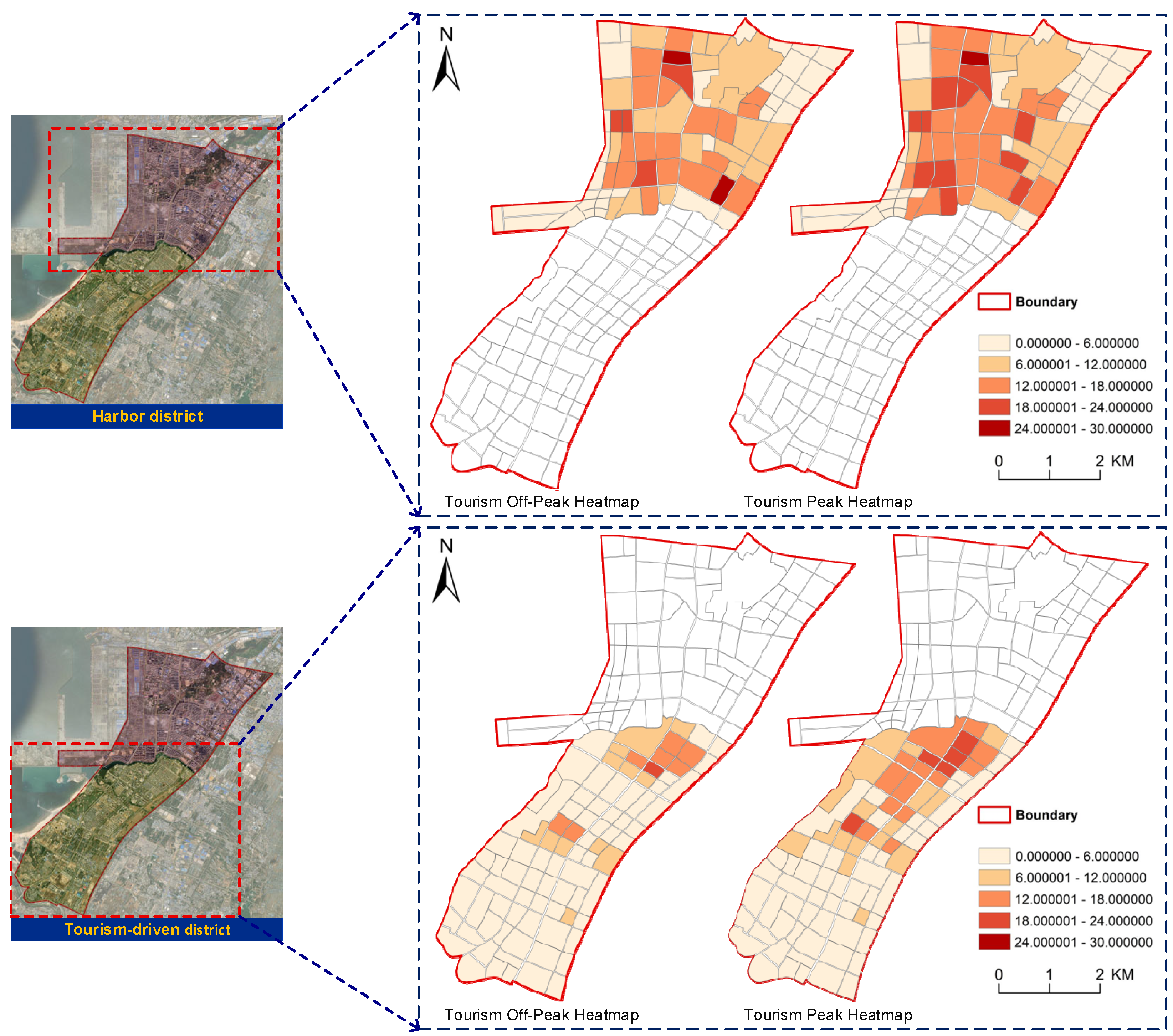
4.1.1. Vitality Space Difference Analysis
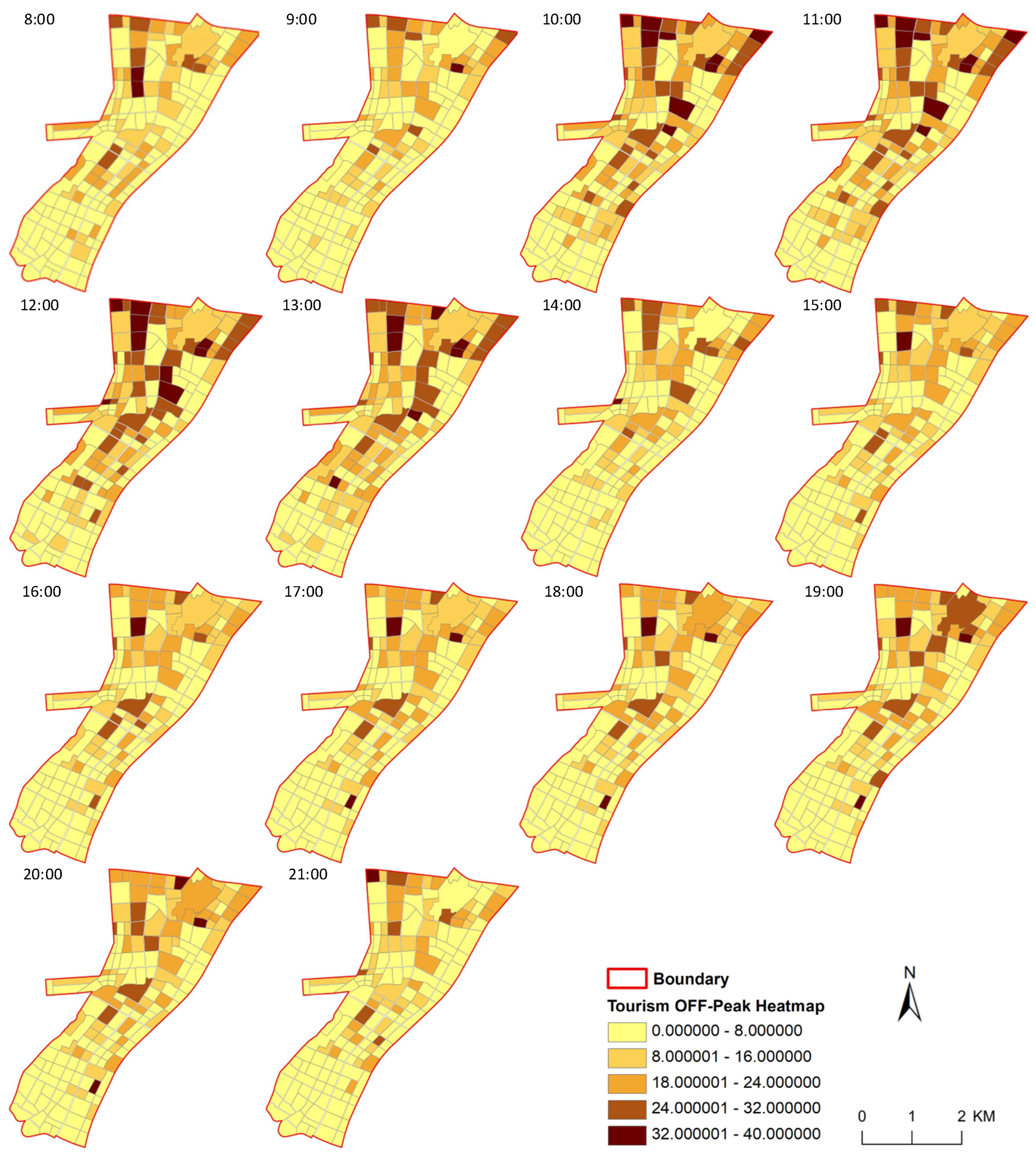
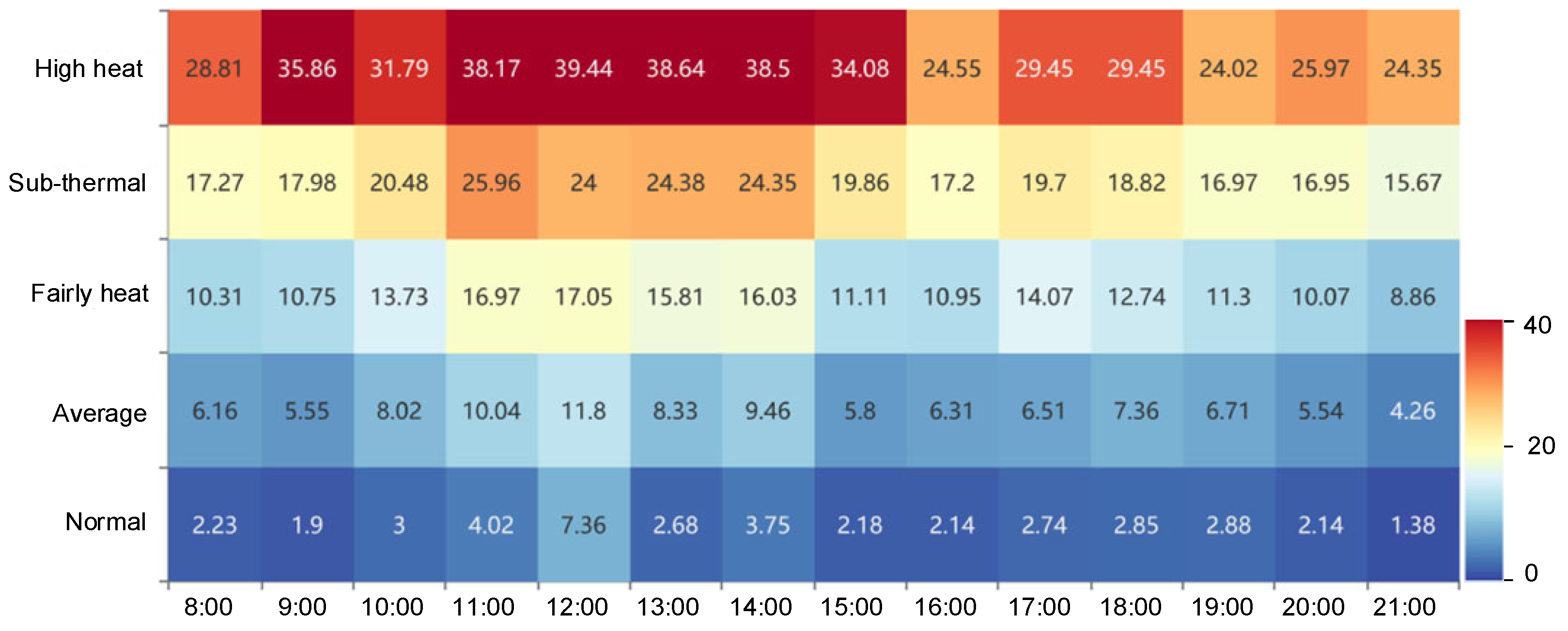
4.1.2. Vitality Time Variability Analysis
4.2. Impact of Coastal Space Construction on Vitality
4.2.1. Modeling Tests of Vitality Effects
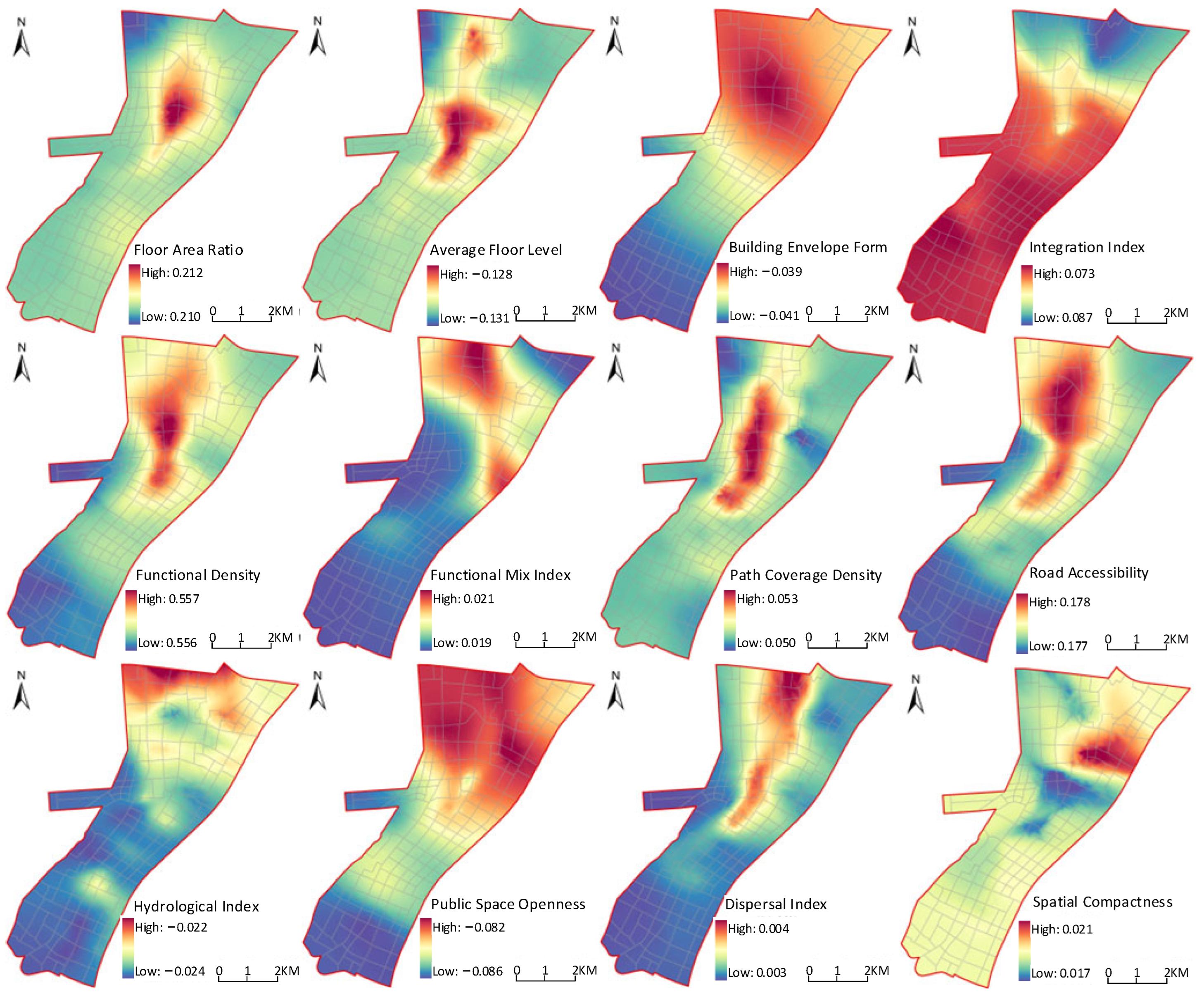
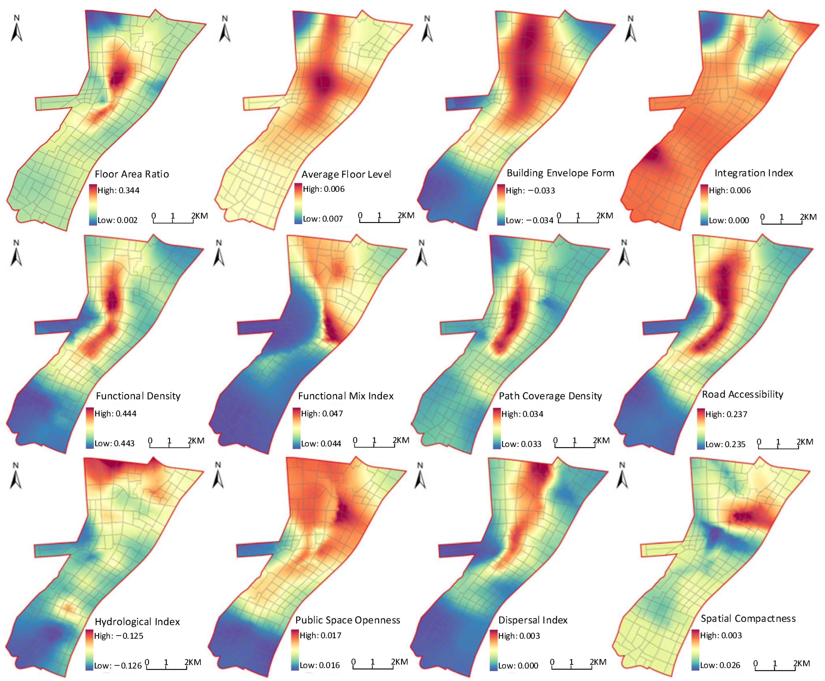
4.2.2. Vitality in Relation to the Built Environment
5. Discussion
5.1. The Influencing Factors of Coastal Spatial Vitality Exhibit Differentiation
5.2. Design-Guided Strategies for Block Spaces
5.3. Mechanisms for the Construction and Development of Coastal Cities
6. Conclusions
Author Contributions
Funding
Data Availability Statement
Acknowledgments
Conflicts of Interest
Appendix A

| Major Categories of Influencing Factors | Number | Category | Formulas | Interpretation |
|---|---|---|---|---|
| Block morphology | X1 | Floor area ratio | represents the site area. | It refers to the ratio of a building’s total floor area to the area of the land it occupies. |
| X2 | Average floor level | represents the site area. | It describes the vertical stacking of building spaces within a plot, serving as a way to reflect the degree of spatial aggregation of buildings. | |
| X3 | Building envelope form | The combinations of buildings within the block can be roughly divided into free-style combinations, row-style combinations, cluster-style combinations, courtyard-style combinations, detached combinations, and mixed combinations. | Architectural spatial composition includes various types of individual buildings, group buildings, and their enclosed spaces. | |
| X4 | Integration index | represents the spatial area of the block. | The block shape integration degree reflects the regularity of an individual block’s form. The smaller the block shape integration degree, the more uniform and regular the block’s texture tends to be. | |
| X5 | Form fragmentation index | represents the standard deviation of building areas (m2). | This measure reflects the spatial form generated within the block, assessing the morphological characteristics exhibited by the overall layout of buildings within the block. | |
| Facility function | X6 | Functional density | represents the number of POIs; and Ai represents the area of the block. | The density measurement of points of interest (POIs) within the block. |
| X7 | Functional mix index | refers to the proportion of the j-th type of function within block i; and M refers to the number of functional categories within the current block. | The proportion of points of interest (POI) data within the block. | |
| Road network structure | X8 | Path coverage density | represents the perimeter of block i. | The ratio of the total length of pathways within a block to the perimeter of the block, which can evaluate the richness of the block’s road network structure and road variations. |
| X9 | Road accessibility | AI stands for the road accessibility; NC represents the total number of nodes (intersections) of roads; and TD represents the total depth value of roads. | Quantitative analysis of the convenience of residents reaching the block. | |
| Architectural features | X10 | Hydrological index | represents the spatial linear distance between block unit i and the surrounding water system w. | The nearest distance from spatial units to adjacent water bodies serves as an indicator to measure waterfront accessibility. |
| X11 | Public space openness | is the ground space index. | The size of public spaces within the block. | |
| X12 | Dispersal index | is the standard deviation of heights; and H is the average height of buildings within the block. | The difference between the average and maximum building heights within the plot. | |
| X13 | Spatial compactness | C stands for spatial compactness; A is the total building footprint area within the block; and P is the perimeter of the total building footprints within the block. | The geometric distribution of total buildings within the block, analyzing the compactness of the block. |
| Variable | Tourism Off-Peak Season | Tourism Peak Season | ||||||||
|---|---|---|---|---|---|---|---|---|---|---|
| Mean | Standard Deviation | Min. | Median | Max. | Mean | Standard Deviation | Min. | Median | Max. | |
| X1 (floor area ratio) | 0.211 | 0.001 | 0.21 | 0.211 | 0.212 | 0.346 | 0.001 | 0.344 | 0.346 | 0.348 |
| X2 (average floor level) | −0.13 | 0.001 | −0.131 | −0.13 | −0.128 | 0.006 | 0 | 0.006 | 0.006 | 0.007 |
| X3 (building envelope form) | −0.04 | 0 | −0.041 | −0.04 | −0.039 | −0.033 | 0 | −0.034 | −0.033 | −0.033 |
| X4 (integration index) | 0.07 | 0.001 | 0.067 | 0.07 | 0.073 | 0.003 | 0.002 | 0 | 0.003 | 0.006 |
| X5 (fragmentation index) | 0.01 | 0 | 0.01 | 0.01 | 0.011 | 0.005 | 0.001 | 0.003 | 0.005 | 0.006 |
| X6 (functional density) | 0.557 | 0 | 0.556 | 0.557 | 0.557 | 0.444 | 0 | 0.443 | 0.444 | 0.444 |
| X7 (functional mix index) | 0.02 | 0.001 | 0.019 | 0.02 | 0.021 | 0.045 | 0.001 | 0.044 | 0.045 | 0.047 |
| X8 (path coverage density) | 0.052 | 0.001 | 0.05 | 0.052 | 0.053 | 0.033 | 0 | 0.033 | 0.033 | 0.034 |
| X9 (road accessibility) | 0.177 | 0.001 | 0.177 | 0.177 | 0.178 | 0.236 | 0 | 0.235 | 0.236 | 0.237 |
| X10 (hydrological index) | −0.023 | 0.001 | −0.024 | −0.023 | −0.022 | −0.126 | 0 | −0.126 | −0.126 | −0.125 |
| X11 (public space openness) | −0.084 | 0.001 | −0.086 | −0.084 | −0.082 | 0.017 | 0 | 0.016 | 0.017 | 0.017 |
| X12 (dispersal index) | 0.004 | 0 | 0.003 | 0.004 | 0.004 | 0.001 | 0.001 | 0 | 0.001 | 0.003 |
| X13 (spatial compactness) | 0.019 | 0.001 | 0.017 | 0.019 | 0.021 | 0.03 | 0.002 | 0.026 | 0.029 | 0.033 |
| Performance statistics | ||||||||||
| R-squared | 0.73 | 0.744 | ||||||||
| Adjusted R-squared | 0.702 | 0.718 | ||||||||
| AICc | 289.723 | 279.343 | ||||||||
| BIC | 337.869 | 325.355 | ||||||||
| Number of observations | 165 | |||||||||
| Variable | Harbor District | Tourism-Driven District | ||||||||
|---|---|---|---|---|---|---|---|---|---|---|
| Mean | Standard Deviation | Min. | Median | Max. | Mean | Standard Deviation | Min. | Median | Max. | |
| X1 (floor area ratio) | 0.29 | 0 | 0.289 | 0.29 | 0.29 | 0.356 | 0.01 | 0.339 | 0.356 | 0.375 |
| X2 (average floor level) | −0.125 | 0.001 | −0.127 | −0.125 | −0.124 | −0.027 | 0.001 | −0.029 | −0.027 | −0.026 |
| X3 (building envelope form) | −0.058 | 0 | −0.059 | −0.058 | −0.057 | −0.024 | 0 | −0.024 | −0.024 | −0.024 |
| X4 (integration index) | 0.146 | 0 | 0.145 | 0.146 | 0.147 | −0.046 | 0 | −0.047 | −0.046 | −0.046 |
| X5 (fragmentation index) | −0.066 | 0 | −0.066 | −0.066 | −0.065 | 0.036 | 0.001 | 0.035 | 0.036 | 0.038 |
| X6 (functional density) | 0.534 | 0 | 0.534 | 0.534 | 0.534 | 0.42 | 0 | 0.42 | 0.42 | 0.421 |
| X7 (functional mix index) | 0.148 | 0 | 0.148 | 0.148 | 0.149 | −0.046 | 0 | −0.046 | −0.046 | −0.045 |
| X8 (path coverage density) | 0.025 | 0.001 | 0.023 | 0.025 | 0.026 | 0.09 | 0 | 0.089 | 0.09 | 0.09 |
| X9 (road accessibility) | 0.27 | 0 | 0.27 | 0.27 | 0.271 | 0.072 | 0 | 0.072 | 0.072 | 0.073 |
| X10 (hydrological index) | −0.154 | 0 | −0.155 | −0.154 | −0.153 | −0.08 | 0 | −0.08 | −0.08 | −0.079 |
| X11 (public space openness) | 0.007 | 0 | 0.007 | 0.007 | 0.007 | 0.017 | 0.001 | 0.016 | 0.018 | 0.019 |
| X12 (dispersal index) | −0.006 | 0 | −0.007 | −0.006 | −0.005 | 0.054 | 0 | 0.054 | 0.054 | 0.054 |
| X13 (spatial compactness) | −0.122 | 0 | −0.122 | −0.122 | −0.122 | 0.109 | 0.001 | 0.107 | 0.109 | 0.11 |
| Performance statistics | ||||||||||
| R-squared | 0.745 | 0.743 | ||||||||
| Adjusted R-squared | 0.685 | 0.691 | ||||||||
| AICc | 150.292 | 170.109 | ||||||||
| BIC | 177.370 | 201.761 | ||||||||
| Number of observations | 76 | 89 | ||||||||
References
- Liu, G.; Li, J.; Nie, P. Tracking the history of urban expansion in Guangzhou (China) during 1665–2017: Evidence from historical maps and remote sensing images. Land Use Policy 2022, 112, 105773. [Google Scholar] [CrossRef]
- Eisemon, T.O. Benefiting from Basic Education, School Quality and Functional Literacy in Kenya; Elsevier: Amsterdam, The Netherlands, 2014; Volume 2, pp. 150–174. [Google Scholar]
- Yuko, E. How the Industrial Revolution Fueled the Growth of Cities. 2021. Available online: https://www.history.com/news/industrial-revolution-cities (accessed on 10 May 2023).
- Yang, L.; Wei, C.; Jiang, X.; Ye, Q.; Tatano, H. The new urbanization policy in China: Which way forward? Habitat Int. 2015, 47, 279–284. [Google Scholar]
- Chen, M.; Ye, C.; Lu, D.; Sui, Y.; Guo, S. Cognition and construction of the theoretical connotations of new urbanization with Chinese characteristics. J. Geogr. Sci. 2019, 29, 1681–1698. [Google Scholar] [CrossRef]
- Chen, M.; Liu, W.; Tao, X. Evolution and assessment on China’s urbanization 1960–2010: Under-urbanization or over-urbanization? Habitat Int. 2013, 38, 25–33. [Google Scholar] [CrossRef]
- Guan, X.; Wei, H.; Lu, S.; Dai, Q.; Su, H. Assessment on the urbanization strategy in China: Achievements, challenges and reflections. Habitat Int. 2018, 71, 97–109. [Google Scholar] [CrossRef]
- Yang, L.; Luo, X.; Ding, Z.; Liu, X.; Gu, Z. Restructuring for growth in development zones, China: A systematic literature and policy review (1984–2022). Land 2022, 11, 972. [Google Scholar] [CrossRef]
- Gao, S.; Wang, S.; Sun, D. Development zones and their surrounding host cities in China: Isolation and mutually beneficial interactions. Land 2021, 11, 20. [Google Scholar] [CrossRef]
- Shen, Y.; Zhang, X.; Zhu, H.; Yin, Z.; Drianda, R.P. Living in a Chinese Industrial New Town: A Case Study of Chenglingji New Port Area. Land 2023, 12, 790. [Google Scholar] [CrossRef]
- Long, H.; Liu, Y.; Hou, X.; Li, T.; Li, Y. Effects of land use transitions due to rapid urbanization on ecosystem services: Implications for urban planning in the new developing area of China. Habitat Int. 2014, 44, 536–544. [Google Scholar] [CrossRef]
- Hu, Y.; Wang, Z.; Deng, T. Expansion in the shrinking cities: Does place-based policy help to curb urban shrinkage in China? Cities 2021, 113, 103188. [Google Scholar] [CrossRef]
- Long, Y.; Gao, S. Shrinking cities in China: The overall profile and paradox in planning. In Shrinking Cities in China: The Overall Profile and Paradox in Planning; Springer: Berlin/Heidelberg, Germany, 2019; pp. 3–21. [Google Scholar]
- Zhang, Y.; Fu, Y.; Kong, X.; Zhang, F. Prefecture-level city shrinkage on the regional dimension in China: Spatiotemporal change and internal relations. Sustain. Cities Soc. 2019, 47, 101490. [Google Scholar] [CrossRef]
- Taubenböck, H.; Shi, L.; Leichtle, T.; Du, S.; Wurm, M. The ‘ghost city’phenomenon in China: Mapping and categorization at intra-urban scale. In Proceedings of the 2023 Joint Urban Remote Sensing Event (JURSE), Heraklion, Greece, 17–19 May 2023; IEEE: Piscataway, NJ, USA, 2023; pp. 1–4. [Google Scholar]
- Dong, L.; Du, R.; Kahn, M.; Ratti, C.; Zheng, S. “Ghost cities” versus boom towns: Do China’s high-speed rail new towns thrive? Reg. Sci. Urban Econ. 2021, 89, 103682. [Google Scholar] [CrossRef]
- Shi, L.; Wurm, M.; Huang, X.; Zhong, T.; Leichtle, T.; Taubenböck, H. Urbanization that hides in the dark—Spotting China’s “ghost neighborhoods” from space. Landsc. Urban Plan. 2020, 200, 103822. [Google Scholar] [CrossRef]
- Mouratidis, K. Urban planning and quality of life: A review of pathways linking the built environment to subjective well-being. Cities 2021, 115, 103229. [Google Scholar] [CrossRef]
- Sheikh, W.T.; van Ameijde, J. Promoting livability through urban planning: A comprehensive framework based on the “theory of human needs”. Cities 2022, 131, 103972. [Google Scholar] [CrossRef]
- Rydin, Y.; Bleahu, A.; Davies, M.; Dávila, J.D.; Friel, S.; De Grandis, G.; Groce, N.; CHallal, P.; Hamilton, I.; Howden-Chapman, P.; et al. Shaping cities for health: Complexity and the planning of urban environments in the 21st century. Lancet 2012, 379, 2079–2108. [Google Scholar] [CrossRef]
- Paköz, M.Z.; Işık, M. Rethinking urban density, vitality and healthy environment in the post-pandemic city: The case of Istanbul. Cities 2022, 124, 103598. [Google Scholar] [CrossRef]
- Pittman, S.J.; Rodwell, L.D.; Shellock, R.J.; Williams, M.; Attrill, M.J.; Bedford, J.; Curry, K.; Fletcher, S.; Gall, S.C.; Lowther, J.; et al. Marine parks for coastal cities: A concept for enhanced community well-being, prosperity and sustainable city living. Mar. Policy 2019, 103, 160–171. [Google Scholar] [CrossRef]
- Zheng, Z.; Wu, Z.; Chen, Y.; Yang, Z.; Marinello, F. Exploration of eco-environment and urbanization changes in coastal zones: A case study in China over the past 20 years. Ecol. Indic. 2020, 119, 106847. [Google Scholar] [CrossRef]
- Liu, D.; Xing, W. Analysis of China’s coastal zone management reform based on land-sea integration. Mar. Econ. Manag. 2019, 2, 39–49. [Google Scholar] [CrossRef]
- Yılmaz, M.; Terzi, F. Measuring the patterns of urban spatial growth of coastal cities in developing countries by geospatial metrics. Land Use Policy 2021, 107, 105487. [Google Scholar] [CrossRef]
- Zhang, H.; Chen, S. Overview of research on marine resources and economic development. Mar. Econ. Manag. 2022, 5, 69–83. [Google Scholar] [CrossRef]
- Ding, G.; Guo, J.; Pueppke, S.G.; Ou, M.; Ou, W.; Tao, Y. Has urban form become homogenizing? Evidence from cities in China. Ecol. Indic. 2022, 144, 109494. [Google Scholar] [CrossRef]
- Elmqvist, T.; Andersson, E.; Frantzeskaki, N.; McPhearson, T.; Olsson, P.; Gaffney, O.; Takeuchi, K.; Folke, C. Sustainability and resilience for transformation in the urban century. Nat. Sustain. 2019, 2, 267–273. [Google Scholar] [CrossRef]
- Mouratidis, K. Built environment and social well-being: How does urban form affect social life and personal relationships? Cities 2018, 74, 7–20. [Google Scholar] [CrossRef]
- Liu, G.; Lei, J.; Qin, H.; Niu, J.; Chen, J.; Lu, J.; Han, G. Impact of environmental comfort on urban vitality in small and medium-sized cities: A case study of Wuxi County in Chongqing, China. Front. Public Health 2023, 11, 1131630. [Google Scholar] [CrossRef]
- Nathansohn, R.; Lahat, L. From urban vitality to urban vitalisation: Trust, distrust, and citizenship regimes in a Smart City initiative. Cities 2022, 131, 103969. [Google Scholar] [CrossRef]
- Zhang, F.; Liu, Q.; Zhou, X. Vitality evaluation of public spaces in historical and cultural blocks based on multi-source data, a case study of Suzhou Changmen. Sustainability 2022, 14, 14040. [Google Scholar] [CrossRef]
- Liu, S.; Zhang, L.; Long, Y. Urban vitality area identification and pattern analysis from the perspective of time and space fusion. Sustainability 2019, 11, 4032. [Google Scholar] [CrossRef]
- Lan, F.; Gong, X.; Da, H.; Wen, H. How do population inflow and social infrastructure affect urban vitality? Evidence from 35 large-and medium-sized cities in China. Cities 2020, 100, 102454. [Google Scholar] [CrossRef]
- Ye, Y.; Li, D.; Liu, X. How block density and typology affect urban vitality: An exploratory analysis in Shenzhen, China. Urban Geogr. 2018, 39, 631–652. [Google Scholar] [CrossRef]
- Xia, C.; Yeh, A.G.O.; Zhang, A. Analyzing spatial relationships between urban land use intensity and urban vitality at street block level: A case study of five Chinese megacities. Landsc. Urban Plan. 2020, 193, 103669. [Google Scholar] [CrossRef]
- Wang, F.; Liu, Z.; Shang, S.; Qin, Y.; Wu, B. Vitality continuation or over-commercialization? Spatial structure characteristics of commercial services and population agglomeration in historic and cultural areas. Tour. Econ. 2019, 25, 1302–1326. [Google Scholar] [CrossRef]
- Zikirya, B.; He, X.; Li, M.; Zhou, C. Urban food takeaway vitality: A new technique to assess urban vitality. Int. J. Environ. Res. Public Health 2021, 18, 3578. [Google Scholar] [CrossRef] [PubMed]
- He, Q.; He, W.; Song, Y.; Wu, J.; Yin, C.; Mou, Y. The impact of urban growth patterns on urban vitality in newly built-up areas based on an association rules analysis using geographical ‘big data’. Land Use Policy 2018, 78, 726–738. [Google Scholar] [CrossRef]
- Liu, S.; Ge, J.; Ye, X.; Wu, C.; Bai, M. Urban vitality assessment at the neighborhood scale with geo-data: A review toward implementation. J. Geogr. Sci. 2023, 33, 1482–1504. [Google Scholar] [CrossRef]
- Still, B.; Simmonds, D. Parking restraint policy and urban vitality. Transp. Rev. 2000, 20, 291–316. [Google Scholar] [CrossRef]
- Zhu, J.; Lu, H.; Zheng, T.; Rong, Y.; Wang, C.; Zhang, W.; Yan, Y.; Tang, L. Vitality of urban parks and its influencing factors from the perspective of recreational service supply, demand, and spatial links. Int. J. Environ. Res. Public Health 2020, 17, 1615. [Google Scholar] [CrossRef] [PubMed]
- Fan, Z.; Duan, J.; Luo, M.; Zhan, H.; Liu, M.; Peng, W. How did built environment affect urban vitality in urban waterfronts? A case study in Nanjing reach of Yangtze River. ISPRS Int. J. Geo-Inf. 2021, 10, 611. [Google Scholar] [CrossRef]
- Liu, S.; Lai, S.Q.; Liu, C.; Jiang, L. What influenced the vitality of the waterfront open space? A case study of Huangpu River in Shanghai, China. Cities 2021, 114, 103197. [Google Scholar] [CrossRef]
- Yin, Y.; Shao, Y.; Lu, H.; Han, Y. Environmental drivers of the vital urban coastal zones: An explorative case study based on the data-driven multi-method approach. Front. Ecol. Evol. 2022, 10, 962299. [Google Scholar] [CrossRef]
- Benson, E. Rivers as urban landscapes: Renaissance of the waterfront. Water Sci. Technol. 2002, 45, 65–70. [Google Scholar] [CrossRef] [PubMed]
- Lee, P.T.W.; Wu, J.Z.; Hu, K.C.; Flynn, M. Applying analytic network process (ANP) to rank critical success factors of waterfront redevelopment. Int. J. Shipp. Transp. Logist. 2013, 5, 390–411. [Google Scholar] [CrossRef]
- Üzümcüoğlu, D.; Polay, M. Urban waterfront development, through the lens of the Kyrenia waterfront case study. Sustainability 2022, 14, 9469. [Google Scholar] [CrossRef]
- Chang, T.C.; Huang, S.; Savage, V.R. On the waterfront: Globalization and urbanization in Singapore. Urban Geogr. 2004, 25, 413–436. [Google Scholar] [CrossRef]
- Chen, W.; Wu, A.N.; Biljecki, F. Classification of urban morphology with deep learning: Application on urban vitality. Comput. Environ. Urban Syst. 2021, 90, 101706. [Google Scholar] [CrossRef]
- Dong, Y.H.; Peng, F.L.; Guo, T.F. Quantitative assessment method on urban vitality of metro-led underground space based on multi-source data: A case study of Shanghai Inner Ring area. Tunn. Undergr. Space Technol. 2021, 116, 104108. [Google Scholar] [CrossRef]
- Sairinen, R.; Kumpulainen, S. Assessing social impacts in urban waterfront regeneration. Environ. Impact Assess. Rev. 2006, 26, 120–135. [Google Scholar] [CrossRef]
- Hein, C.; van de Laar, P.T. The separation of ports from cities: The case of Rotterdam. In European Port Cities in Transition: Moving towards More Sustainable Sea Transport Hubs; Springer: Berlin/Heidelberg, Germany, 2020; pp. 265–286. [Google Scholar]
- Giles-Corti, B.; Broomhall, M.H.; Knuiman, M.; Collins, C.; Douglas, K.; Ng, K.; Langea Donovan, R.J. Increasing walking: How important is distance to, attractiveness, and size of public open space? Am. J. Prev. Med. 2005, 28, 169–176. [Google Scholar] [CrossRef]
- Li, X.; Li, Y.; Jia, T.; Zhou, L.; Hijazi, I.H. The six dimensions of built environment on urban vitality: Fusion evidence from multi-source data. Cities 2022, 121, 103482. [Google Scholar] [CrossRef]
- Guo, X.; Yang, Y.; Cheng, Z.; Wu, Q.; Li, C.; Lo, T.; Chen, F. Spatial social interaction: An explanatory framework of urban space vitality and its preliminary verification. Cities 2022, 121, 103487. [Google Scholar] [CrossRef]
- Woo, S.W.; Omran, A.; Lee, C.L.; Hanafi, M.H. The impacts of the waterfront development in Iskandar Malaysia. Environ. Dev. Sustain. 2017, 19, 1293–1306. [Google Scholar] [CrossRef]
- Wang, Y.; Dewancker, B.J.; Qi, Q. Citizens’ preferences and attitudes towards urban waterfront spaces: A case study of Qiantang riverside development. Environ. Sci. Pollut. Res. 2020, 27, 45787–45801. [Google Scholar] [CrossRef] [PubMed]
- Shangi, Z.A.D.; Hasan, M.T.; Ahmad, M.I. Rethinking Urban Waterfront as a Potential Public Open Space: Interpretative Framework of Surma Waterfront. Archit. Res. 2020, 10, 69–74. [Google Scholar]
- Wu, D.; Niu, Y.; Sun, Z. Quantitative Research on the Quality of Street Space in Coastal Cities. J. Coast. Res. 2020, 106, 423–426. [Google Scholar] [CrossRef]
- Lyu, G.; Angkawisittpan, N.; Fu, X.; Sonasang, S. Enhancing Urban Vitality through Big Data: A Case Study of Yinchuan City Using GWR and GBDT Models. 2023. Available online: https://www.researchsquare.com/article/rs-3590148/v1 (accessed on 10 May 2023).
- Wangbao, L. Spatial impact of the built environment on street vitality: A case study of the Tianhe District, Guangzhou. Front. Environ. Sci. 2022, 10, 966562. [Google Scholar] [CrossRef]
- Qin, L.; Zong, W.; Peng, K.; Zhang, R. Assessing Spatial Heterogeneity in Urban Park Vitality for a Sustainable Built Environment: A Case Study of Changsha. Land 2024, 13, 480. [Google Scholar] [CrossRef]
- Sternhao, H.; Yang, X.; Yue, J. Analysis of urban road cycling flow based on multi-scale geographically weighted regression model. J. Tsinghua Univ. 2022, 62, 1132–1141. [Google Scholar]
- Chen, Z.; Deng, Z. Study on the relationship between neighborhood morphology and heat island intensity in the main urban area of Guangzhou based on multi-scale geographically weighted regression. Intell. Build. Smart City 2021, 5. [Google Scholar]
- Yang, L.; Wei, C.; Jiang, X.; Ye, Q.; Tatano, H. Estimating the economic effects of the early Covid-19 emergency response in cities using Intracity travel intensity data. Int. J. Disaster Risk Sci. 2022, 13, 125–138. [Google Scholar] [CrossRef]
- Statistical Bulletin of National Economic and Social Development of Mackerel Circle District, Yingkou City, 2020. Available online: http://www.ykdz.gov.cn/govxxgk/kfq/2021-06-24/f76a997e-ceb9-484a-97f7-361de438c7ee.html (accessed on 10 May 2023).
- Saito, A. Global city formation in a capitalist developmental state: Tokyo and the waterfront sub-centre project. Urban Stud. 2003, 40, 283–308. [Google Scholar] [CrossRef]
- Edwards, D.; Griffin, T.; Hayllar, B. Darling Harbour: Looking back and moving forward. In City Spaces—Tourist Places; Routledge: London, UK, 2010; pp. 275–294. [Google Scholar]
- Stevens, Q. Tracing the Shifting Waterfront. In Activating Urban Waterfronts; Routledge: London, UK, 2020; pp. 72–91. [Google Scholar]
- Gadomska, W. Modern park as a result of urban space recycling—A review of New York City’s developments. Tech. Trans. 2018, 10, 5–21. [Google Scholar]
- Chen, Y. New approaches for calculating Moran’s index of spatial autocorrelation. PLoS ONE 2013, 8, e68336. [Google Scholar] [CrossRef] [PubMed]
- Pohlmann, J.T.; Dennis, W.L. A comparison of ordinary least squares and logistic regression (1). Ohio J. Sci. 2003, 103, 118–126. [Google Scholar]
- Thapa, R.B.; Ronald, C.E. Geographically weighted regression in geospatial analysis. In Progress in Geospatial Analysis; Springer: Tokyo, Japan, 2012; pp. 85–96. [Google Scholar]
- Erysheva, E.; Moor, V. Visual Identity of Seaside City’s Cultural Landscape. IOP Conf. Ser. Mater. Sci. Eng. 2021, 3, 1079. [Google Scholar] [CrossRef]
- World Population Prospects 2022: Summary of Results. Available online: https://www.un.org/development/desa/pd/content/World-Population-Prospects-2022 (accessed on 10 May 2023).
- Li, Y.; Huang, C. The spatio-temporal dynamics of the green space and landscape in rapidly urbanizing Shanghai. CABI Digit. Libr. 2017, 10, 87–93. [Google Scholar]
- Fenton, P. Port-city redevelopment and sustainable development. In European Port Cities in Transition: Moving towards More Sustainable Sea Transport Hubs; Springer: Berlin/Heidelberg, Germany, 2020; Volume 3, pp. 19–36. [Google Scholar]
- Yang, Y.; Ma, Y.; Jiao, H. Exploring the correlation between block vitality and block environment based on multisource big data: Taking Wuhan City as an example. Land 2021, 10, 984. [Google Scholar] [CrossRef]
- Zhao, P.; Wan, J. Examining the effects of neighbourhood design on walking in growing megacity. Transp. Res. Part D Transp. Environ. 2020, 86, 102417. [Google Scholar] [CrossRef]
- Chng, L.C.; Chou, L.M.; Huang, D. Environmental performance indicators for the urban coastal environment of Singapore. Reg. Stud. Mar. Sci. 2022, 49, 102101. [Google Scholar] [CrossRef]
- Qian, W.; Zhao, Y.; Li, X. Construction of ecological security pattern in coastal urban areas: A case study in Qingdao, China. Ecol. Indic. 2023, 154, 110754. [Google Scholar] [CrossRef]
- Zhou, L.; Kong, X.; Shen, G.; Li, Y.; Zhu, H.; Chen, T.; Yan, Y.; Liu, Y. Spatial-temporal impacts of landscape metrics and uses of land reclamation on coastal water conditions: The case of Macao. Ecol. Indic. 2023, 154, 110518. [Google Scholar] [CrossRef]
- Gan, X.; Huang, L.; Wang, H.; Mou, Y.; Wang, D.; Hu, A. Optimal block size for improving urban vitality: An exploratory analysis with multiple vitality indicators. J. Urban Plan. Dev. 2021, 147, 04021027. [Google Scholar] [CrossRef]
- Wang, J.; Zheng, L.; Liu, H.; Xu, B.; Zou, Z. The effects of habitat network construction and urban block unit structure on biodiversity in semiarid green spaces. Environ. Monit. Assess. 2020, 192, 1–23. [Google Scholar] [CrossRef] [PubMed]
- Wang, X.; Song, Y.; Tang, P. Generative urban design using shape grammar and block morphological analysis. Front. Archit. Res. 2020, 9, 914–924. [Google Scholar] [CrossRef]
- van Nes, A.; Yamu, C.; van Nes, A.; Yamu, C. Private and public space: Analysing spatial relationships between buildings and streets. In Introduction to Space Syntax in Urban Studies; Springer: Berlin/Heidelberg, Germany, 2021; Volume 23, pp. 113–131. [Google Scholar]
- Wang, Y.; Peng, Z.; Chen, Q. The choice of residential layout in urban China: A comparison of transportation and land use in Changsha (China) and Leeds (UK). Habitat Int. 2018, 75, 50–58. [Google Scholar] [CrossRef]
- Shakibamanesh, A.; Ebrahimi, B. Toward practical criteria for analyzing and designing urban blocks. Sustain. Urban Plan. Des. 2020, 12, 185. [Google Scholar]
- Mega, V.P.; Mega, V.P. Sustainable Regeneration of Coastal Cities. Conscious Coastal Cities: Sustainability. Blue Green Growth Politics Imagin. 2016, 34, 223–252. [Google Scholar]
- Zhu, X. Optimization Design of Public Space Structure in Coastal Cities Based on Interactive Design. J. Coast. Res. 2020, 104, 751–755. [Google Scholar] [CrossRef]
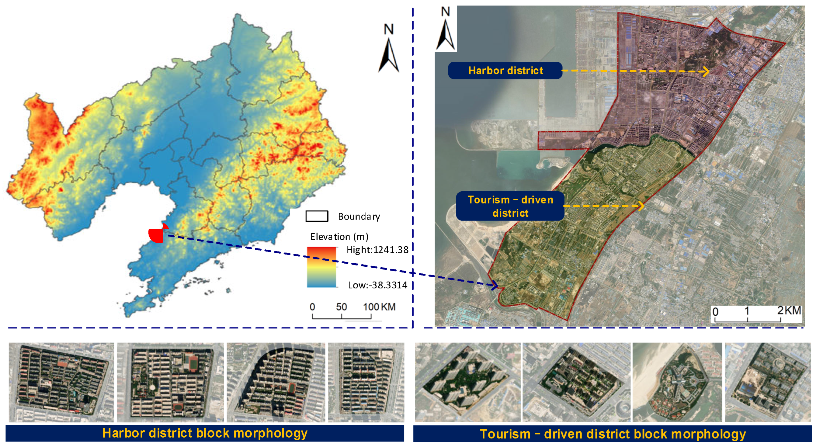


| Different Zones | Total Area | Built-Up Area | Proportion of Green Area |
|---|---|---|---|
| Harbor district block morphology | 21.16 km2 | 91.81% | 7.85% |
| Tourism-driven district block morphology | 20.10 km2 | 41.55% | 6.93% |
| Data | Format | Attributes | Source |
|---|---|---|---|
| Baidu heat map | .tif | Location, intensity value, and timestamp | China Baidu Map (https://map.baidu.com/ (accessed on 1 July 2019, 12 July 2019, 13 July 2019, 1 November 2019, 8 November 2019 and 9 November 2019)) |
| Bayuquan administrative boundaries and water systems | .shp | Area and name | China Basic Geographic Information System 1:2 million data |
| Road | .shp | Width and length | Open Street Map (https://openmaptiles.org/ (accessed on 10 May 2019)) |
| POI | .xlsx | Name, type, latitude, and longitude | China Baidu Map (https://map.baidu.com/ (accessed on 10 May 2019)) |
| Building | .shp | Width, length, and grade of roads | Google Earth (https://www.google.cn/ (accessed on 10 May 2019)) |
| Satellite remote-sensing images | .tif | Time and spectral information | Google Earth (https://www.google.cn/ (accessed on 10 May 2019)) |
| Off-Peak Season | Peak Season | Annual Average | |
|---|---|---|---|
| Moran’s I | 0.524878 | 0.529371 | 0.516968 |
| Z-value | 10.703993 | 10.762103 | 10.709803 |
| p-value | 0.0001 | 0.0001 | 0.0001 |
| Variables | Tourism Off-Peak Season | Tourism Peak Season | VIF | ||||||
|---|---|---|---|---|---|---|---|---|---|
| Coefficient | Standard Deviation | T-Value | Robust | Coefficient | Standard Deviation | T-Value | Robust | ||
| X1 | 1.700 | 0.890 | 1.910 | 0.003 * | 3.217 | 0.990 | 3.248 | 0.008 * | 6.511 |
| X2 | −0.165 | 0.115 | −1.434 | 0.035 * | 0.008 | 0.128 | 0.064 | 0.024 * | 4.351 |
| X3 | 0.000 | 0.000 | −0.778 | 0.023 * | 0.000 | 0.000 | 0.678 | 0.014 * | 1.388 |
| X4 | 2.527 | 2.956 | 0.855 | 0.023 * | 0.142 | 3.289 | 0.043 | 0.045 * | 3.572 |
| X5 | 0.000 | 0.000 | 0.163 | 0.080 | 0.000 | 0.000 | 0.073 | 0.094 | 1.982 |
| X6 | 1.841 | 0.210 | 8.781 | 0.000 * | 1.696 | 0.233 | 7.273 | 0.000 * | 2.145 |
| X7 | 0.436 | 1.059 | 0.411 | 0.034 * | 1.129 | 1.178 | 0.959 | 0.024 * | 1.275 |
| X8 | 0.478 | 0.662 | 0.722 | 0.017 * | 0.363 | 0.737 | 0.493 | 0.016 * | 2.795 |
| X9 | 0.205 | 0.079 | 2.587 | 0.011 * | 0.316 | 0.088 | 3.571 | 0.001 * | 2.509 |
| X10 | 0.000 | 0.000 | −0.447 | 0.015 * | 0.001 | 0.000 | 2.483 | 0.006 * | 1.472 |
| X11 | −1.548 | 1.662 | −0.931 | 0.030 * | 0.360 | 1.849 | 0.195 | 0.033 * | 4.273 |
| X12 | 0.060 | 1.087 | 0.055 | 0.047 * | 0.026 | 1.209 | 0.022 | 0.017 * | 2.225 |
| X13 | 0.629 | 3.598 | 0.175 | 0.020 * | 1.134 | 4.004 | 0.283 | 0.016 * | 6.080 |
| Performance statistics | |||||||||
| R-squared | 0.717 | 0.738 | |||||||
| Adjusted R-squared | 0.692 | 0.715 | |||||||
| AIC | 888.701 | 923.972 | |||||||
| Koenker (BP) | 0.000831 * | 0.017201 * | |||||||
| Variable | Harbor District | Tourism-Driven District | ||||||||
|---|---|---|---|---|---|---|---|---|---|---|
| Coefficient | Standard Deviation | T-Value | Robust | VIF | Coefficient | Standard Deviation | T-Value | Robust | VIF | |
| X1 | 3.408 | 2.066 | 2.066 | 0.002 * | 7.394 | 2.244 | 0.952 | 2.357 | 0.001 * | 6.836 |
| X2 | −0.329 | 0.425 | 0.425 | 0.037 * | 6.430 | −0.033 | 0.121 | −0.273 | 0.006 * | 5.301 |
| X3 | 0.000 | 0.000 | 0.000 | 0.049 * | 2.043 | 0.000 | 0.000 | −0.357 | 0.002 * | 1.379 |
| X4 | 6.527 | 6.589 | 6.589 | 0.010 * | 5.319 | −1.811 | 3.669 | −0.494 | 0.016 * | 4.218 |
| X5 | −0.001 | 0.002 | 0.002 | 0.0758 | 4.016 | 0.000 | 0.000 | 0.421 | 0.060 | 2.462 |
| X6 | 1.941 | 0.353 | 0.353 | 0.000 * | 2.293 | 1.406 | 0.272 | 5.167 | 0.000 * | 1.911 |
| X7 | 4.305 | 2.405 | 2.405 | 0.008 * | 1.632 | −0.725 | 1.148 | −0.632 | 0.003 * | 1.304 |
| X8 | 0.221 | 1.235 | 1.235 | 0.005 * | 4.364 | 1.024 | 1.012 | 1.012 | 0.003 * | 2.526 |
| X9 | 0.289 | 0.155 | 0.155 | 0.041 * | 5.155 | 0.135 | 0.162 | 0.833 | 0.004 * | 2.248 |
| X10 | −0.001 | 0.000 | 0.000 | 0.046 * | 1.831 | −0.001 | 0.000 | −1.231 | 0.002 * | 1.741 |
| X11 | 0.150 | 3.646 | 3.646 | 0.009 * | 3.435 | 0.186 | 1.990 | 0.093 | 0.021 * | 6.035 |
| X12 | −0.140 | 2.053 | 2.053 | 0.009 * | 1.868 | 0.648 | 1.321 | 0.491 | 0.005 * | 2.694 |
| X13 | −5.067 | 6.724 | 6.724 | 0.027 * | 6.390 | 3.937 | 4.773 | 0.825 | 0.035 * | 6.512 |
| Performance statistics | ||||||||||
| R-squared | 0.744 | 0.735 | ||||||||
| Adjusted R-squared | 0.685 | 0.689 | ||||||||
| AIC | 448.766 | 465.195 | ||||||||
| Koenker(BP) | 0.173 | 0.018321 * | ||||||||
| Different Districts | Main Factors Affecting Spatial Vitality |
|---|---|
| Harbor district | Integration index, functional density, functional mix index, and path coverage density |
| Tourism-driven district | Hydrological index, public space openness, dispersal index, and spatial compactness |
| Layout Patterns | Free Form | Linear Form | Radiolucent Form | Branch Form | Grid Form |
|---|---|---|---|---|---|
| Tree-shaped |  |  | 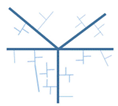 |  | 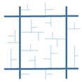 |
| Grid-shaped |  |  |  |  |  |
Disclaimer/Publisher’s Note: The statements, opinions and data contained in all publications are solely those of the individual author(s) and contributor(s) and not of MDPI and/or the editor(s). MDPI and/or the editor(s) disclaim responsibility for any injury to people or property resulting from any ideas, methods, instructions or products referred to in the content. |
© 2024 by the authors. Licensee MDPI, Basel, Switzerland. This article is an open access article distributed under the terms and conditions of the Creative Commons Attribution (CC BY) license (https://creativecommons.org/licenses/by/4.0/).
Share and Cite
Hu, C.; Xu, L.; Cai, X.; Tian, D.; Zhuang, S. Research on the Spatiotemporal Pattern and Influencing Mechanism of Coastal Urban Vitality: A Case Study of Bayuquan. Buildings 2024, 14, 2173. https://doi.org/10.3390/buildings14072173
Hu C, Xu L, Cai X, Tian D, Zhuang S. Research on the Spatiotemporal Pattern and Influencing Mechanism of Coastal Urban Vitality: A Case Study of Bayuquan. Buildings. 2024; 14(7):2173. https://doi.org/10.3390/buildings14072173
Chicago/Turabian StyleHu, Chaonan, Lei Xu, Xindong Cai, Dongwei Tian, and Shao Zhuang. 2024. "Research on the Spatiotemporal Pattern and Influencing Mechanism of Coastal Urban Vitality: A Case Study of Bayuquan" Buildings 14, no. 7: 2173. https://doi.org/10.3390/buildings14072173