Reduction of Heating Energy Demand by Combining Infrared Heaters and Infrared Reflective Walls

Abstract

We study the potential of infrared (IR) heaters in combination with IR reflective walls to reduce heating energy demand in buildings. Using IR heaters increases radiant temperature. Combined with IR reflective walls, less radiant heat is absorbed by the surrounding walls, and more is reflected to and absorbed by the occupants. This allows for lower air temperatures while maintaining constant thermal comfort. Lower air temperatures result in heating energy savings. In simulations, we examine the impact of four parameters on the thermal comfort indicator Predicted Mean Vote (PMV): wall temperature, inlet air temperature, IR heater power, and IR emissivity of the walls. To reduce the number of data points needed, we use a Central Composite Design for the layout of the simulation plan. The results show that the PMV can be changed from 0.15 to 1.16 only by lowering the emissivity of the surrounding walls from 0.9 to 0.1. At high IR heater power and at low wall temperature the impact of the emissivity on the PMV becomes larger. From the simulation data, we derive a response surface function to determine the required IR heating power for any given room conditions, which could be used for automated IR heater control.

1. Introduction

Developing heating systems with minimal ecologic and economic impact is a highly complex task. Trying to solve such problems with one technical solution alone may not be feasible, instead requiring the combination of several approaches to find the optimal solution for each individual building.

1.1. Motivation

Reducing energy demand in the building sector is an important factor to cut ${\mathrm{CO}}_2$ emissions. New buildings as well as the energetic refurbishment of existing buildings need to be considered due to their long life spans [1]. At the same time, prices for gas and oil have risen over the past decades [2,3], putting additional financial pressure on house owners to upgrade their buildings. However, high initial investment costs for efficient and environmentally friendly heating systems [4] as well as a shortage of skilled workers [5] has delayed a quick transition in the heating sector.

Therefore, there is great interest in finding alternative heating systems that are a low-cost, easy-to-install, and durable addition to the existing range of heating systems. Infrared (IR) heaters meet two of the three criteria: easy installation and good durability. While also having low initial investment costs, IR heaters come with high operational costs for electric energy [6]. In order for IR heaters to pose a viable alternative to existing solutions like heat pumps, their operational costs need to be mitigated. With this work we want to propose a way to reduce energy demand and operational costs of IR heaters and show an alternative option for the transition from heating with fossil fuels to using renewable energies.

1.2. Research and Typical Applications

The main reason for employing heating systems in buildings is to provide thermal comfort for occupants, which strongly depends on air and radiant temperature. A common definition for thermal comfort originates from research campaigns conducted by Fanger [7] and was then standardized in ISO 7730 [8]. In that standard, thermal comfort is described as a function of various factors such as but not limited to air temperature, radiant temperature, metabolic rate, clothing, and air velocity, resulting in the Predicted Mean Vote (PMV), where a PMV of zero stands for a room climate in which the lowest number of people feel thermally uncomfortable. The lower and upper limits of the scale are −3 and +3, meaning “too cold” and “too warm”, respectively. The PMV can be converted into the Predicted Percentage Dissatisfied (PPD) giving a percentage of people dissatisfied. The PMV was used in this paper as the measure for thermal comfort, where PMV values between −0.5 and 0.5 were considered acceptable. Turbulence intensities were not considered, as they rate the ventilation system, which was not the focus of this paper.

To maintain a PMV in the acceptable range, conventional convection heating systems, despite having a small radiant component of 5–35% [9], mainly heat up the indoor air, while the radiant temperature is a result of all surrounding surface temperatures and their emissivities. In most new buildings in Germany, heat demand is covered by heat pumps [10] which use a thermodynamic heating cycle and reach Coefficients of Performance (CoPs) greater than three [11]. The disadvantages of heat pumps are high costs for investment, installation, and maintenance [6]. Additionally, there may be a need for new radiators and improved insulation of the building envelope, further contributing to the overall expenses associated with heat pump systems. To overcome these issues, the German Government subsidizes heat pumps to support house owners wanting to retrofit their buildings [12]. Another aspect that should be considered is the large thermal mass of conventional heating systems as well as the building itself. This results in a slow response, mitigating the potential for demand-oriented optimization.

IR heaters are another form of electric heaters used in buildings. Due to high surface temperatures and high emissivities, IR heaters emit a large proportion, 40% or more [9], of their energy use in the form of thermal radiation which is then absorbed by the surrounding walls, surfaces, and occupants. This increases the radiant temperature and can result in satisfying thermal comfort even at lower air temperatures compared to systems based on convection heating [6]. However, IR heaters come with the disadvantage of being direct electric heaters, turning electric energy directly into heat, fixing their CoP to one. Nevertheless, primary benefits associated with IR heaters include a quick and easy installation, low initial investment costs, and maintenance-free operation. Furthermore, they exhibit brief response times with a small thermal mass. Consequently, a room can be maintained at a lower air temperature until an occupant enters, triggering the activation of the IR heating system, opening large demand-oriented optimization potential. The short reaction times also allows for a more precise control of the room temperature which leads to improved thermal comfort and further energy savings.

The approach of Xu and Raman [13] to reduce heating energy demand made use of adjustable wall emissivities. In an example summer case, the emissivity was set to a high value so that heat irradiated by an occupant was absorbed by the cooler walls. In an example winter case, the emissivity was set to a low value so that heat irradiated by an occupant was reflected back to the occupant, decreasing the heat loss. To maintain thermal comfort at a constant level, Xu decreased the air temperature for the winter case and increased the air temperature for the summer case which reduced energy demand for heating and cooling.

Malz et al. [14] performed simulations with reflective wall paint in combination with low-temperature surface heaters. His findings showed that the air temperature could be reduced if reflective paint was applied to the walls. To reduce radiant heat transfer between the glass sheets in insulated glazing, reflective coatings have been successfully used for decades [15]. However, reflective wall paints struggle on the market, and German consumer protection even warned the public about these paints as their advertisement can be misleading and energy savings can be less than promised [16,17]. Kosack [18] sees a similar problem with the advertisement of IR heaters and states that some devices on the market do not meet his definition of IR heaters with a surface temperature of at least 60 °C. Below that temperature, he considers the proportion of radiation as too small.

In the same study Kosack [18] compared two flats, one equipped with a conventional convection heating, the other with IR heaters. Results showed that the IR heaters only needed about 38% of end energy compared to a convection heating. Kosack explained the gap with dryer walls and fewer losses caused by transfer, inertia, and ventilation. The outcome of his report supported the use of IR heaters.

1.3. Structure of the Paper

In this work, the concept of using IR reflective walls is combined with IR heaters. The idea is to reflect a large proportion of thermal radiation of the IR heater from the walls to the occupants, which increases the radiant temperature. To compensate the higher radiant temperature and to maintain good thermal comfort, the air temperature is lowered. In contrast to the studies from Malz who used low-temperature wall and underfloor heating, this study considers smaller heaters with a higher surface temperature and therefore a higher radiant component, especially aiming to achieve high radiant temperatures. In combination with reflective walls, IR heaters can fully exploit their advantages of quick response times and high radiant heat transfer. Heider et al. [6] already mentioned the possible benefits of the technology and suggested to perform further research in that direction.

In the first step, the aim is to obtain simulated values for the PMV for different room conditions. With the results, we estimate the impact that different wall emissivities in combination with IR heaters have on the PMV. As the simulations are computation-intensive, we work with a Central Composite Design (CCD) that requires fewer data points than a classic full factorial design but still provides a good understanding of the interactions between the parameters. This CCD simulation plan is also needed for the second step, where we fit a response surface model to the simulation data. This model enables us to determine the required amount of IR heating power needed to achieve acceptable thermal comfort for a given room condition. Therefore, the finished model is similar to heating curves known from conventional heating systems and can be used as a power control for IR heaters in buildings.

2. Methods

First, to obtain simulation results and second, to find a function describing the PMV for different conditions, we performed CFD simulations of the thermal interactions in a room. Data points were carefully chosen, employing a CCD. The data were then used to fit a response surface function. The following subsections detail the steps taken.

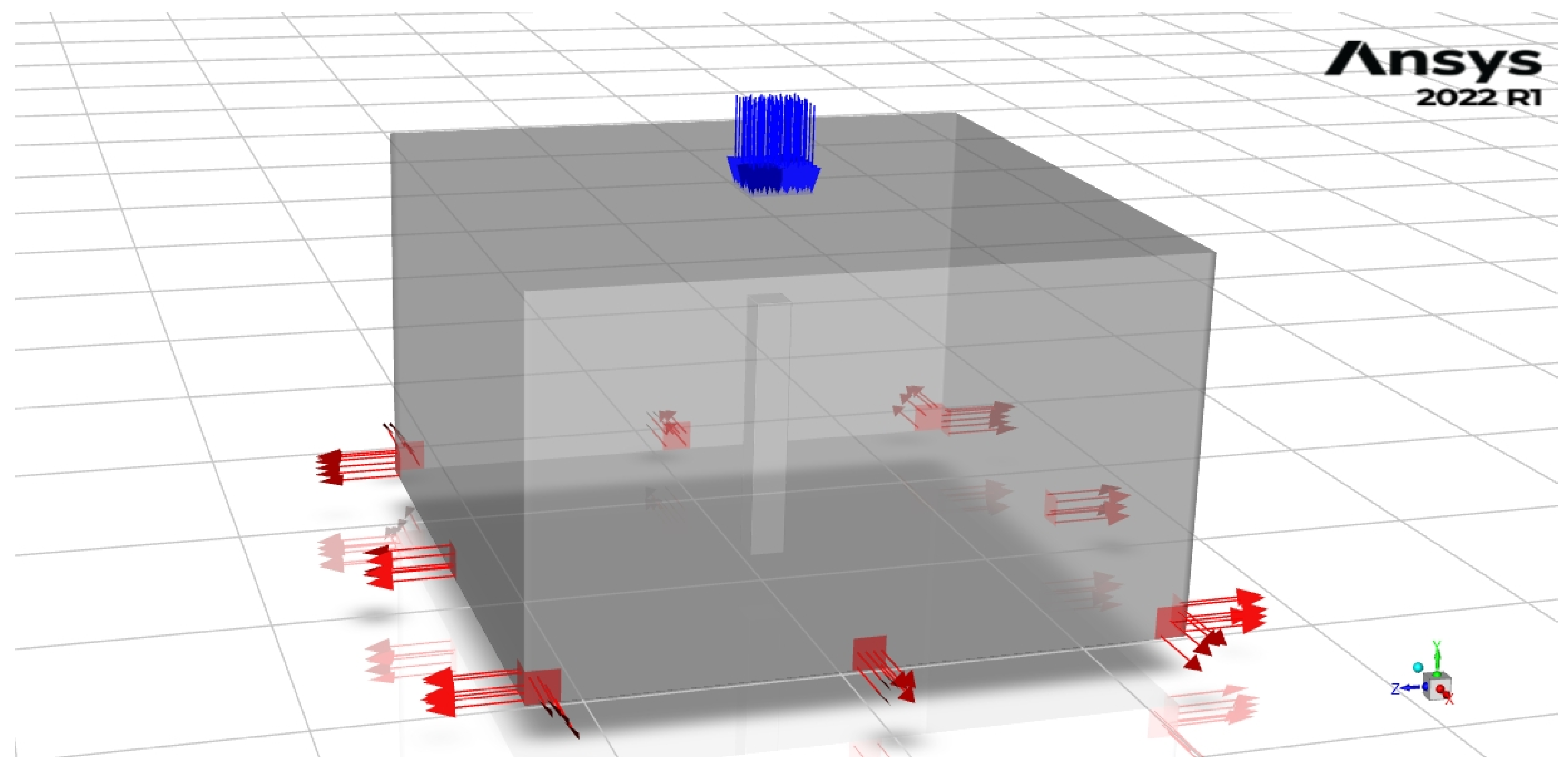
2.1. Geometry and General Setup of the Simulation

The room size was $4 \mathrm{m}\times 4 \mathrm{m}\times 2.35 \mathrm{m}$ (length × width × height) and represented a typical room of $16 {\mathrm{m}}^2$, for example, an office or a domestic room. This made the findings of this paper applicable to a wide range of scenarios. The room had a ventilation inlet in the ceiling and several outlets in the walls just above the floor. The inlet was divided into four separate streams, each pointing into one bottom corner of the room. This way, the occupant was not exposed to the direct air stream. This ventilation configuration was based on Xu and Raman [13]. Figure 1 shows an illustration of the room with the inlet and the outlets. For more detailed information, see Appendix A.1. The volume flow was $500 {\mathrm{m}}^3/\mathrm{h}$. There were two $0.6 \mathrm{m}\times 0.6 \mathrm{m}$ IR heaters placed in the middle of the wall, opposing each other; their maximum power output was at $324 \mathrm{W}$, resulting in a maximum area specific power output of 900 W m⁻². There was one occupant standing in the middle of the room, simplified as a rectangular cuboid, with a metabolic rate of $80 \mathrm{W}/{\mathrm{m}}^2$ ($1.38 \mathrm{met}$) and a total surface area of $1.5 {\mathrm{m}}^2$.

2.2. Design of Experiments

Design of Experiments summarizes a toolbox that is used in experiments and simulations to gain as much knowledge from as few data as possible. Commonly used Design of Experiment plans supply either linear or quadratic description models, meaning that they assume a linear or a quadratic correlation between an experimental input factor and the measured output quantity. To be able to choose the right simulation plan, a first set of test simulations was run and showed that the PMV description function was not linear; thus, we chose a design that allowed for a quadratic function to be fitted. This behavior was expected, because the emitted radiation energy of a surface increases with $T^4$, where T is the temperature of the surface. There are two commonly used designs for quadratic correlations, the Central Composite Design and the Box–Behnken Design.

To create the simulation plan, we used a CCD since compared to a Box Behnken Design, it allowed us to evaluate the corner points of the factor space, which provided better information in the relevant area [19]. The range of the four factors was selected to approximate values for winter conditions. All four factors’ boundary conditions were set in the simulation and therefore did not automatically change if another factor was changed. The wall was defined as a surface and had no volume and no thermal mass. The factors were as follows:

• Wall temperature, including ceiling and floor: $T_{\mathrm{Wall}}=13–20 °\mathrm{C}$
• Air inlet temperature: $T_{\mathrm{Inlet}}=15–23 °\mathrm{C}$
• Wall emissivity, including ceiling and floor: $ϵ=0.1–0.9$
• Area specific heating power: $P_{\mathrm{IR}}=100–900 \mathrm{W}/{\mathrm{m}}^2$ ($P_{\mathrm{IRtotal}}=72–648 \mathrm{W}$)

To use the results of the CCD to create a response surface, it is necessary to codify the parameters first. The use of codified parameters improves the numerical stability of the model fit and helps to understand and compare the effects of different factors on the response variable without being influenced by the original measurement units. To codify the parameters, the mean value was set to zero, and the upper and lower limits were set to the codified distance $+\alpha$ and $-\alpha$. The value for $\alpha$ was calculated by using:

$$\begin{array}{c}\hfill \alpha =\sqrt{\frac{\sqrt{Nf}-f}{2}}\end{array}$$

(1)

where $N=f+\left(2k\right)+n_0$ and $f=2^k$. $n_0$ is the number of center points; k the number of factors. For four parameters and three center points, $\alpha =1.547$. The codified simulation plan is displayed in Appendix A.2, the uncodified simulation plan in

Table 1. Simulation plan with four parameters and three center points (CPs). Simulation results for $T_{\mathrm{Air}}$, $T_{\mathrm{Dummy}}$, and PMV.

No.	${\mathit{T}}_{\mathbf{Wall}}$	${\mathit{T}}_{\mathbf{Inlet}}$	$\mathit{ϵ}$	${\mathit{P}}_{\mathbf{IR}}$	${\mathit{T}}_{\mathbf{Air}}$	${\mathit{T}}_{\mathbf{Dummy}}$	PMV
	$°\mathrm{C}$	$°\mathrm{C}$	-	$\mathrm{W}/{\mathrm{m}}^2$	$°\mathrm{C}$	$°\mathrm{C}$	-
1	14.24	16.41	0.24	241.4	16.24	24.20	−0.46
2	14.24	21.59	0.24	241.4	19.45	26.33	0.21
3	18.76	16.41	0.24	241.4	17.94	25.80	0.03
4	18.76	21.59	0.24	241.4	21.13	28.89	0.98
5	14.24	16.41	0.76	241.4	16.23	23.45	−0.68
6	14.24	21.59	0.76	241.4	19.43	25.55	−0.02
7	18.76	16.41	0.76	241.4	17.92	25.30	−0.12
8	18.76	21.59	0.76	241.4	21.10	28.20	0.78
9	14.24	16.41	0.24	758.6	16.62	25.82	0.01
10	14.24	21.59	0.24	758.6	19.80	27.86	0.66
11	18.76	16.41	0.24	758.6	18.34	27.05	0.40
12	18.76	21.59	0.24	758.6	21.51	30.57	1.47
13	14.24	16.41	0.76	758.6	16.51	24.30	−0.43
14	14.24	21.59	0.76	758.6	19.74	26.19	0.17
15	18.76	16.41	0.76	758.6	18.30	25.77	0.02
16	18.76	21.59	0.76	758.6	21.45	28.93	1.00
17	16.5	19	0.5	100	18.52	26.16	0.14
18	16.5	19	0.5	900	19.08	27.39	0.51
19	16.5	19	0.1	500	18.97	29.65	1.16
20	16.5	19	0.9	500	18.87	26.17	0.15
21	13	19	0.5	500	17.55	24.62	−0.32
22	20	19	0.5	500	20.08	27.88	0.67
23	16.5	15	0.5	500	16.31	24.18	−0.47
24	16.5	23	0.5	500	21.34	28.06	0.74
25 (CP1)	16.5	19	0.5	500	18.83	26.8	0.33
26 (CP2)	16.5	19	0.5	500	18.83	26.8	0.33
27 (CP3)	16.5	19	0.5	500	18.83	26.8	0.33

. It included 16 corner points, representing a cube in the factor space, 8 star points, and 3 center points.

The basic quadratic response surface function for a CCD with 4 factors is given in Appendix A.3. The parameters were fitted using a multiple linear regression analysis with the result data from the simulation.

2.3. Model

Simulations were run in Ansys Fluent within the Ansys Workbench (2022 R1). Due to the two symmetry planes, only one quarter of the room was simulated. Although the conditions in the room dynamically change when the IR heater was turned on or off, we performed steady-state simulations. This approach was justified because the temperature changes in the room could be considered quasi-stationary for two reasons: first, the room responded slowly to changes in heating power, and second, the IR heater could quickly adjust its power output according to the room’s conditions. In a real-life scenario, a controller would adapt the IR heater power to the new optimal set point before the conditions in the room would change noticeably. To allow for different air temperatures in the steady-state simulations, we introduced the inlet temperature $T_{\mathrm{Inlet}}$ to our simulations. This way, it was possible to run steady-state simulations at different air temperatures for the same set of parameters (only changing $T_{\mathrm{Inlet}}$). Meshing was performed using the Assembly Meshing—Cut Cell function in Ansys Mesh, resulting in a hexahedral dominant mesh with 158,179 elements. To validate the mesh, we performed a mesh refinement study which showed no mesh dependency on the results. For more details on the simulation, see Appendix A.1

3. Results and Discussion

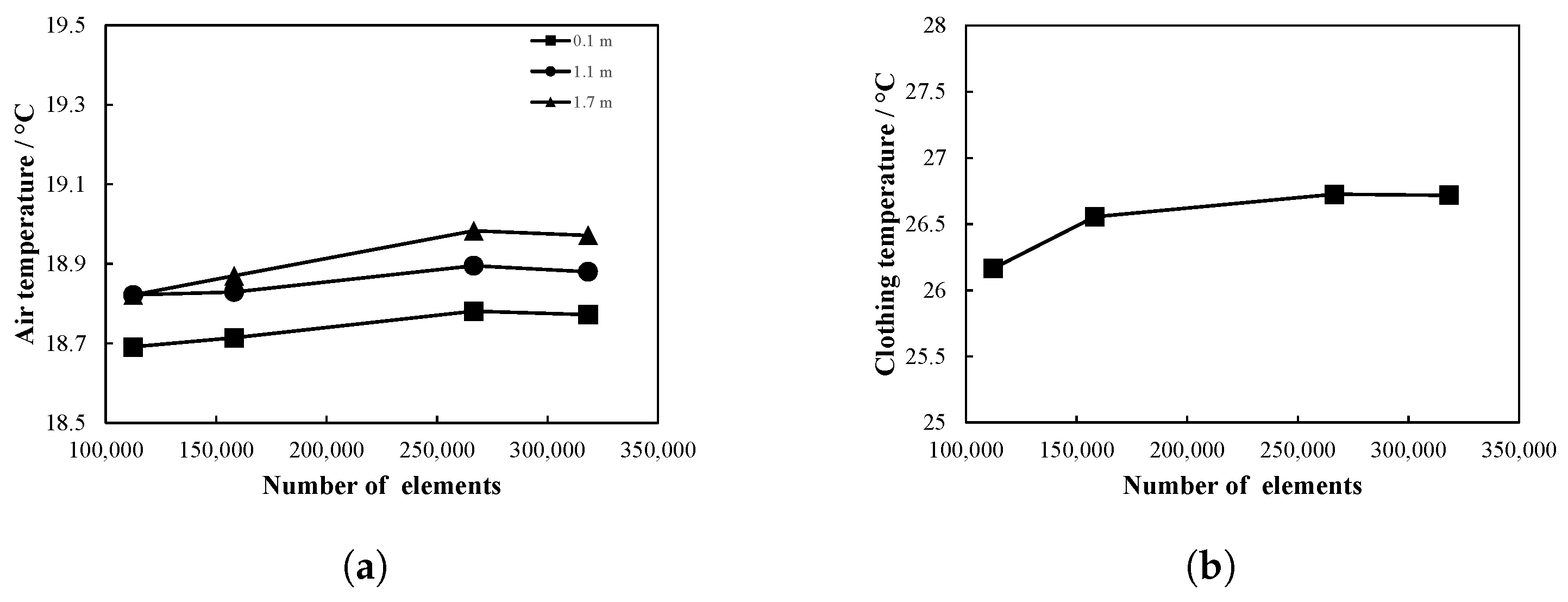
In the first part of the results section, we present the outcome of the simulation; in the second, we construct the response surface function to calculate the PMV for any given condition.

3.1. Simulation

The uncodified parameters as well as the results of the simulation are shown in Table 1, where the first 16 data points represent the corners of the cube while points 17–24 are the star points of the CCD, 2 for each parameter. The PMV was calculated with “pythermalcomfort” [20] using the average surface temperature of the occupant $T_{\mathrm{Dummy}}$ in the room and equating it with the clothing surface temperature in the PMV formula. The air temperature $T_{\mathrm{Air}}$ was the average air temperature in the room, the metabolic rate was at $1.38 \mathrm{met}$, the clothing value at $1 \mathrm{clo}$, the relative humidity was assumed to be $50\%$, the air velocity around the dummy was approximated as $0.1 \mathrm{m}/\mathrm{s}$.

In Table 1, we can see that the PMV increased if the wall emissivity $ϵ$ was decreased (while the other parameters were kept constant). Points to mention here are the eight pairs from the cube points where only the emissivity changed, 1 and 5, 2 and 6, etc., as well as the star points 19 and 20. The increase in PMV was because the surrounding walls absorbed less IR radiation and instead reflected it back to the occupant inside the room. This fact suggested that the underlying assumption of yielding a higher PMV by only decreasing the emissivity was correct. Another point to mention is that the impact of the emissivity on the PMV was greater for the higher IR heating power. For example, changing the emissivity only between data points 1 and 5, the difference in PMV was $(-0.46)-(-0.68)=0.22$, while at points 9 and 13 (same parameters, but higher heating power), the difference was $0.01-(-0.43)=0.44$. This suggested that with an increased IR heating power, the impact of reflective wall coatings became more significant, as there was more radiant heat to be reflected, leading to an overall increased radiant temperature. The opposite applied to the wall temperature: the impact of the emissivity on the PMV was bigger for lower wall temperatures than it was for high wall temperatures as can be seen by comparing the difference between points 1 and 5 and point 3 and 7: $(-0.46)-(-0.68)>0.03-(-0.12)$. This was due to the higher radiant heat exchange with the occupant at lower wall temperatures.

The graph in Figure 2 shows the two star points and the center point at $ϵ=[0.1;0.5;0.9]$ (points 19, 20, and 25). All other parameters are constant at a medium value. The data cover the entire range for $ϵ$ and show a non-linear correlation, which supports the decision of choosing a quadratic response surface model. The value $ϵ=0.9$ matches the most common building materials, whereas $ϵ=0.1$ represents a highly reflective wall coating. At $ϵ=0.9$, $\mathrm{PMV}=0.15$, which is within the boundaries of acceptable thermal comfort. However, at $ϵ=0.1$, $\mathrm{PMV}=1.16$, an increase beyond the acceptable threshold resulting in a PPD of $35\%$. The change in emissivity accounts for a difference in PMV of $1.16-0.15=1.01$, which is equal to an air temperature rise of $9.7 \mathrm{K}$ (using the PMV formula, raising only the air temperature until PMV increases from $0.15$ to $1.16$, while keeping all other parameters constant). Even before using a response surface method, it becomes clear that the results show energy saving potential for the combination of IR reflective walls and IR heaters.

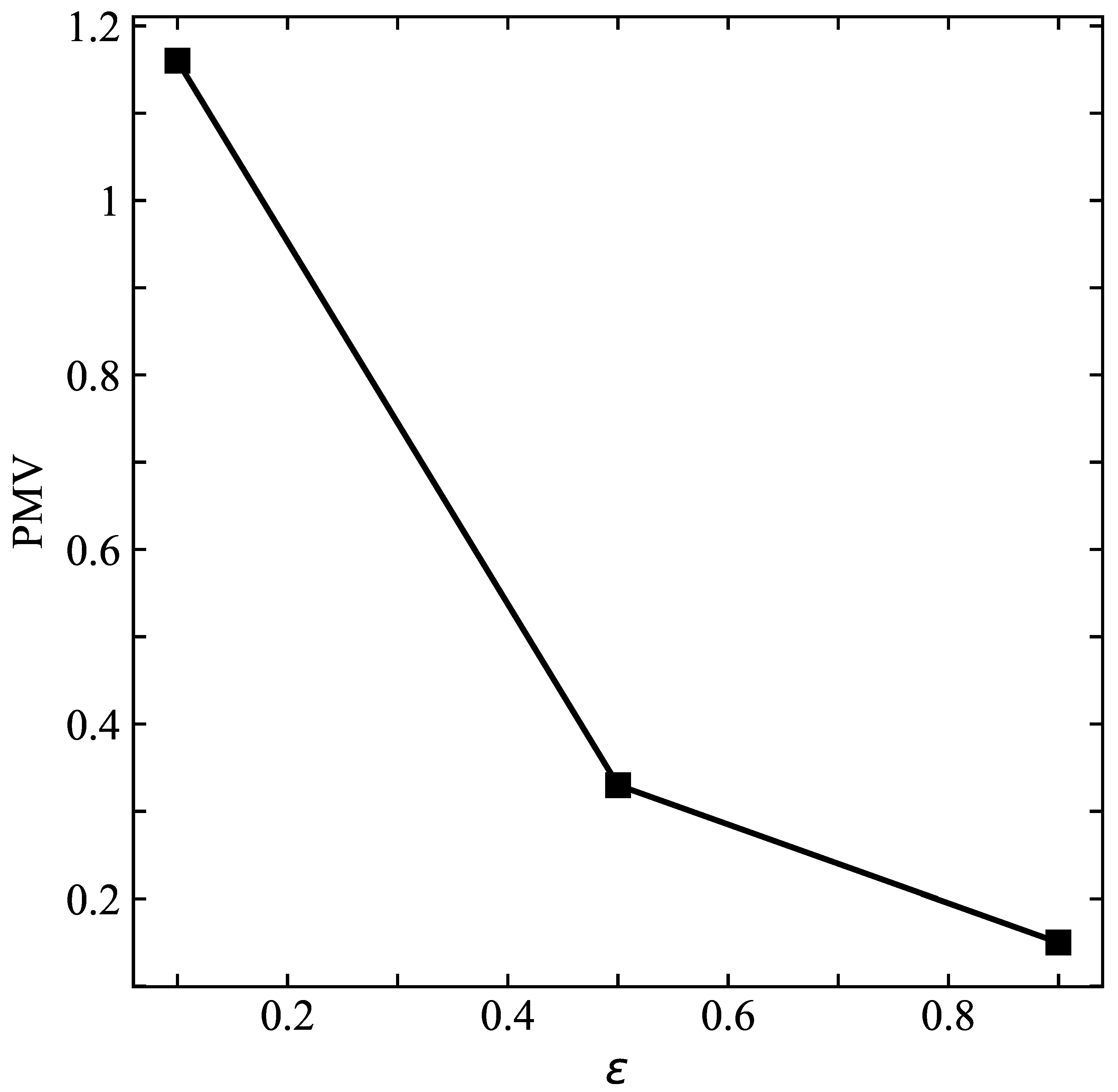
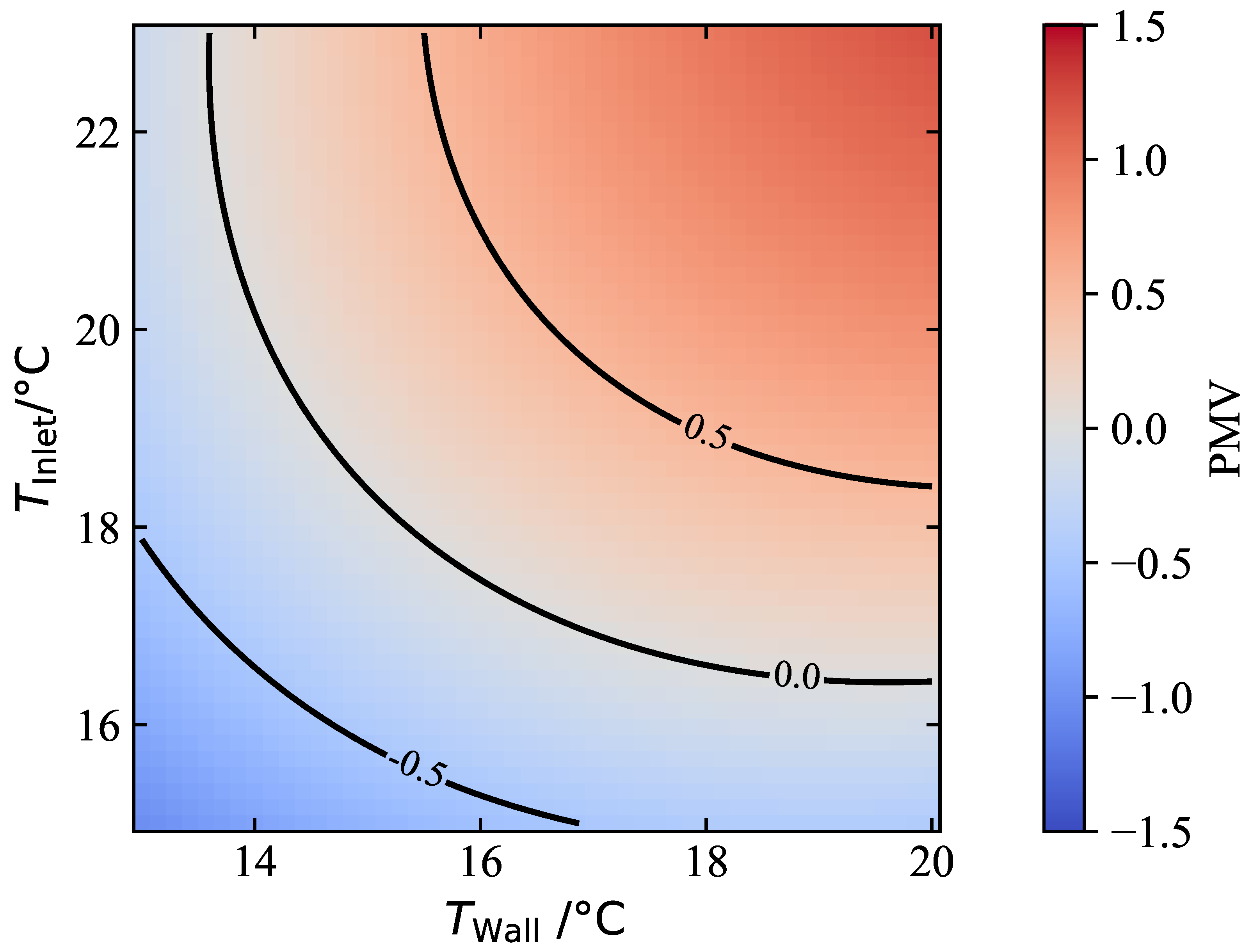
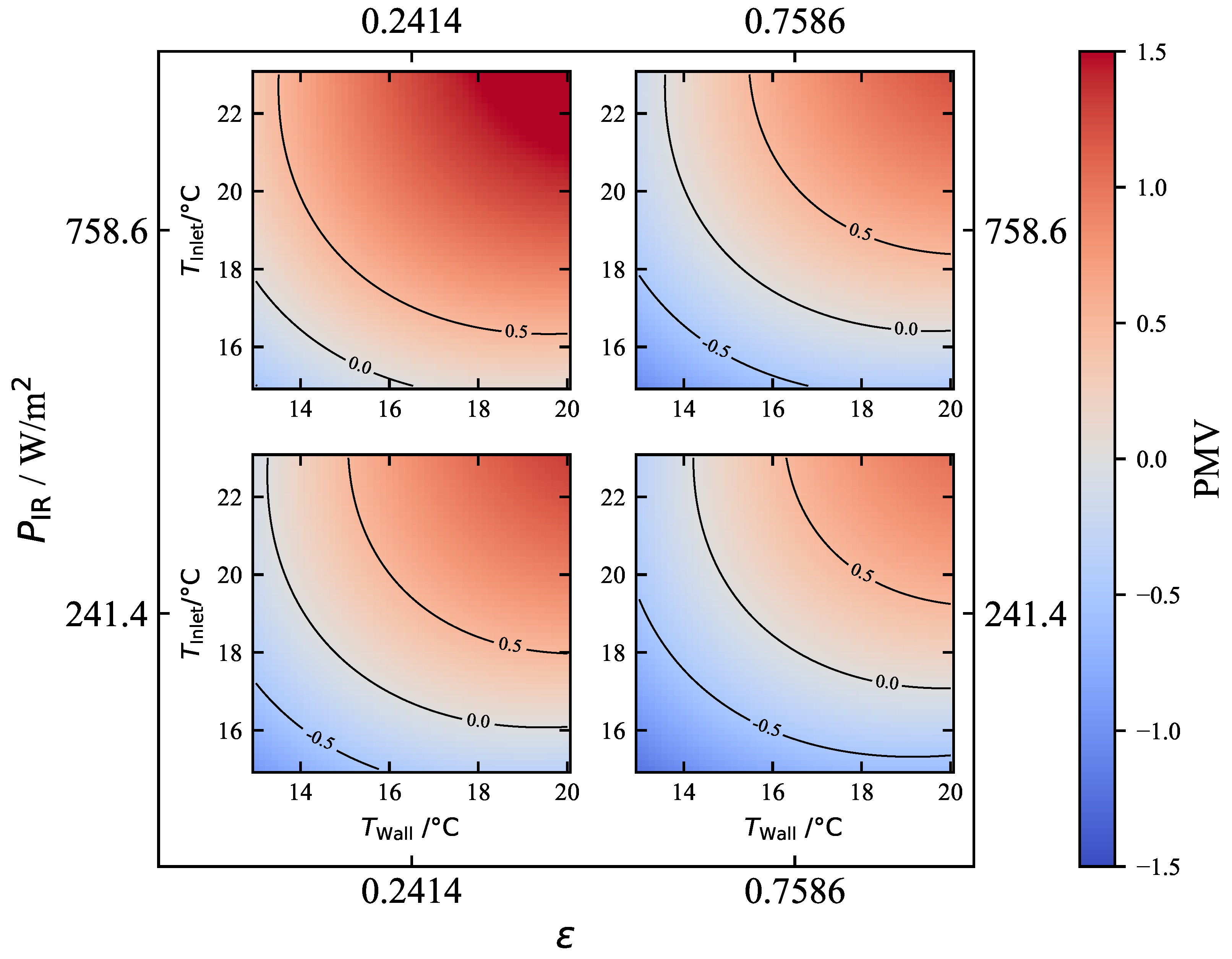
3.2. Response Surface

In this step, we fit the response surface $\mathrm{PMV}=f(T_{\mathrm{Wall}},T_{\mathrm{Inlet}},ϵ,P_{\mathrm{IR}})$ to be able to calculate the $\mathrm{PMV}$ for any given input parameter combination. For the underlying equation, see Appendix A.3. To fit the response surface, we used multiple linear regression. The p-value was kept below $0.05$; all other terms were left out from the final equation one by one. Note that the inputs to Equation (2) are in the codified form.

$$\begin{array}{cc}\hfill \mathrm{PMV}=& 0.3384\hfill \\ \hfill & +0.319 T_{\mathrm{Wall}}-0.0861 T_{\mathrm{Wall}}^2\hfill \\ \hfill & +0.4018 T_{\mathrm{Inlet}}-0.1028 T_{\mathrm{Inlet}}^2\hfill \\ \hfill & -0.1993 ϵ+0.1146 {ϵ}^2+0.1517 P_{\mathrm{IR}}\hfill \\ \hfill & +0.0825 T_{\mathrm{Wall}}{T}_{\mathrm{Inlet}}-0.0613 ϵP_{\mathrm{IR}}\hfill \end{array}$$

(2)

The function can be displayed in a heat-map surface plot, where two parameters are kept at a constant level. Figure 3 shows such a response surface for constant $ϵ=0.5$ and $P_{\mathrm{IR}}=500 \mathrm{W}/{\mathrm{m}}^2$. The contour lines indicate the range for acceptable thermal comfort with PMV values between $-0.5$ and $0.5$. As already seen in the raw simulation results, the PMV increases for higher wall and inlet temperatures. This representation of the data can be used to operate IR heaters to keep the PMV within the boundaries of the contour lines.

To further understand the behavior of the response surface function, the heat maps in Figure 4 show how the temperature range for optimal thermal comfort shifts when changing the emissivity and the heating power. Reading the inlet temperature $T_{\mathrm{Inlet}}$ from the heat maps at $\mathrm{PMV}=0$ and $T_{\mathrm{Wall}}=16.5 °\mathrm{C}$ gives:

• $T_{\mathrm{Inlet},ϵ=0.7586,P_{\mathrm{IR}}=241.4 \mathrm{W}/{\mathrm{m}}^2}=18 °\mathrm{C}$
• $T_{\mathrm{Inlet},ϵ=0.2414,P_{\mathrm{IR}}=241.4 \mathrm{W}/{\mathrm{m}}^2}=16.7 °\mathrm{C}$
• $T_{\mathrm{Inlet},ϵ=0.7586,P_{\mathrm{IR}}=758.6 \mathrm{W}/{\mathrm{m}}^2}=17.1 °\mathrm{C}$
• $T_{\mathrm{Inlet},ϵ=0.2414,P_{\mathrm{IR}}=758.6 \mathrm{W}/{\mathrm{m}}^2}=15 °\mathrm{C}$

By reducing the emissivity from $0.7586$ to $0.2414$ at $P_{\mathrm{IR}}=241.4 \mathrm{W}/{\mathrm{m}}^2$, the inlet temperature can be lowered by $1.3 °\mathrm{C}$ which is a greater effect than tripling the heating power from $241.4 \mathrm{W}/{\mathrm{m}}^2$ to $758.6 \mathrm{W}/{\mathrm{m}}^2$, where an inlet temperature drop of only $0.9 °\mathrm{C}$ is possible to maintain an optimal PMV. Raising the heating power and reducing the inlet temperature at the same time allows for the biggest change in inlet temperature of $3 °\mathrm{C}$, further underlining the energy saving potential of low-emissivity surfaces and IR heaters.

While Equation (2) provides a PMV value depending on all four input parameters including the inlet temperature $T_{\mathrm{Inlet}}$, $T_{\mathrm{Inlet}}$ is a parameter introduced in the simulations only to be able to run steady-state simulations at different air temperatures. In most applications, the air temperature is the relevant variable for determining thermal comfort and therefore has to replace the inlet temperature. To solve this problem, we created another surface response function from the simulations, in which $T_{\mathrm{Air}}=f(T_{\mathrm{Wall}},T_{\mathrm{Inlet}},ϵ,P_{\mathrm{IR}})$. Thus, it was possible to obtain the corresponding air temperature for a calculated PMV. The surface response function, see Equation (3), was created following the same steps as for the PMV.

$$\begin{array}{cc}\hfill T_{\mathrm{Air}}=& 18.82 °\mathrm{C}\hfill \\ \hfill & +0.8459 T_{\mathrm{Wall}}+1.6019 T_{\mathrm{Inlet}}\hfill \\ \hfill & -0.0241 ϵ+0.0396 {ϵ}^2+0.1773 P_{\mathrm{IR}}\hfill \end{array}$$

(3)

Now, with the function for $T_{\mathrm{Air}}$ and PMV, it is possible to determine the optimal heating power for any given parameters. Implemented in a power control, this could serve as a power control mechanism, similar to a heating curve. Instead of adjusting the supply temperature of the heating system to the outside temperature, with this function, it is possible to adjust the heating power to the present room conditions and status of occupancy.

Nonetheless, the simulation overlooked elements such as furniture, windows, and other obstructions within the room, factors that could impede the effectiveness of reflective wall paints. In a practical setting, it would be necessary to establish a cumulative average value for the emissivity in a room, considering all surfaces and their respective emissivities. Additionally, the absorption of IR radiation in the air could diminish the potential for energy savings. Another crucial consideration involves humidity. Lowering the air temperature and preventing the outer wall from absorbing IR radiation may result in moisture accumulation and mold formation. This, in turn, could make additional ventilation necessary, which would cause higher ventilation losses.

4. Conclusions

This research demonstrated that the integration of IR heaters with reflective walls had the potential to minimize energy consumption by curbing heat losses and maintaining acceptable thermal comfort at lower air temperatures. The combined impact of increased radiant temperatures and decreased air temperatures, particularly in spaces with intermittent occupancy, offers a promising solution. This is especially noteworthy given the swift response times of IR heaters, offering the potential for optimized operation.

The study utilized a CCD for an efficient exploration of the factor space, allowing for the creation of a response surface function. Simulation results and the derivation of a response surface function provided valuable insights into the interplay of the factors: wall temperature, inlet temperature, wall emissivity, and heating power. Creating a second response surface for the air temperature opens the possibility for practical applications. This innovative approach, building upon previous studies, opens ways for the development of control systems that can dynamically adapt IR heater settings based on real-time conditions. The potential to implement this technology in real building applications offers a sustainable alternative to conventional heating systems, aligning with the global pursuit of energy-efficient and environmentally conscious building practices.

To conclude, the integration of IR heaters with IR reflective walls presents a promising alternative or supplement to conventional heating systems, contributing to both energy efficiency and occupants’ comfort. Future work could focus on conducting experimental validations to further advance the applicability of this approach in diverse real-world scenarios and to implement it in energy building simulations, estimating the yearly energy saving potential for different climates and buildings.

References

1. King, D. Engineering a Low Carbon Built Environment: The Discipline of Building Engineering Physics; The Royal Academy of Engineering: London, UK, 2010. [Google Scholar]
2. Shafiee, S.; Topal, E. A long-term view of worldwide fossil fuel prices. Appl. Energy 2010, 87, 988–1000. [Google Scholar] [CrossRef]
3. Statista Research Department. Durchschnittlicher Verbraucherpreis für Leichtes Heizöl in Deutschland in den Jahren 1960 bis 2024. Available online: https://de.statista.com/statistik/daten/studie/2633/umfrage/entwicklung-des-verbraucherpreises-fuer-leichtes-heizoel-seit-1960/ (accessed on 8 April 2024).
4. Bergman, N. Why is renewable heat in the UK underperforming? A socio-technical perspective. Proc. Inst. Mech. Eng. Part A J. Power Energy 2013, 227, 124–131. [Google Scholar] [CrossRef]
5. Opel, O. Warmwasserbereitung als Hemmschuh der Energiewende—Technische, Hygienische und Rechtliche Konfliktpunkte Zwischen Wärmepumpeneinsatz und Trinkwarmwasserbereitung; Gesellschaft für Energie und Klimaschutz Schleswig-Holstein GmbH: Kiel, Germany, 2023. [Google Scholar]
6. Heider, J.; Conrad, N.; Stark, T.; Abdulganiev, A.; Kosack, P.; Wagner, A.K. Forschungsprojekt IR Bau; HTWG Konstanz: Konstanz, Germany, 2020. [Google Scholar]
7. Fanger, P.O. Thermal Comfort: Analysis and Applications in Environmental Engineering; McGraw-Hill: New York, NY, USA, 1970. [Google Scholar]
8. ISO 7730:2005; Ergonomics of the Thermal Environment—Analytical Determination and Interpretation of Thermal Comfort Using Calculation of the PMV and PPD Indices and Local Thermal Comfort Criteria. Technical Report. International Organization for Standardization: Geneva, Switzerland, 2005.
9. Kosack, P. Leitfaden Infrarotheizung; IG Infrarot Deutschland: Sauerlach, Germany, 2021. [Google Scholar]
10. Statistisches Bundesamt. 57% der im Jahr 2022 Gebauten Wohngebäude Heizen mit Wärmepumpen. Available online: https://www.destatis.de/DE/Presse/Pressemitteilungen/2023/06/PD23_N034_31121.html (accessed on 19 October 2023).
11. Lazzarin, R. Dual source heat pump systems: Operation and performance. Energy Build. 2012, 52, 77–85. [Google Scholar] [CrossRef]
12. Bundesamt für Wirtschaft und Ausfuhrkontrolle. Bundesförderung für Effiziente Gebäude—Infoblatt zu den Förderfähigen Maßnahmen und Leistungen. Available online: https://www.bafa.de/SharedDocs/Downloads/DE/Energie/beg_infoblatt_foerderfaehige_kosten.html (accessed on 1 December 2023).
13. Xu, J.; Raman, A.P. Controlling radiative heat flows in interior spaces to improve heating and cooling efficiency. iScience 2021, 24, 102825. [Google Scholar] [CrossRef] [PubMed]
14. Malz, S.; Krenkel, W.; Steffens, O. Infrared reflective wall paint in buildings: Energy saving potentials and thermal comfort. Energy Build. 2020, 224, 110212. [Google Scholar] [CrossRef]
15. Gläser, H. Improved insulating glass with low emissivity coatings based on gold, silver, or copper films embedded in interference layers. Glass Technol. 1980, 21, 254–261. [Google Scholar]
16. Verbraucherzentrale Thüringen. Energiesparfarbe: Zu Schön, um Wahr zu Sein. Available online: https://www.vzth.de/pressemeldungen/energie/energiesparfarbe-zu-schoen-um-wahr-zu-sein-82255 (accessed on 4 October 2023).
17. Verbraucherzentrale Thüringen. Verbraucherzentrale Energieberatung Warnt vor „Energiesparfarbe“. Available online: https://wdvs.enbausa.de/nachrichten/verbraucherzentrale-energieberatung-warnt-vor-energiesparfarbe (accessed on 4 October 2023).
18. Kosack, P. Beispielhafte Vergleichsmessung Zwischen Infrarotstrahlungsheizung und Gasheizung im Altbaubereich; TU Kaiserslautern: Kaiserslautern, Germany, 2009. [Google Scholar]
19. Siebertz, K.; van Bebber, D.; Hochkirchen, T. Statistische Versuchsplanung: Design of Experiments (DoE); VDI-Buch; Springer: Berlin/Heidelberg, Germany, 2017. [Google Scholar]
20. Tartarini, F.; Schiavon, S. pythermalcomfort: A Python package for thermal comfort research. SoftwareX 2020, 12, 100578. [Google Scholar] [CrossRef]
Figure 1. Schematic illustration of the room with the air in- and outlets; in the middle, the cuboid represents an occupant.
Buildings 14 02183 g001
Figure 2. Simulation results at constant values P IR = 500   W / m 2 , T Wall = 16.5   ° C , and T Inlet = 19   ° C at the two star points and the center point.
Buildings 14 02183 g002
Figure 3. Response surface for P IR = 500   W / m 2 and ϵ = 0.5 .
Buildings 14 02183 g003
Figure 4. Response surfaces for combinations with heating power P IR = 241.4   W / m 2 and P IR = 758.6   W / m 2 and surface emissivity ϵ = 0.2414 and ϵ = 0.7586 .
Buildings 14 02183 g004