Influence of Ground Motion Non-Gaussianity on Seismic Performance of Buildings

Abstract

The non-Gaussian feature of seismic ground motion has been reported in some works. However, there remains a lack of research on the influence of the ground motion non-Gaussianity on the seismic performance of buildings, which motivates this study. By employing a non-Gaussian non-stationary random process simulation method previously proposed by the authors, 40,000 ground motion acceleration signals are efficiently generated, including 20,000 Gaussian and 20,000 non-Gaussian records. As computational examples, a four-story frame building and a three-tower super-tall building are selected. The generated acceleration signals serve as external excitations for the two buildings, allowing for a comparison of the differences in seismic structural responses caused by the Gaussian and non-Gaussian earthquake groups. Probability analysis is performed using top-layer displacement and maximum inter-story drift ratio as damage indicators. The results show that the structural responses induced by both Gaussian and non-Gaussian earthquake groups have identical first- and second-order moments but different higher-order moments. The responses from non-Gaussian earthquakes display distinct non-Gaussian traits, with their distribution of extreme values exhibiting a longer tail compared to the Gaussian counterparts. This leads to a notably larger value of non-Gaussian responses under high crossing probabilities, with an amplification that can surpass 18%.

1. Introduction

Earthquake ground motion is a typical instance of the stochastic process. The recorded signal represents only a single sample realization from the underlying stochastic process [1,2]. Consequently, future ground motion remains uncertain, highlighting the importance of performing stochastic analysis during the structural seismic design phase. Conventionally, ground motion is often assumed to follow a non-stationary Gaussian process, disregarding the time-varying characteristics in higher-order moments. However, some research has revealed evident non-Gaussian attributes in recorded seismic ground motion [3,4], and a non-Gaussian model can accurately capture the inherent variability of ground motion parameters [5]. Therefore, both non-stationarity and non-Gaussianity should be duly considered in structural seismic analysis.

Previous analyses of structural seismic performance heavily rely on the utilization of measured seismic ground motion signals [6,7,8,9,10,11,12]. This methodology involves employing seismic ground motion records obtained from actual earthquakes as external excitations to evaluate the seismic response of the target structure and facilitate the optimal design of seismic systems [13,14]. Nonetheless, this approach encounters a notable challenge: the limited availability of real earthquake signals restricts the sample size, making it inadequate for achieving probabilistic analysis of the random vibration response induced by earthquakes. To overcome the challenge of limited seismic motion samples, various methodologies have been proposed. These methods can be broadly classified into several categories: (1) Ground motion modification methods [14,15,16,17] involve adjusting and rescaling real seismic motion records based on temporal or frequency characteristics to obtain simulated signals. (2) The Bayesian updating model methods [18,19] approximate the posterior distribution of engineering demand parameters based on a small number of available seismic motion records. (3) The stochastic dynamics methods [20,21,22] rely on some ideal assumptions to mathematically derive the probability functions for structural response. Despite the availability of the above methods for solving some problems, the Monte Carlo simulation method remains the benchmark for assessing their accuracy and reliability. In addition, the Monte Carlo simulation stands out as the only universally applicable approach capable of providing accurate solutions, even in cases involving non-linearity, non-stationarity, and non-Gaussianity.

The Monte Carlo method is built upon the fundamental principle of simulating sample realizations from underlying stochastic processes. In recent years, many simulation algorithms have been proposed to generate seismic ground motion signals [23,24,25,26,27]. These approaches enable the artificial adjustment of simulation parameters based on target operating conditions and the rapid generation of a large number of ground motions with the same simulation objectives. With the support of increasingly advanced computational techniques and hardware, structural responses can be obtained by numerical calculation, such as the commonly used finite element method, thereby facilitating probabilistic analysis of seismic performance. However, the seismic ground motion simulation algorithms utilized in the aforementioned studies have primarily focused on the non-stationary properties of ground motion. They typically assume the underlying process to be a non-stationary Gaussian random process, prioritizing the time-varying characteristics of the first two order statistical moments, namely mean, variance, and power spectral density (PSD). Nevertheless, these approaches tend to overlook the potential temporal variations of higher-order statistical moments, particularly skewness and kurtosis [28]. The reasons behind this issue can be attributed to two main factors. Firstly, there has been insufficient attention given to the non-Gaussian characteristics of seismic ground motions. Secondly, the simulation of non-Gaussian non-stationary random processes poses considerable technical challenges, resulting in a scarcity of available simulation algorithms.

Recently, several algorithms have been developed for simulating non-Gaussian non-stationary random processes, such as those based on Karhunen–Loeve expansions [29,30,31] or spectral representation methods [1,32]. However, most of them involve computationally intensive iterative calculations. To address this limitation, the authors of this study proposed a novel simulation algorithm [2] based on the Time-Varying Auto-Regressive (TVAR) model. Unlike existing approaches, this algorithm eliminates the need for iterative computations. As a result, it enables rapid and efficient simulation of single-point seismic ground motions, making it highly promising for the seismic performance analysis of building structures. It must be acknowledged that although ground motion simulation technology has made significant advancements, artificially simulated seismic signals are still unable to fully replicate the complexity and variability of real seismic events. Therefore, the seismic design of structures still needs to refer to actual earthquake signals.

Although some notable progress has been made in the simulation of non-Gaussian non-stationary seismic ground motion signals, there remains a lack of research on the influence of non-Gaussian characteristics on the seismic performance of buildings. Therefore, this study aims to fill this gap and provide some valuable insights. Different from previous research, this study applies artificial ground motions that not only possess time-varying second-order statistics but also have time-varying third- and fourth-order statistics. This implies that these simulations exhibit both non-stationary and non-Gaussian properties. Thus, the resultant structural responses are also characterized by non-stationarity and non-Gaussianity, enabling a detailed examination of the higher-order statistical attributes of structural responses.

The main framework of this paper is outlined as follows: Firstly, utilizing the rapid simulation algorithm proposed by the authors, a large quantity of non-Gaussian seismic time histories is generated with specific targets of evolutionary power spectral density (EPSD) and time-varying skewness and kurtosis. Secondly, an equal number of Gaussian seismic ground motions are generated with the same EPSD as a comparative benchmark. Thirdly, two structures, a four-story frame structure and a multi-tower high-rise building, are chosen as case studies. The generated Gaussian and non-Gaussian ground motions are implemented as external excitations on these structures, and the responses are obtained. Finally, some important damage indicators, such as maximum displacement and inter-story drift ratio, are compared between the two sets of seismic ground motions to assess the influence of non-Gaussian characteristics on the seismic performance of buildings.

2. Simulation of Non-Gaussian Non-Stationary Ground Motions

2.1. Brief Review of the Simulation Algorithm

The authors have previously proposed an efficient simulation algorithm for non-Gaussian non-stationary stochastic processes which are defined by EPSD and time-varying skewness and kurtosis, as presented in reference [2]. In this study, we will employ this algorithm to generate a database of non-Gaussian ground motion signals. The purpose is to investigate the impact of non-Gaussian characteristics on the seismic performance of buildings. The central idea of the algorithm revolves around utilizing the TVAR model to transform non-Gaussian white noise, characterized by time-varying first four-order statistical moments, into the desired stochastic process. Some important procedures are briefly reviewed in this section.

Step 1: Calculate the target non-stationary auto-correlation function (NACF). According to the evolutionary spectrum theory [33], the NACF of a non-stationary process $x\left(t\right)$ can be represented by the following expression:

$$R_{xx}\left(\mathrm{v},t\right)=E\left[x\left(v\right)x\left(t\right)\right]={\displaystyle {\int }_{-\infty }^{\infty }\sqrt{s\left(\omega ,v\right)s\left(\omega ,t\right)}}{e}^{i\omega \left(v-t\right)}d\omega$$

(1)

where $s\left(\omega ,t\right)$ is the specified EPSD of $x\left(t\right)$, and $\omega$ is the circular frequency. Based on Equation (1), the desired NACF can be calculated.

Step 2: Establish a TVAR model. The TVAR model is expressed as [34]

$${\displaystyle \sum _{i=0}^p{a}_i\left(n\right)x\left(n-i\right)=w\left(n\right)}$$

(2)

where $p$ is the model order; $a_i\left(n\right)$ are time-varying coefficients, and $a_0\left(n\right)=1$; $x\left(n\right)$, the output of the model, is a discrete sample realization of $x\left(t\right)$ with a mean value of zero; $w\left(n\right)$, the input of the model, is a zero-mean white noise, with an NACF $R_{ww}\left(m,n\right)=0$ for $m\ne n$. The construction of a TVAR model involves two key steps: the selection of p and the determination of $a_i\left(n\right)$. The value of p is chosen based on the decay rate observed in the NACF. A smaller p indicates a faster rate of decay in the NACF. The specific strategy is suggested in reference [2]. By postmultiplying Equation (2) with $x\left(n-j\right)$ and taking expectations under the condition that $j=1, 2, \dots p$, we obtain

$$\left[\begin{array}{cccc}{R}_{xx}\left(n-1,n-1\right)& R_{xx}\left(n-2,n-1\right)& \cdots & R_{xx}\left(n-p,n-1\right)\\ R_{xx}\left(n-1,n-2\right)& R_{xx}\left(n-2,n-2\right)& \cdots & R_{xx}\left(n-p,n-2\right)\\ ⋮& ⋮& \ddots & ⋮\\ R_{xx}\left(n-1,n-p\right)& R_{xx}\left(n-2,n-p\right)& \cdots & R_{xx}\left(n-p,n-p\right)\end{array}\right]\left[\begin{array}{c}{a}_1\left(n\right)\\ a_2\left(n\right)\\ ⋮\\ a_p\left(n\right)\end{array}\right]=-\left[\begin{array}{c}{R}_{xx}\left(n,n-1\right)\\ R_{xx}\left(n,n-2\right)\\ ⋮\\ R_{xx}\left(n,n-p\right)\end{array}\right]$$

(3)

By solving Equation (3), the time-varying coefficients $a_i\left(n\right)$ can be computed for each time instant of $n=1, 2, 3\dots$.

Step 3: Determination of the time-varying first four-order moments of input. For a univariate, one-dimensional time series comprising $N$ time instants, the TVAR model describing the relationship between the output X and input W can be represented in a vector–matrix form as follows

$$A_{N\times N}{X}_{N\times 1}=W_{N\times 1}$$

(4a)

where

$$A_{N\times N}={\left[\begin{array}{ccccccc}{a}_0\left(1\right)& & & & & & \\ a_1\left(2\right)& a_0\left(2\right)& & & & & \\ ⋮& & \ddots & & & & \\ a_p\left(p+1\right)& \cdots & \cdots & a_0\left(p+1\right)& & & \\ 0& a_p\left(p+2\right)& \cdots & \cdots & a_0\left(p+2\right)& & \\ ⋮& & \ddots & & & \ddots & \\ 0& \cdots & \cdots & a_p\left(N\right)& \cdots & \cdots & a_0\left(N\right)\end{array}\right]}_{N\times N}$$

(4b)

and $X_{N\times 1}={\left[\begin{array}{cccc}x\left(1\right)& x\left(2\right)& \cdots & x\left(N\right)\end{array}\right]}^T$, $W_{N\times 1}={\left[\begin{array}{cccc}w\left(1\right)& w\left(2\right)& \cdots & w\left(N\right)\end{array}\right]}^T$. By inverting Equation (4a), it yields

$$X_{N\times 1}=H_{N\times N}{W}_{N\times 1}$$

(5)

where $H_{N\times N}=A_{N\times N}^{-1}$ is the impulse response matrix of the TVAR model. The connection between the first four-order moments of X and W can be succinctly expressed in a compact matrix formulation as [2]

$$E\left(X^l\right)=H^{l}E\left(W^l\right)+F$$

(6)

where $E\left(X^l\right)$ represents the marginal moment of X, with known values; $F=0$ for $l=1, 2 \mathrm{or} 3$; for $l=4$, $F=3E\left(X^2\right)\otimes E\left(X^2\right)-3H^4\left[E\left(W^2\right)\otimes E\left(W^2\right)\right]$, where the symbol $\otimes$ denotes element-by-element multiplication. From Equation (6), the marginal moments of W are obtained as

$$E\left(W^l\right)=H_{\ast }^l\left(E\left(X^l\right)-F\right)$$

(7)

where $H_{\ast }^l$ is the inverse of $H^l$. The time-varying skewness and kurtosis of the input can be calculated as follows:

$$S{K}_W={\displaystyle \frac{E\left(W^3\right)}{{\left[E\left(W^2\right)\right]}^{\raisebox{1ex}{$3$}\!\left/ \!\raisebox{-1ex}{$2$}\right.}}}$$

(8a)

$$K{U}_W={\displaystyle \frac{E\left(W^4\right)}{{\left[E\left(W^2\right)\right]}^2}}$$

(8b)

The time-varying first- to fourth-order moments of the input W can be determined so far.

Step 4: Generation of the non-Gaussian white noise input. The objective of this step is to generate non-Gaussian white noise input that possesses the desired time-varying first to fourth-order moments, as determined in Step 3. This can be effectively achieved by employing either the Johnson transformation model [35] or the Hermite polynomial model [36]. These models are commonly employed in engineering to address non-Gaussian challenges [37,38,39,40]. In this study, the Johnson transformation model is chosen as the preferred method due to its wider applicable range. In the interest of brevity, the detailed mathematical expressions are not included herein.

Step 5: Generation of the non-Gaussian and non-stationary output. By utilizing Equation (5), the white noise inputs generated in Step 4 can be effectively filtered into the desired non-Gaussian non-stationary output signals.

Based on the defined simulation targets, it is feasible to efficiently generate seismic motion signals with desired non-Gaussian and non-stationary characteristics by the sequential execution of Steps 1–5.

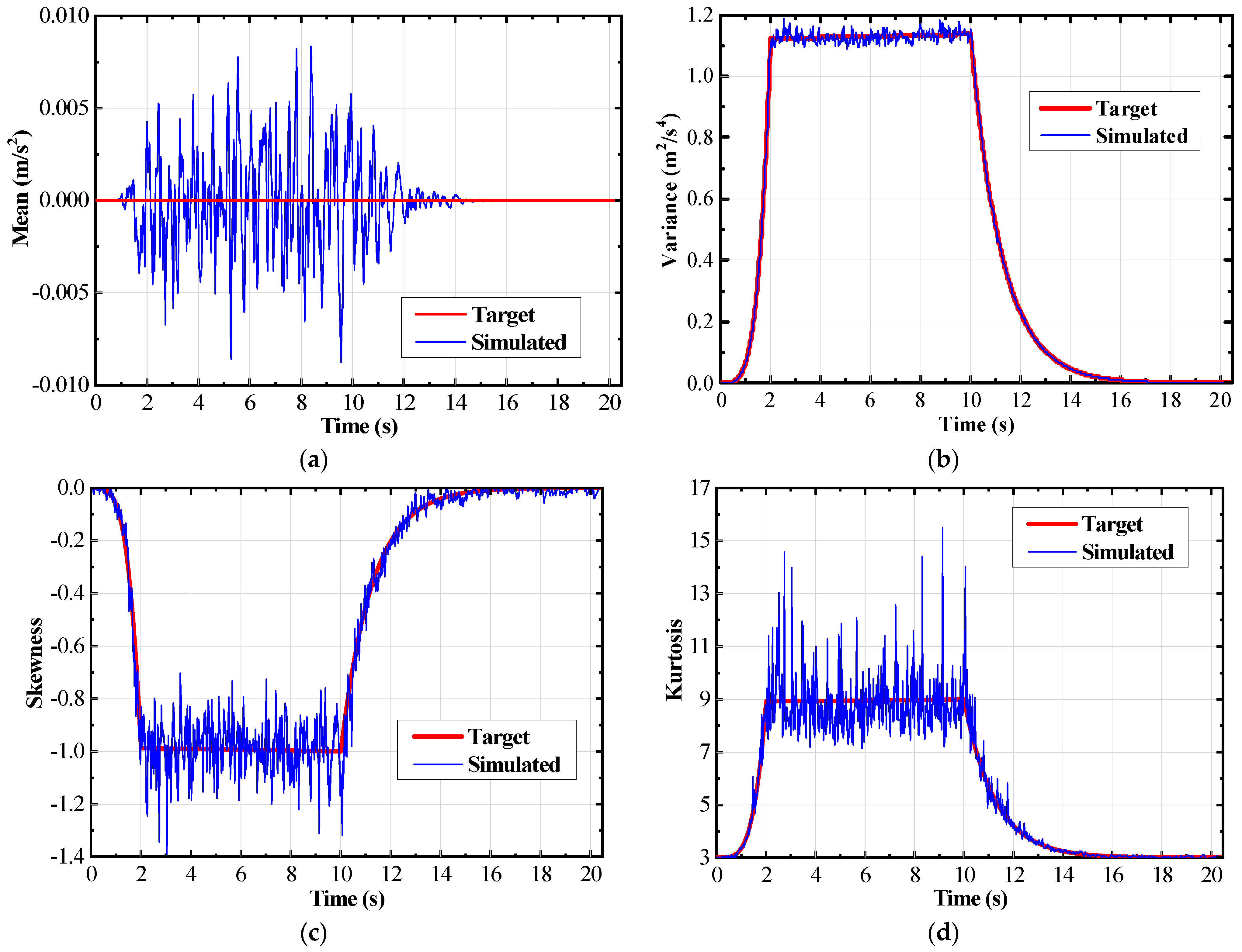
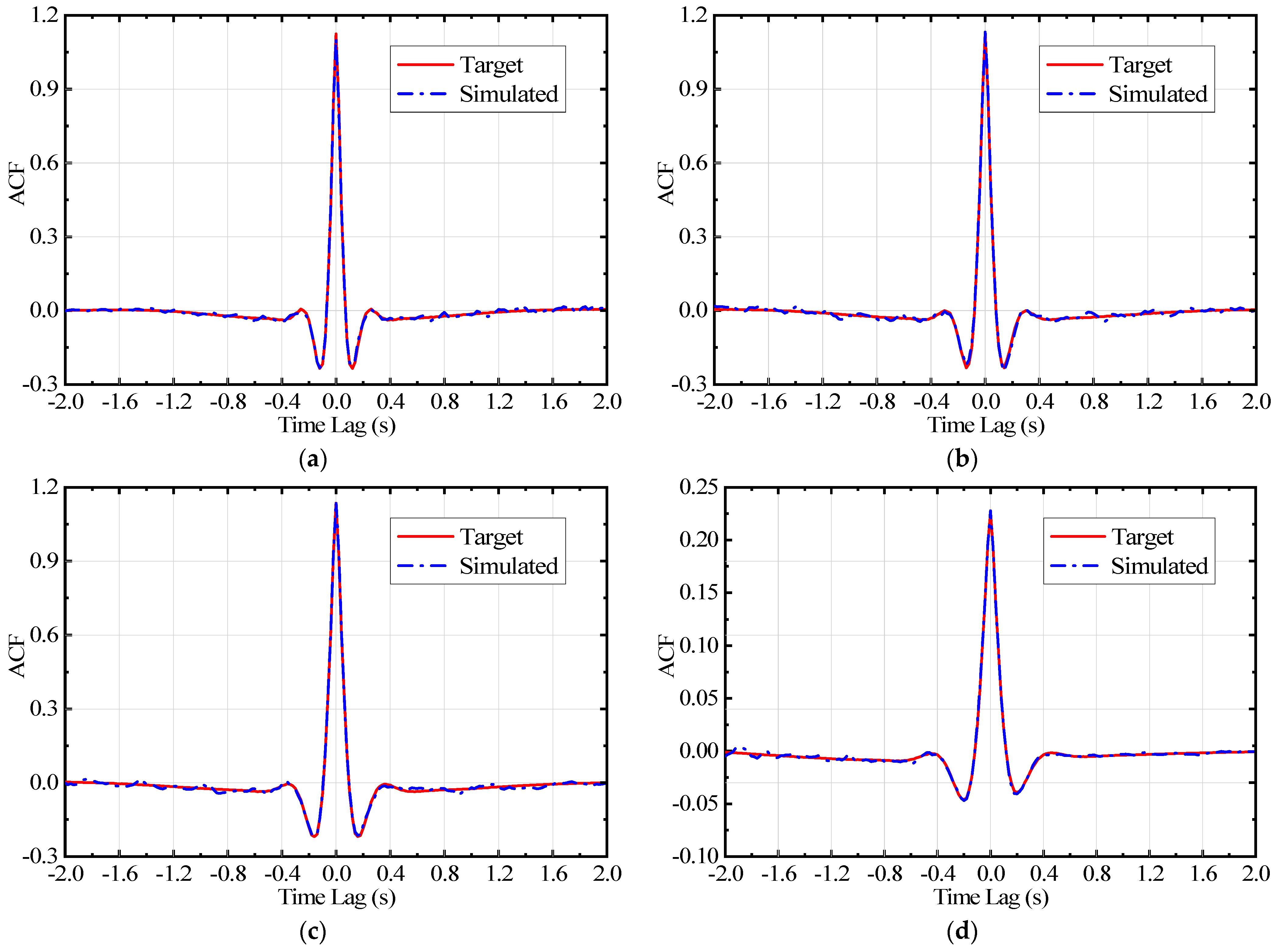
2.2. Generation of Non-Gaussian Non-Stationary Ground Motions

The target EPSD of ground acceleration used herein was also applied in references [1,2,39], it is represented as

$$s\left(\omega ,t\right)=M^2\left(t\right)S_0\left(t\right)\underset{\mathrm{Nonstationary} \mathrm{Kanai}\text{-}\mathrm{Tajimi} \mathrm{spectrum}}{\underbrace{\left[{\displaystyle \frac{1+4{\zeta }_g^2{\left(\frac{\omega }{{\omega }_g}\right)}^2}{{\left[1-{\left(\frac{\omega }{{\omega }_g}\right)}^2\right]}^2+4{\zeta }_g^2{\left(\frac{\omega }{{\omega }_g}\right)}^2}}\right]}}\times \underset{\mathrm{Clough}\text{-}\mathrm{Penzien} \mathrm{correction}}{\underbrace{\left[{\displaystyle \frac{{\left(\frac{\omega }{{\omega }_f}\right)}^4}{{\left[1-{\left(\frac{\omega }{{\omega }_f}\right)}^2\right]}^2+4{\zeta }_f^2{\left(\frac{\omega }{{\omega }_f}\right)}^2}}\right]}}$$

(9a)

$$M\left(t\right)=\left\{\begin{array}{c}{\left(\mathrm{t}/t_1\right)}^2\\ 1\\ e^{-\lambda \left(t-t_2\right)}\end{array}\right.\begin{array}{c}0\le t\le t_1\\ t_1\le t\le t_2\\ t\ge t_2\end{array}$$

(9b)

$$S_0\left(t\right)={\displaystyle \frac{{\sigma }^2}{\pi {\omega }_g\left(\frac{1}{2{\zeta }_g}+2{\zeta }_g\right)}}$$

(9c)

where ${\omega }_g=30-1.25t$ and ${\zeta }_g=0.5+0.005t$ are characteristic frequency and damping of the ground soil, respectively; ${\omega }_f=0.1{\omega }_g$ and ${\zeta }_f={\zeta }_g$ are filtering parameters of the Clough–Penzien correction; other parameters are set as: $\sigma =1.1 \left({\mathrm{m}/\mathrm{s}}^{3/2}\right)$, $t_1=2$ s, $t_2=10$ s, and $\lambda =0.4$. The simulation was performed over a duration of 20.48 s, employing a sampling frequency of 50 Hz. Following the recommended approach, a TVAR model order of 100 was applied. The time-varying target skewness (SK) and kurtosis (KU) were determined as follows:

$$SK\left(t\right)={\displaystyle \frac{-Var\left(t\right)}{\max \left[Var\left(t\right)\right]}}$$

(10a)

$$KU\left(t\right)=6\left|SK\left(t\right)\right|+3$$

(10b)

where $Var\left(t\right)$ denotes the time-varying target variance, which is dependent on the desired EPSD.

A total of 20,000 non-Gaussian ground acceleration time histories were generated. An illustrative example is presented in Figure 1. It can be observed that the negative skewness results in significant negative-going impulses. Figure 2 illustrates the comparisons of the first four-order time-varying moments between the generated samples and the target values. Figure 3, on the other hand, displays the comparisons of the NACF at specific time instants of 3 s, 6 s, 9 s, and 12 s. The chosen model order of 100 yields optimal fitting between the time range of −2 s to 2 s, due to the sampling frequency of 50 Hz. The good agreements in the comparisons affirm the accuracy and reliability of the generated samples in relation to the desired targets.

3. Numerical Examples

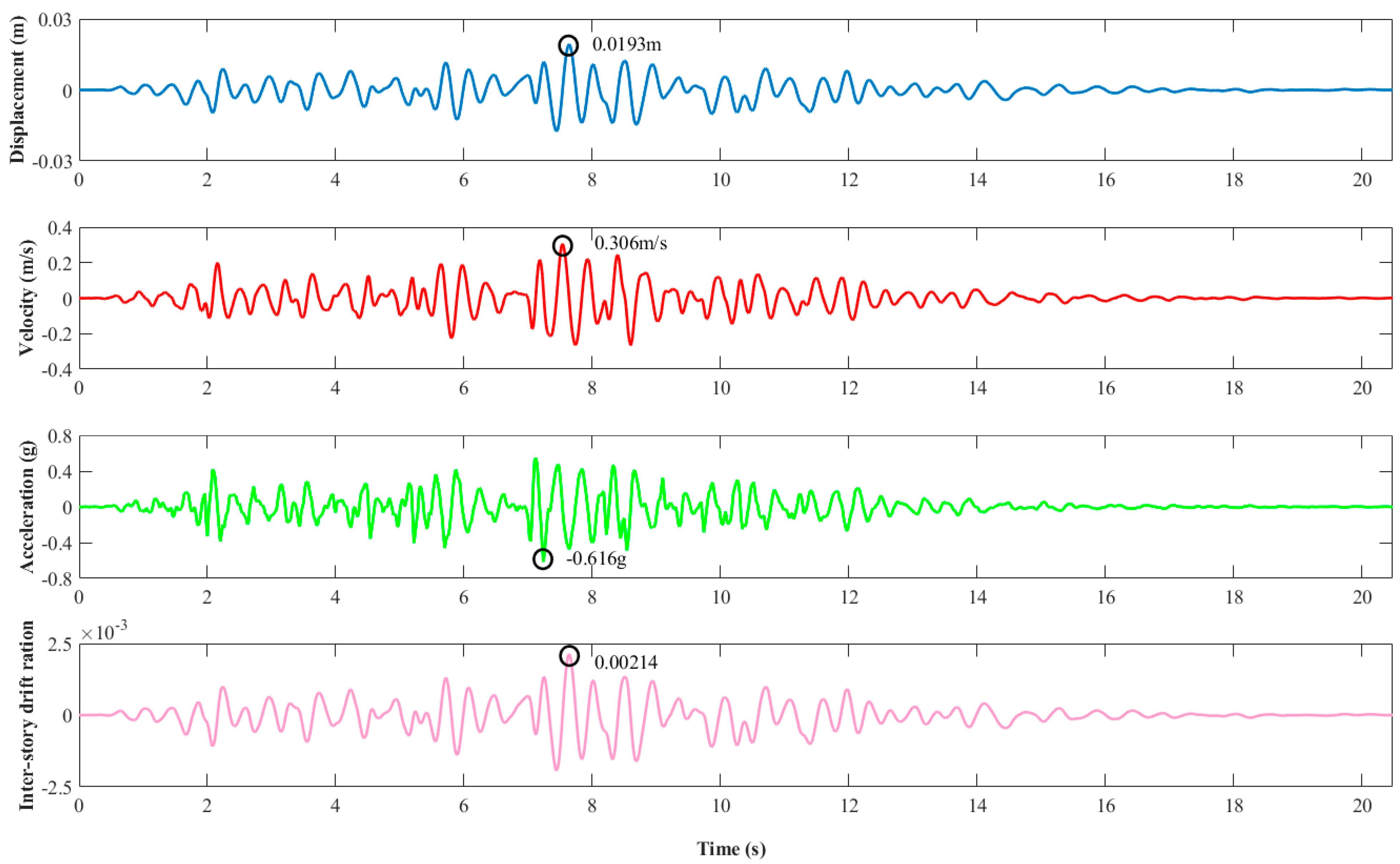
3.1. Multi-Story Frame Structure

There is a four-story reinforced concrete frame building. The height of the first floor is 3.5 m, and the other floors are each 3 m high. Due to the significantly higher stiffness of the floor plan compared to the lateral stiffness between floors, it can be considered that the structure primarily experiences horizontal lateral displacements during seismic events. Consequently, the structure can be simplified as a multi-mass system. The mass of each floor is calculated as half the sum of the masses of the adjacent floors. These masses are then concentrated at the elevation of each floor in the frame structure, creating a four-degree-of-freedom system, as illustrated in Figure 4. A viscoelastic damper is installed on each floor. The main parameters of the structure and dampers are listed in

Table 1. Information about the frame structure.

Structural Parameters	Floor Number
	1	2	3	4
Interlayer mass (×105) (kg)	m1 = 6	m2 = 5	m3 = 5	m4 = 5
Structural interlayer stiffness (×108) (N/m)	k1 = 6	k2 = 5	k3 = 5	k4 = 4
Layer height (m)	h1 = 3.5	h2 = 3	h3 = 3	h4 = 3
Damper stiffness (×108) (N/m)	kd1 = 0.7	kd2 = 0.7	kd3 = 0.7	kd4 = 0.7
Damping of dampers (×106) (N·s/m)	cd1 = 6.8	cd2 = 6.8	cd3 = 6.8	cd4 = 6.8

.

The dynamic equation for this frame structure is represented as

$$M_0\ddot{X}+C_0\dot{X}+K_{0}X+R=-M_{0}I {\ddot{x}}_g$$

(11)

where $X={\left[x_1,x_2,x_3,x_4\right]}^T$ is the horizontal displacement of each floor in the frame structure; $I={\left[1,1,1,1\right]}^T$ is a unit vector; ${\ddot{x}}_g$ is the seismic acceleration; $M_0$, $C_0$, and $K_0$ denote the matrices for mass, damping, and stiffness of the frame structure, respectively; Rayleigh damping is adopted in this case, and its formula is $C_0=a{M}_0+b{K}_0$, where $a=\xi \omega$, $b={\displaystyle \raisebox{1ex}{$\xi $}\!\left/ \!\raisebox{-1ex}{$\omega $}\right.}$. The damping ratio $\xi$ is set to 0.05, taking into account the characteristics of concrete structures. $\omega$ represents the circular frequency of the first-order vibration mode for this frame structure, and its value is 13.6 rad/s in this case. The force exerted by the dampers on the structure, denoted as R, is calculated as $R=C_1\dot{X}+K_{1}X$, where $C_1$ and $K_1$ are expressed as follows:

$$C_1=\left[\begin{array}{cccc}{c}_{d1}+c_{d2}& -c_{d2}& & \\ c_{d2}& c_{d2}+c_{d3}& -c_{d3}& \\ & -c_{d3}& c_{d3}+c_{d4}& -c_{d4}\\ & & -c_{d4}& c_{d4}\end{array}\right]$$

(12a)

$$K_1=\left[\begin{array}{cccc}{k}_{d1}+k_{d2}& -k_{d2}& & \\ k_{d2}& k_{d2}+k_{d3}& -k_{d3}& \\ & -k_{d3}& k_{d3}+k_{d4}& -k_{d4}\\ & & -k_{d4}& k_{d4}\end{array}\right]$$

(12b)

In this case, two groups of seismic excitations are utilized. The first group comprises 20,000 non-Gaussian ground motion records generated as described in Section 2.2. The second group consists of 20,000 Gaussian ground motion records, also generated by the method introduced in Section 2.2, serving as the comparative group with an identical EPSD to that of the first group. These Gaussian ground motions also possess non-stationary features and share the same EPSD as the non-Gaussian group, as shown in Equation (9). The difference lies in the fact that the third- and fourth-order statistics of the Gaussian group are time-invariant, being 0 and 3, respectively. Assuming zero initial velocity and displacement of the structure, the two groups of ground motions (40,000 records in total) are sequentially applied to the structure. Although 40,000 signals represent a notable quantity, it is still not enough to express the complete characteristics of the ground motion, given its inherently stochastic process nature. The dynamic time history analysis is performed using the Newmark-β method on the MATLAB R2019a platform.

Under the seismic excitation shown in Figure 1, the time history of the displacement, velocity, and acceleration on the top floor is illustrated in Figure 5. The peak displacement at the top of the structure is less than 2 cm. Among the four floors, the second floor exhibits the largest inter-story drift ratio, and its time history plot is displayed at the bottom of Figure 5. The peak inter-story drift ratio is measured as 0.00214 in this case, which is below the limit specified by the Chinese Seismic Design Code [40] of 1/550. This indicates that the structure remains within the elastic deformation range throughout this seismic event, and almost no damage is caused to the structure by this ground motion.

Under the excitation of two groups of simulated ground motions, a total of 40,000 seismic responses were obtained, with 20,000 for each group. The vibration circulates around the original position, resulting in zero mean values for displacement, velocity, acceleration, and inter-story drift ratio responses. The strength of the vibration can be quantified using the standard deviation of the responses. The time-varying standard deviations of the four seismic responses mentioned above were calculated and plotted in Figure 6.

It can be observed that the standard deviations of the four seismic responses vary with time and reach their peaks around 10 s, highlighting the non-stationary nature of the seismic excitation. As for displacement, velocity, and acceleration responses, their time-varying standard deviations increase with the height of the structure, indicating larger variations in amplitude for higher floors during seismic events. However, the inter-story drift ratio exhibits a different trend, with the maximum time-varying standard deviation occurring at the second floor and the minimum at the top floor. As a statistical measure, there is little difference in the standard deviation of structural response for the Gaussian and non-Gaussian ground motions. The results from both groups show a remarkable similarity, with the curves nearly overlapping. This is because, for the same structure, the standard deviation of the response is a second-order statistic that is solely related to the second-order statistics of the input ground motion. Since both groups of ground motions have the same EPSD, their second-order statistics are expected to be similar as well.

Traditional seismic probabilistic analysis assumes the seismic motion to be a Gaussian non-stationary process, focusing solely on the second-order statistics of the response. However, in this regard, there is no distinction between Gaussian and non-Gaussian ground motions. Therefore, to investigate the influence of non-Gaussianity on the seismic performance of structures, further attention is needed to the higher-order statistics. The time-varying skewness and kurtosis of displacement, velocity, acceleration, and inter-story drift ratio were calculated, as illustrated in Figure 7 and Figure 8. An analysis of these figures reveals the following findings: (1) The structural response induced by Gaussian ground motion consistently adheres to a Gaussian distribution, characterized by skewness values near zero and kurtosis values close to three. (2) The structural response resulting from non-Gaussian seismic motion still retains the non-Gaussian characteristics, though it exhibits an evident moderation in non-Gaussianity compared to the input ground motion. The skewness values are small, with peaks around 0.2, indicating that the response curves are almost symmetric. On the other hand, the kurtosis values are relatively large, exceeding four, signifying the presence of significant amplitude impulses in the response. The seismic response PDF at the time instant when the peak kurtosis occurs was fitted and plotted in Figure 9, accompanied by a Gaussian PDF curve with the same mean and standard deviation for comparative purposes. Apparently, the structural response PDF induced by Gaussian ground motion aligns with the Gaussian distribution. Conversely, the PDF of the structural response resulting from non-Gaussian ground motion exhibits discernible deviations, characterized by sharper peaks and a heightened concentration towards the center.

The non-Gaussian feature of the structural response, as depicted in Figure 7, Figure 8 and Figure 9, has a significant impact on the extreme values of the response. Displacement and inter-story drift ratio are usually two key damage indicators with specific limit requirements in seismic design codes. Consequently, by extracting the maximum amplitudes from the time histories of displacement on the top floor and inter-story drift ratio on the second floor, extreme response PDF and cumulative distribution function (CDF) curves were, respectively, fitted using the kernel smoothing method and the empirical CDF method. The results were plotted in Figure 10 and Figure 11. Distinct differences between the extreme value distribution curves of Gaussian and non-Gaussian structural responses can be observed. The non-Gaussian extreme distribution displays a longer tail, indicating a higher probability of the appearance of large extreme responses. Previous research indicated that the extreme values of structural seismic responses adhere to a logarithmic normal distribution [6]. Therefore, Figure 10 also displays the fitting outcomes from the lognormal distribution. In Figure 10, the results from the present study are labeled as “kernel” or “empirical”. They are obtained from data-based and non-parametric methods and can thus serve as benchmarks. The results from the lognormal distribution, labeled as “lognormal”, align well with our results. This convergence not only supports the validity of using the lognormal distribution to model the extremes of structural seismic responses but also attests to the reliability of the results obtained in this research. Additionally, the methods employed in this paper, namely the kernel smoothing method and the empirical CDF method, are grounded in non-parametric data models and serve as benchmark references. These methods offer a robust comparative framework for the analysis.

The mean values, as well as the response extrema corresponding to the crossing probabilities of 75%, 85%, and 95%, are listed in

Table 2. Extreme values of Gaussian and non-Gaussian responses for the frame structure.

	Displacement (cm)				Inter-Story Drift Ratio (×10−3)
	Mean	75%	85%	95%	Mean	75%	85%	95%
Gaussian	3.23	3.54	3.81	4.25	3.63	3.98	4.27	4.77
Non-Gaussian	3.42	3.86	4.24	5.02	3.86	4.35	4.78	5.66
Increase ratio	6.99%	9.04%	11.29%	18.12%	7.32%	9.30%	11.94%	18.66%

for comparison. Additionally, the increase ratios of non-Gaussian extremes relative to Gaussian extremes were computed and included at the bottom of Table 2. Evidently, the average values of extreme displacement and inter-story drift ratio under the influence of non-Gaussian seismic excitation are approximately 7% higher. Moreover, for the same crossing probabilities, the extreme values of non-Gaussian responses surpass those of Gaussian responses, with a larger disparity as the crossing probability increases.

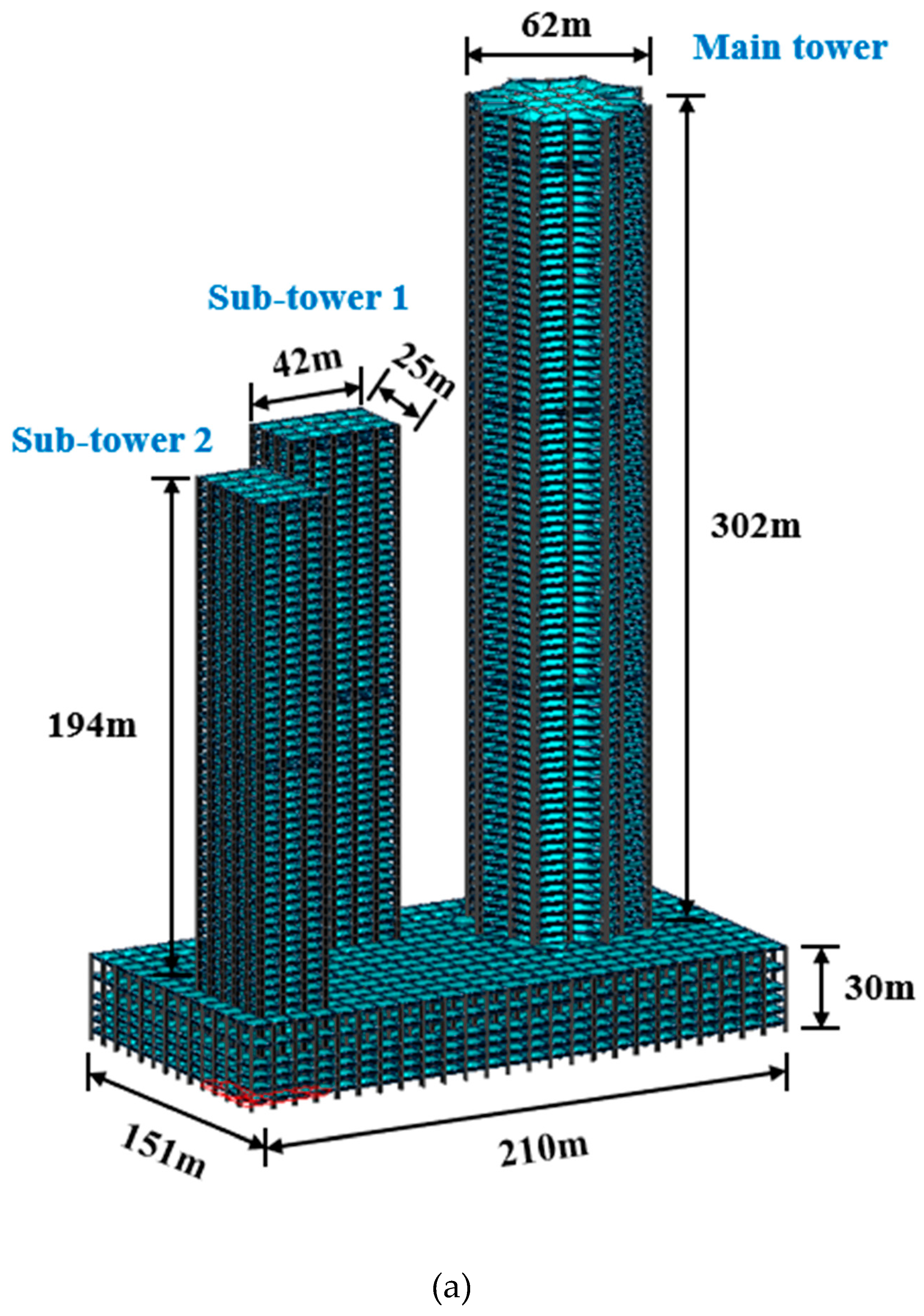
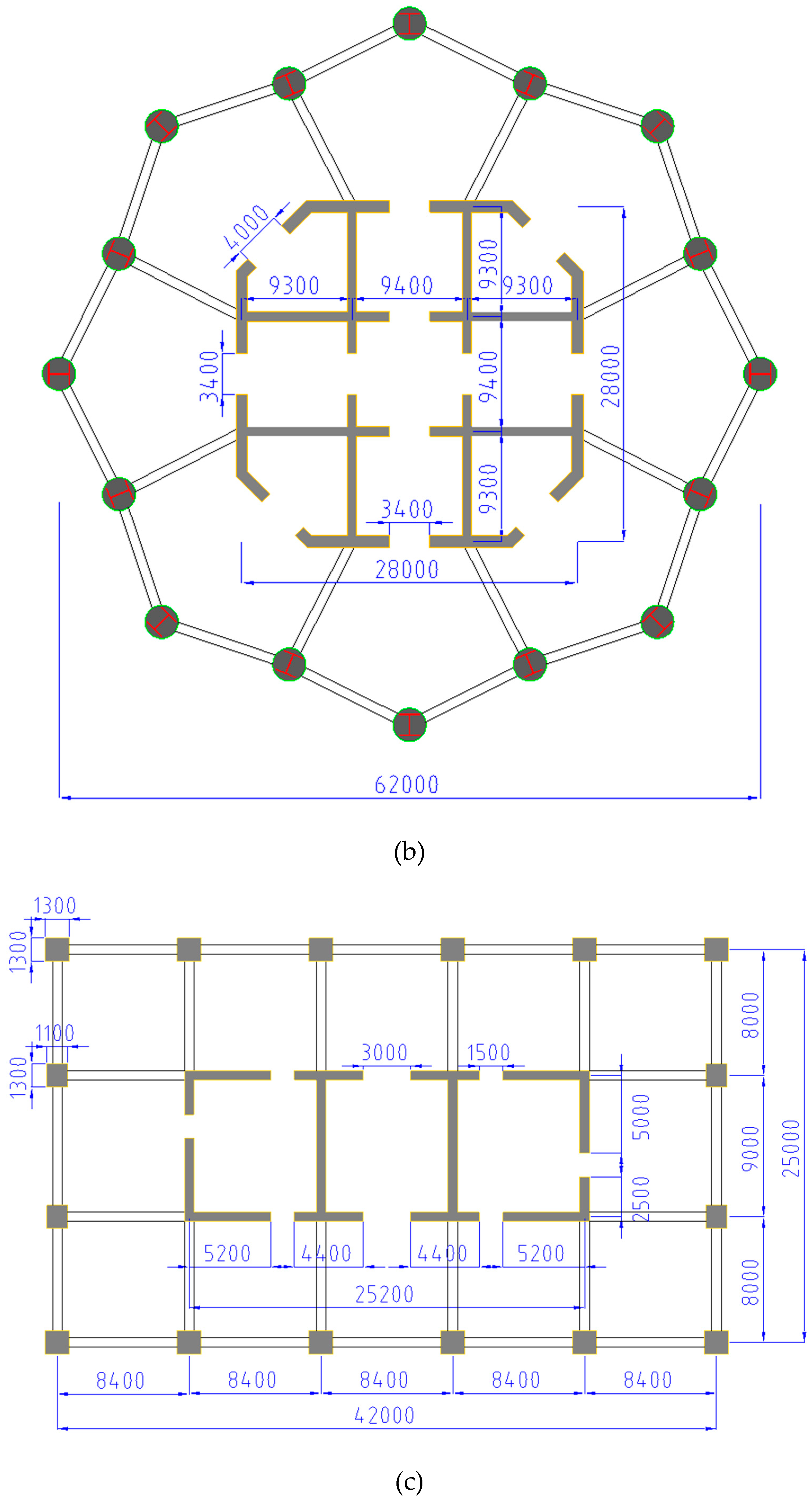
3.2. Multi-Tower High-Rise Building

In this section, we aim to investigate the impact of non-Gaussian characteristics in ground motion on the seismic performance of a complex building. A case study is conducted on a super high-rise commercial center located in Sichuan Province, China. The selected building comprises a main tower and two sub-towers, all interconnected by a large plate at the bottom measuring 210 m × 151 m × 30 m, as depicted in Figure 12. The main tower is an 82-story structure reaching a height of 302 m. Each of the two sub-towers comprises 52 stories with a height of 194 m. The distance between the main tower and the closer sub-tower measures 30 m. The distances between the two sub-towers in both the north–south and east–west directions are 25 m.

The main tower consists of a reinforced concrete core tube, an outer frame, and an outrigger truss. The dimensions of the core tube are 28 m × 28 m, with a wing wall thickness ranging from 1.0 m at the bottom to 0.6 m at the top. The concrete used in the core tube has a grade of C50. The outer frame is constructed using steel columns and frame beams. Outrigger trusses are positioned around the 27th, 54th, and 78th floors, serving as connections between the steel columns, core tube, and external outrigger steel trusses. All metallic elements are fabricated from Q345 steel. The two sub-towers have an identical structural form of frame–core tube. The reinforced concrete core tube in each sub-tower measures 25 m × 9 m, with a uniform wall thickness of 0.6 m. The concrete grade employed for the core tube construction is C50.

The finite element analysis software Midas Building was used for dynamic analysis in this study. Column elements were used to simulate frame columns. Giant frame column elements were used to simulate external frames with steel columns. Beam elements were used to model frame beams, and core wall elements for shear walls. To facilitate efficient dynamic calculations, the computational model was simplified by utilizing rigid plates to represent the floor slabs, and the effects of pile–soil interaction were not taken into account. Rayleigh damping was employed with a damping ratio of 0.045.

The first 30 modal shapes of the structure were derived using modal analysis conducted through the Lanczos method, a widely used technique for extracting eigenvalues and eigenvectors. For ease of reference, the direction parallel to the long side of the bottom plate is designated as the X-direction, while its perpendicular direction is denoted as the Y-direction. The sub-tower closer to the main tower is named Sub-tower 1. The first six vibration modes of the structure are shown in

Table 3. The first six vibration modes of the structure.

Mode Order	Frequency (Hz)	Period (s)	Main Tower	Sub-Tower 1	Sub-Tower 2
1	0.14	7.03	First-order translation	/	/
2	0.19	5.38	/	Translation in Y-direction	Translation in X-direction
3	0.29	3.41	/	Translation in X-direction	Translation in Y-direction
4	0.54	1.86	/	First-order torsion	First-order torsion
5	0.56	1.79	First-order torsion	/	/
6	0.72	1.39	Second-order translation	/	/

.

The first-order mode primarily encompasses the translation of the main tower, while exhibiting minimal vibrations in the two sub-towers. As a result, their vibration modes are not explicitly presented. In the second-order mode, Sub-tower 1 demonstrates Y-directional translation, whereas Sub-tower 2 displays X-directional translation. The third-order mode involves the X-directional translation of Sub-tower 1 and the Y-directional translation of Sub-tower 2. In the fourth-order mode, the sub-tower experiences first-order torsion, with the ratio of its first-order torsion period to the first-order translation period being 0.35. The fifth-order mode corresponds to torsion in the main tower, with the ratio of its first-order torsion period to translation period measuring 0.25.

Given the computational demands and time constraints associated with the complex finite element analysis, a limited number of simulations were conducted for this case study. Specifically, 200 simulations were performed, including 100 scenarios with non-Gaussian seismic excitation and 100 scenarios with Gaussian seismic excitation. The seismic input signals were sourced from the artificial seismic signals used in Section 3.1. Out of the 40,000 available records, 100 non-Gaussian seismic motions and 100 Gaussian seismic motions were randomly selected. Each selection was inputted into the Y-direction of the structure. The maximum inter-story drift angle of the main tower was observed around the 70th floor. These values were extracted, in addition to the maximum displacement responses at the top floor. Subsequently, the PDFs and CDFs of these extreme values were fitted and portrayed in Figure 13 and Figure 14. The CDF curves were estimated using the empirical CDF method. Due to the limited number of extreme value samples available for both the Gaussian and non-Gaussian groups, amounting to only 100 samples in each group, the resulting CDF curves are relatively coarse. It is evident that the tail of the distribution of structural responses caused by non-Gaussian ground motion is longer, indicating that even if the EPSD is the same, non-Gaussian ground motions are more likely to cause extreme damage to the structure compared to Gaussian ground motions. Furthermore, the mean values, as well as the response extrema corresponding to the crossing probabilities of 75%, 85%, and 95%, are listed in

Table 4. Extreme values of Gaussian and non-Gaussian responses for the main tower.

	Displacement (cm)				Inter-Story Drift Ratio (×10−3)
	Mean	75%	85%	95%	Mean	75%	85%	95%
Gaussian	45.1	54.3	60.3	72.1	2.33	2.76	3.01	3.51
Non-Gaussian	46.1	56.3	64.5	79.9	2.40	2.85	3.22	3.95
Increase ratio	2.17%	3.64%	6.87%	11.01%	3.16%	3.55%	6.74%	12.51%

for comparison. According to Table 4, it can be observed that under various crossing probabilities, the extreme structural responses induced by non-Gaussian ground motions are consistently higher than those induced by Gaussian ground motions. Moreover, as the crossing probability increases, the increase ratio of the structural responses also correspondingly expands.

It should be emphasized that the findings presented in this section are based solely on two buildings. Their global applicability will be further examined in future work. The authors believe that similar phenomena would likely be observed in buildings with different designs and characteristics.

4. Conclusions

This paper investigated the influence of non-Gaussianity in ground motions on the seismic performance of buildings. It filled a significant gap in the structural engineering literature by considering ground motion as a non-Gaussian process, which is often overlooked in traditional seismic analysis. By employing a non-Gaussian non-stationary random process simulation method proposed by the authors, 40,000 ground motion acceleration signals were efficiently generated, including 20,000 Gaussian and 20,000 non-Gaussian records. A four-story frame building and a three-tower super-tall building were selected as computational examples. The generated acceleration signals were used as external excitations for the two buildings. The purpose was to compare the differences in seismic responses caused by the Gaussian and non-Gaussian earthquake groups. Probability analysis was performed using top-layer displacement and maximum inter-story drift ratio as damage indicators. The comparative analysis yields the following findings:

(a)

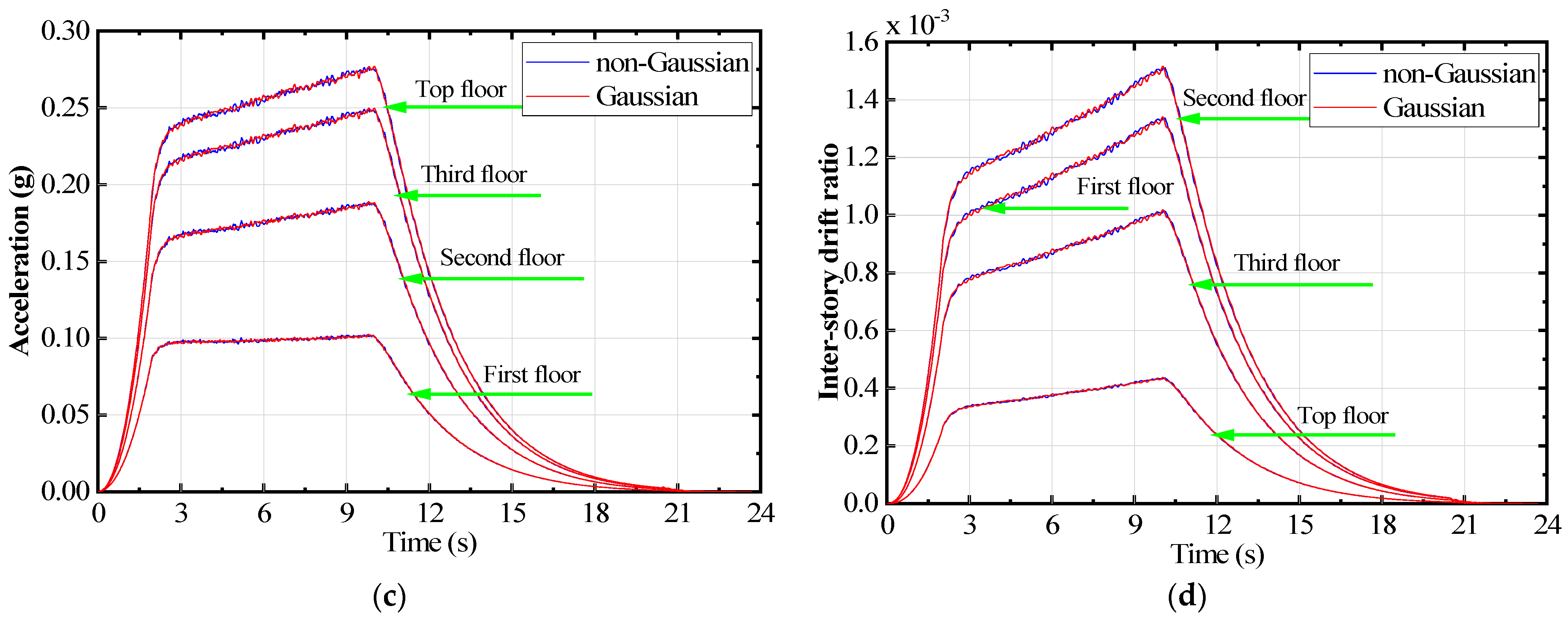
The structural responses induced by both Gaussian and non-Gaussian earthquake groups, such as displacement, velocity, acceleration, and inter-story drift ratio, have identical first- and second-order moments, namely mean and standard deviation.

(b)

The higher-order moments of the structural responses caused by the two earthquake groups differ evidently. The responses of Gaussian earthquakes remain Gaussian; the responses of non-Gaussian earthquakes exhibit prominent non-Gaussian features, although the non-Gaussian strength is relatively weakened compared to the external excitation.

(c)

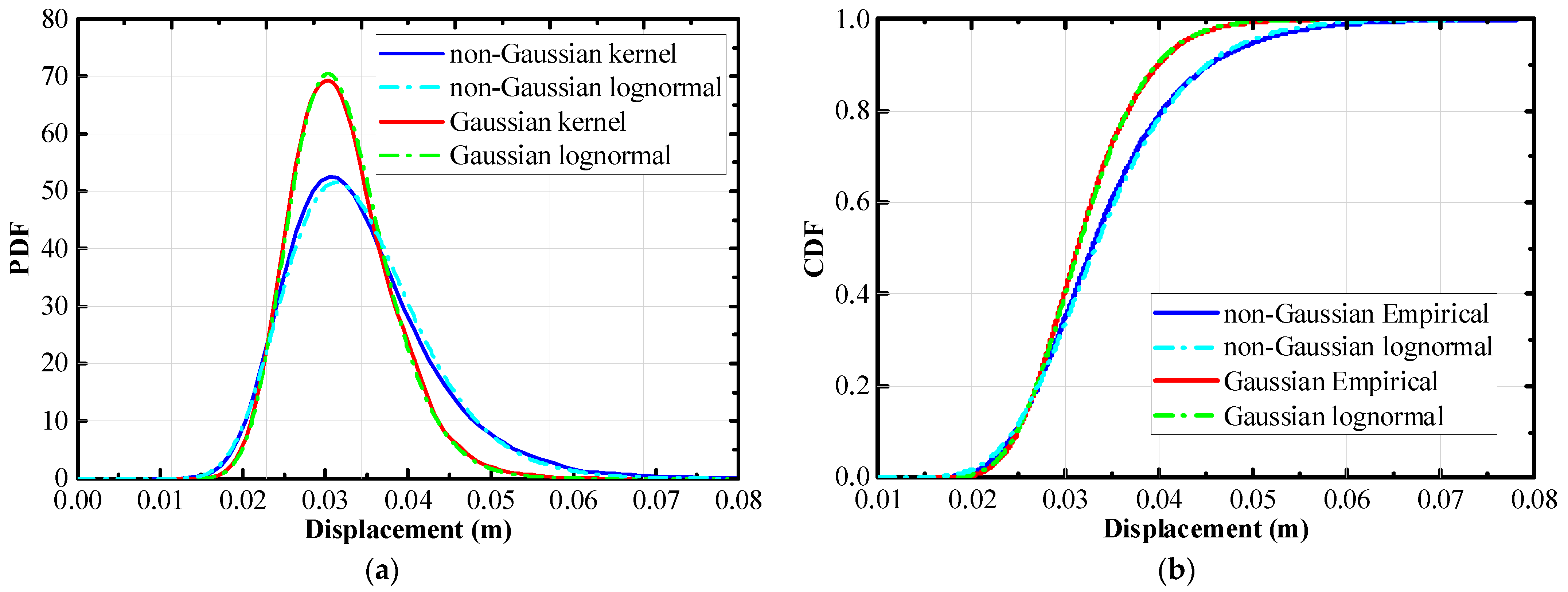
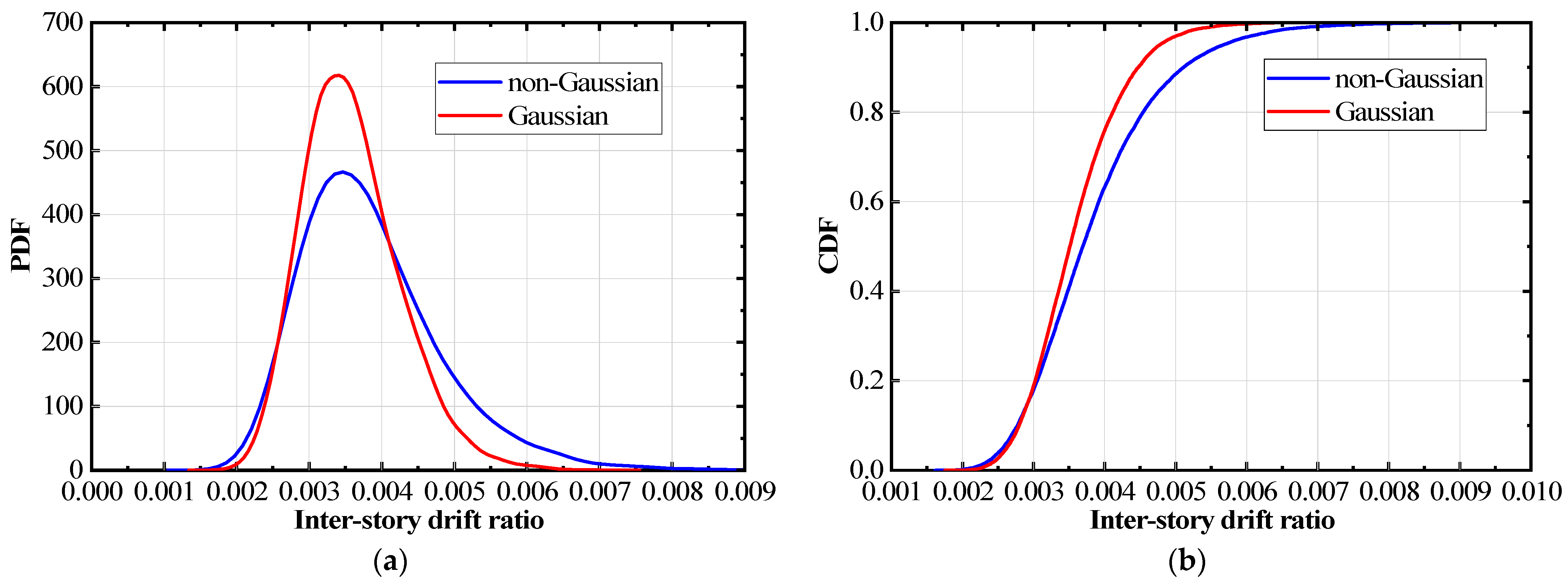
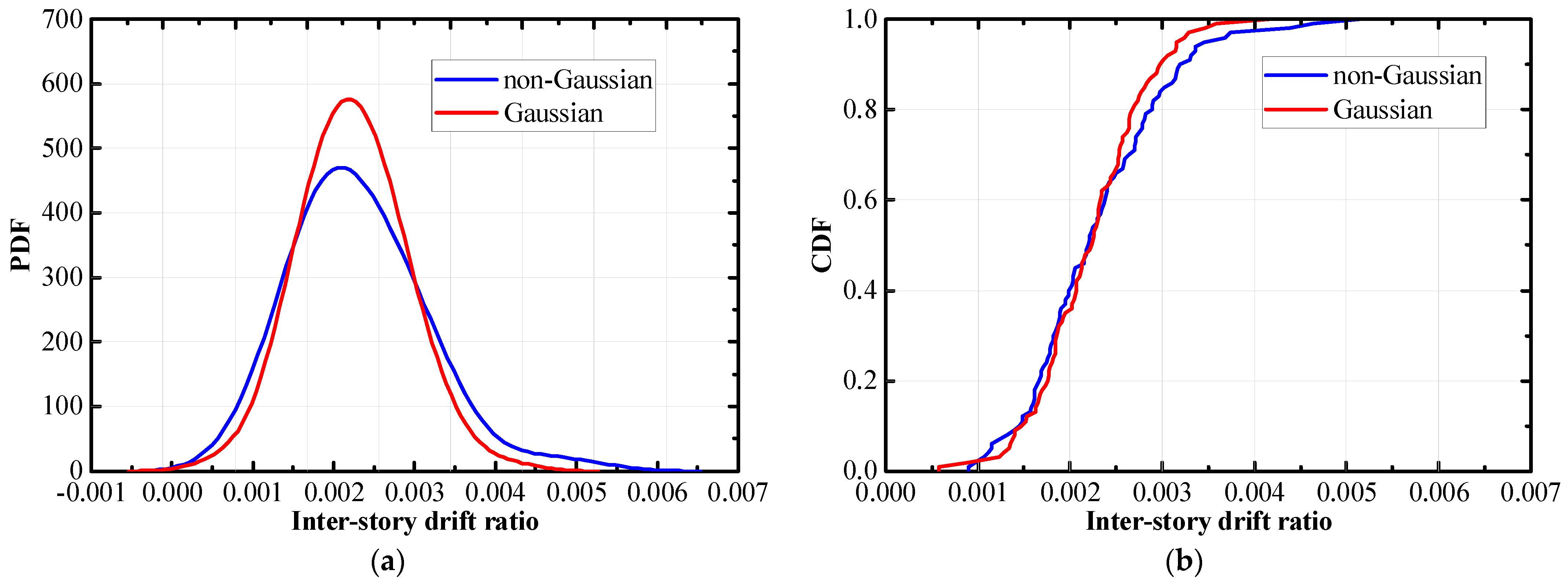
Due to the influence of non-Gaussianity, the probability density functions of the two groups of structural responses at any given time show significant differences.

(d)

The analysis of extreme values reveals that the tail of non-Gaussian structural response distribution is longer than that of the Gaussian counterpart. This results in a significantly larger value of non-Gaussian responses under high crossing probabilities, with an amplification that can exceed 18%.

(e)

Non-Gaussianity exhibits a significant amplifying effect on the seismic response of structures, which should be taken into account in seismic design.

References

1. Wu, Y.; Gao, Y.; Zhang, N.; Zhang, F. Simulation of spatially varying non-Gaussian and nonstationary seismic ground motions by the spectral representation method. ASCE J. Eng. Mech. 2018, 144, 04017143. [Google Scholar] [CrossRef]
2. Xu, F.; Ma, X. An efficient simulation algorithm for non-gaussian nonstationary processes. Probabilistic Eng. Mech. 2021, 63, 103105. [Google Scholar] [CrossRef]
3. Gusev, A.A. Peak factors of Mexican accelerograms: Evidence of a non-gaussian amplitude distribution. J. Geophys. Res. Solid Earth 1996, 101, 20083–20090. [Google Scholar] [CrossRef]
4. Kafali, G.; Grigoriu, M. Non-Gaussian model for spatially coherent seismic ground motions. In Application of Statistics and Probability in Civil Engineering; Der Kiureghian, A., Madanat, P., Eds.; Millpress: Rotterdam, The Netherlands, 2003. [Google Scholar]
5. Zentner, I.; Poirion, F. Enrichment of seismic ground motion databases using Karhunen–Loéve expansion. Earthq. Eng. Struct. Dyn. 2012, 41, 1945–1957. [Google Scholar] [CrossRef]
6. Romao, X.; Delgado, R.; Costa, A. Assessment of the statistical distributions of structural demand under earthquake loading. J. Earthq. Eng. 2011, 15, 724–753. [Google Scholar] [CrossRef]
7. Liu, Z.; Li, X.; Zhang, Z. Quantitative identification of near-fault ground motions based on ensemble empirical mode decomposition. KSCE J. Civ. Eng. 2020, 24, 922–930. [Google Scholar] [CrossRef]
8. Cheng, Y.; Dong, Y.R.; Bai, G.L.; Wang, Y.Y. IDA-based seismic fragility of high-rise frame-core tube structure subjected to multi-dimensional long-period ground motions. J. Build. Eng. 2021, 43, 102917. [Google Scholar] [CrossRef]
9. Ansari, M.; Nazari, M.; Panah, A.K. Influence of foundation flexibility on seismic fragility of reinforced concrete high-rise building. Soil Dyn. Earthq. Eng. 2021, 142, 106521. [Google Scholar] [CrossRef]
10. Guo, W.; Guo, L.; Zhai, Z.; Li, S. Seismic performance assessment of a super high-rise twin-tower structure connected with rotational friction negative stiffness damper and lead rubber bearing. Soil Dyn. Earthq. Eng. 2022, 152, 107039. [Google Scholar] [CrossRef]
11. He, X.; Xu, C.; Xu, X.; Yang, Y. Advances on the avoidance zone and buffer zone of active faults. Nat. Hazards Res. 2022, 2, 62–74. [Google Scholar] [CrossRef]
12. Liu, Q.; Zhang, W.; Bhatt, M.W.; Kumar, A. Seismic nonlinear vibration control algorithm for high-rise buildings. Nonlinear Eng. 2022, 10, 574–582. [Google Scholar] [CrossRef]
13. Kandemir, E.C.; Mortazavi, A. Optimizing base isolation system parameters using a fuzzy reinforced butterfly optimization: A case study of the 2023 Kahramanmaras earthquake sequence. J. Vib. Control 2024, 30, 502–515. [Google Scholar] [CrossRef]
14. Kandemir, E.C.; Mortazavi, A. Optimization of seismic base isolation system using a fuzzy reinforced swarm intelligence. Adv. Eng. Softw. 2022, 174, 103323. [Google Scholar] [CrossRef]
15. Baker, J.W.; Cornell, C.A. A vector-valued ground motion intensity measure consisting of spectral acceleration and epsilon. Earthq. Eng. Struct. Dyn. 2005, 34, 1193–1217. [Google Scholar] [CrossRef]
16. Hancock, J.; Watson-Lamprey, J.; Abrahamson, N.A.; Bommer, J.J.; Markatis, A.; McCoy, E.; Mendis, R. An improved method of matching response spectra of recorded earthquake ground motion using wavelets. J. Earthq. Eng. 2006, 10, 67–89. [Google Scholar] [CrossRef]
17. Samanta, A.; Pandey, P. Effects of ground motion modification methods and ground motion duration on seismic performance of a 15-storied building. J. Build. Eng. 2018, 15, 14–25. [Google Scholar] [CrossRef]
18. Taheri, S.; Mohammadi, R.K. An enhanced sequential ground motion selection for risk assessment using a Bayesian updating approach. J. Build. Eng. 2022, 46, 103745. [Google Scholar] [CrossRef]
19. Zhu, X.; Broccardo, M.; Sudret, B. Seismic fragility analysis using stochastic polynomial chaos expansions. Probabilistic Eng. Mech. 2023, 72, 103413. [Google Scholar] [CrossRef]
20. Chaudhuri, A.; Chakraborty, S. Reliability of linear structures with parameter uncertainty under non-stationary earthquake. Struct. Saf. 2006, 28, 231–246. [Google Scholar] [CrossRef]
21. Gupta, S.; Manohar, C.S. Reliability analysis of randomly vibrating structures with parameter uncertainties. J. Sound Vib. 2006, 297, 1000–1024. [Google Scholar] [CrossRef]
22. Muscolino, G.; Santoro, R.; Sofi, A. Reliability assessment of structural systems with interval uncertainties under spectrum-compatible seismic excitations. Probabilistic Eng. Mech. 2016, 44, 138–149. [Google Scholar] [CrossRef]
23. Deodatis, G.; Shinozuka, M. Auto-regressive model for nonstationary stochastic processes. ASCE J. Eng. Mech. 1988, 114, 1995–2012. [Google Scholar] [CrossRef]
24. Deodatis, G. Non-stationary stochastic vector processes: Seismic ground motion applications. Probabilistic Eng. Mech. 1996, 11, 149–167. [Google Scholar] [CrossRef]
25. Huang, G.; Liao, H.; Li, M. New formulation of Cholesky decomposition and applications in stochastic simulation. Probabilistic Eng. Mech. 2013, 34, 40–47. [Google Scholar] [CrossRef]
26. Shields, M.D. Simulation of spatially correlated nonstationary response spectrum-compatible ground motion time histories. J. Eng. Mech. 2015, 141, 04014161. [Google Scholar] [CrossRef]
27. Wu, Y.; Gao, Y.; Zhang, L.; Li, D. Simulation of spatially varying ground motions in V-shaped symmetric canyons. J. Earthq. Eng. 2016, 20, 992–1010. [Google Scholar] [CrossRef]
28. Stuart, B.; Ord, J. Kendall’s Advanced Theory of Statistics: Distribution Theory, 6th ed.; Wiley: Hoboken, NJ, USA, 2006. [Google Scholar]
29. Sakamoto, S.; Ghanem, R. Simulation of multi-dimensional non-Gaussian non-stationary random fields. Probabilistic Eng. Mech. 2002, 17, 167–176. [Google Scholar] [CrossRef]
30. Sakamoto, S.; Ghanem, R. Polynomial chaos decomposition for the simulation of non-Gaussian nonstationary stochastic processes. ASCE J. Eng. Mech. 2002, 128, 190–201. [Google Scholar] [CrossRef]
31. Kim, H.; Shields, M. Simulation of Strongly Non-Gaussian Non-Stationary Stochastic Processes Utilizing Karhunen–Loeve Expansion; University of British Columbia: Vancouver, BC, Canada, 2015. [Google Scholar]
32. Shields, M.; Deodatis, G. Estimation of evolutionary spectra for simulation of non-stationary and non-Gaussian stochastic processes. Comput. Struct. 2013, 126, 149–163. [Google Scholar] [CrossRef]
33. Priestley, M. Evolutionary spectra and non-stationary processes. J. R. Stat. Soc. Ser. B 1965, 27, 204–237. [Google Scholar] [CrossRef]
34. Gersch, W.; Kitagawa, G. Time varying AR coefficient model for modelling and simulating earthquake ground motion. Earthq. Eng. Struct. Dyn. 1985, 13, 243–254. [Google Scholar] [CrossRef]
35. Johnson, N.; Kotz, S.; Balakrishnan, N. Continuous Univariate Distributions; Wiley: New York, NY, USA, 1995; Volume 1. [Google Scholar]
36. Winterstein, S. Non-normal responses and fatigue damage. J. Eng. Mech. 1985, 10, 1291–1295. [Google Scholar] [CrossRef]
37. Ma, X.; Xu, F.; Liu, Z. A method for evaluation of the probability density function of white noise filtered non-Gaussian stochastic process. Mech. Syst. Signal Process. 2024, 211, 111242. [Google Scholar] [CrossRef]
38. Ma, X.; Xu, F. Investigation on the sampling distributions of non-Gaussian wind pressure skewness and kurtosis. Mech. Syst. Signal Process. 2024, 220, 111610. [Google Scholar] [CrossRef]
39. Benowitz, B.; Shields, M.; Deodatis, G. Determining evolutionary spectra from non-stationary auto-correlation functions. Probabilistic Eng. Mech. 2015, 41, 73–88. [Google Scholar] [CrossRef]
40. GB 50011-2010; Ministry of Construction of the People’s Republic of China, Code for Seismic Design of Buildings. China Architecture and Building Press: Beijing, China, 2010.
Figure 1. One of the simulated ground accelerations.
Buildings 14 02364 g001
Figure 2. Comparisons between the simulated first four-order time-varying marginal moments and the targets: (a) mean; (b) variance; (c) skewness; (d) kurtosis.
Buildings 14 02364 g002
Figure 3. Comparisons between the simulated ACFs and the targets: (a) t = 3 s; (b) t = 6 s; (c) t = 9 s; (d) t = 12 s.
Buildings 14 02364 g003
Figure 4. Frame structure model.
Buildings 14 02364 g004
Figure 5. Structural seismic response time histories: displacement, velocity, acceleration on the top floor, and inter-story drift ratio on the second floor.
Buildings 14 02364 g005
Figure 6. Time-varying standard deviation of structural seismic response: (a) displacement; (b) velocity; (c) acceleration; (d) inter-story drift ratio.
Buildings 14 02364 g006aBuildings 14 02364 g006b
Figure 7. Time-varying skewness of structural seismic response: (a) displacement on the top floor; (b) velocity on the top floor; (c) acceleration on the top floor; (d) inter-story drift ratio on the second floor.
Buildings 14 02364 g007
Figure 8. Time-varying kurtosis of structural seismic response: (a) displacement on the top floor; (b) velocity on the top floor; (c) acceleration on the top floor; (d) inter-story drift ratio on the second floor.
Buildings 14 02364 g008aBuildings 14 02364 g008b
Figure 9. PDF comparison of structural seismic response at a typical time instant: (a) displacement on the top floor; (b) velocity on the top floor; (c) acceleration on the top floor; (d) inter-story drift ratio on the second floor.
Buildings 14 02364 g009
Figure 10. Comparison of extreme value distribution for displacement on the top floor of the frame structure: (a) PDF; (b) CDF.
Buildings 14 02364 g010
Figure 11. Comparison of extreme value distribution for inter-story drift ratio on the second floor: (a) PDF; (b) CDF.
Buildings 14 02364 g011
Figure 12. Structural model of the three-tower high-rise building: (a) Finite element model; (b) Structural plan for main tower (unit: mm); (c) Structural plan for two sub-towers (unit: mm).
Buildings 14 02364 g012aBuildings 14 02364 g012b
Figure 13. Comparison of extreme value distribution for displacement on the top floor of the main tower: (a) PDF; (b) CDF.
Buildings 14 02364 g013
Figure 14. Comparison of extreme value distribution for inter-story drift ratio on the 70th floor: (a) PDF; (b) CDF.
Buildings 14 02364 g014