
Numerical Study on the Axial Compression Behavior of Composite Columns with High-Strength Concrete-Filled Steel Tube and Honeycombed Steel Web Subjected to Freeze–Thaw Cycles
 ,
,
Abstract
:1. Introduction
2. Analysis Process of the Paper
3. Specimen Design
4. Finite Element Model
4.1. Constitutive Model of Materials
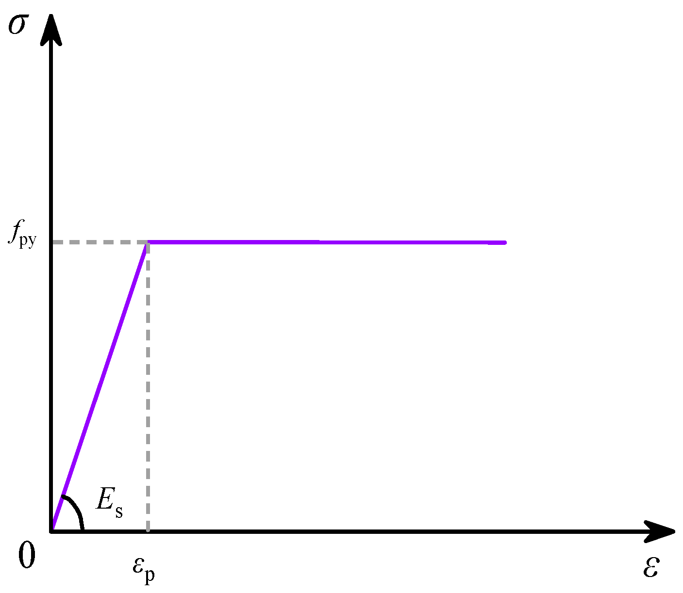
4.1.1. Steel
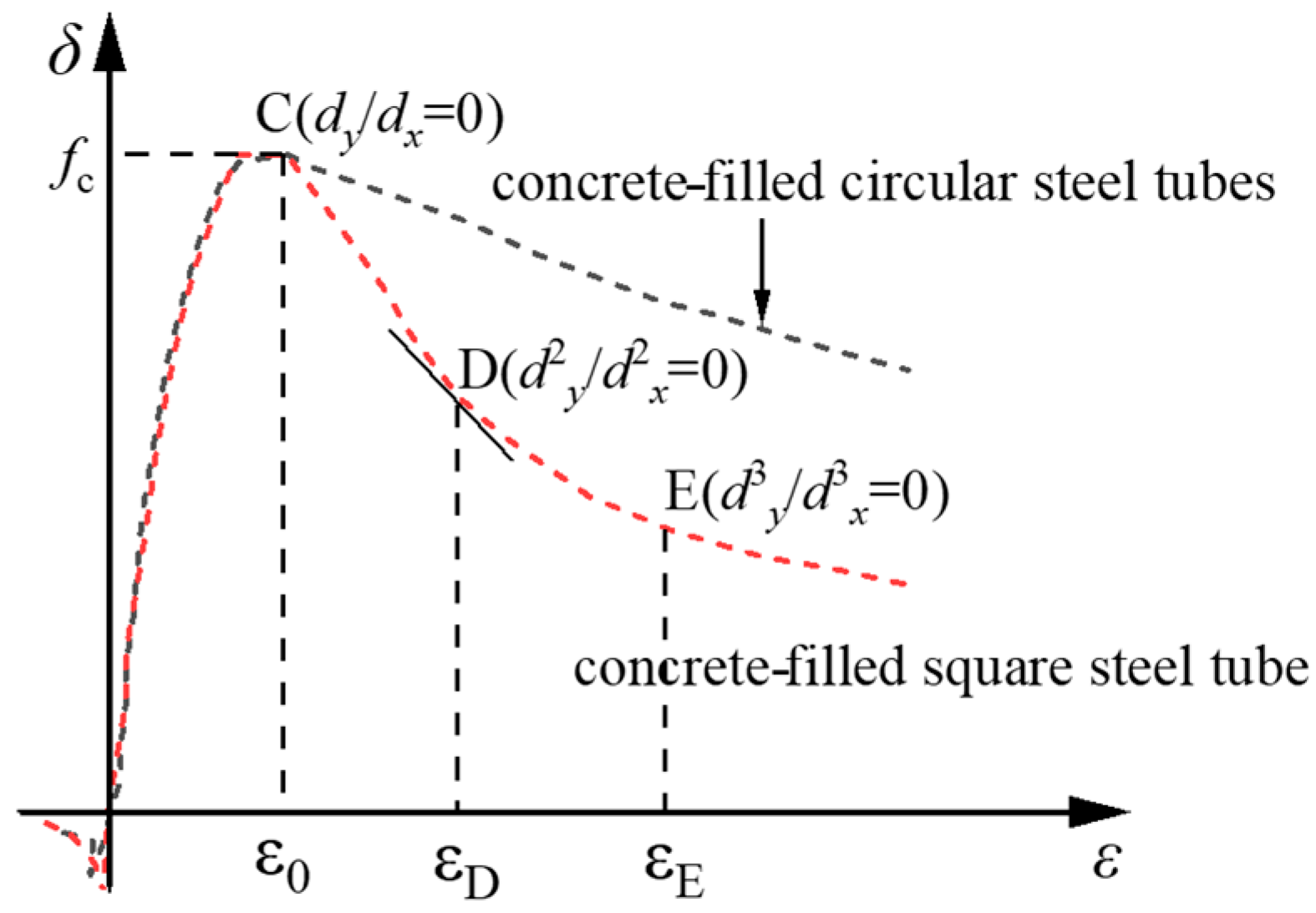
4.1.2. Concrete
4.1.3. Concrete under Freeze–Thaw Cycles
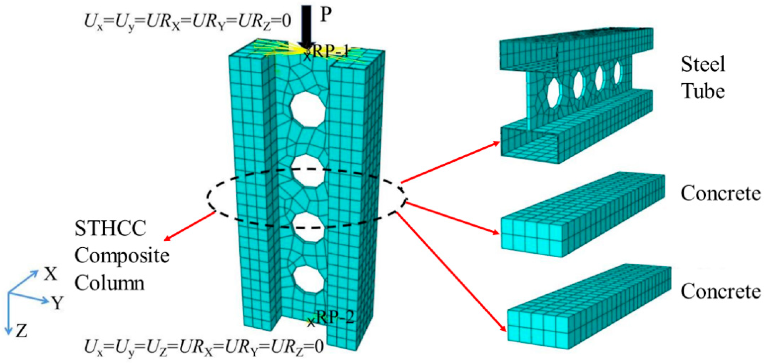
4.2. Establishment of Finite Element Model
4.2.1. Element Type and Contact Method
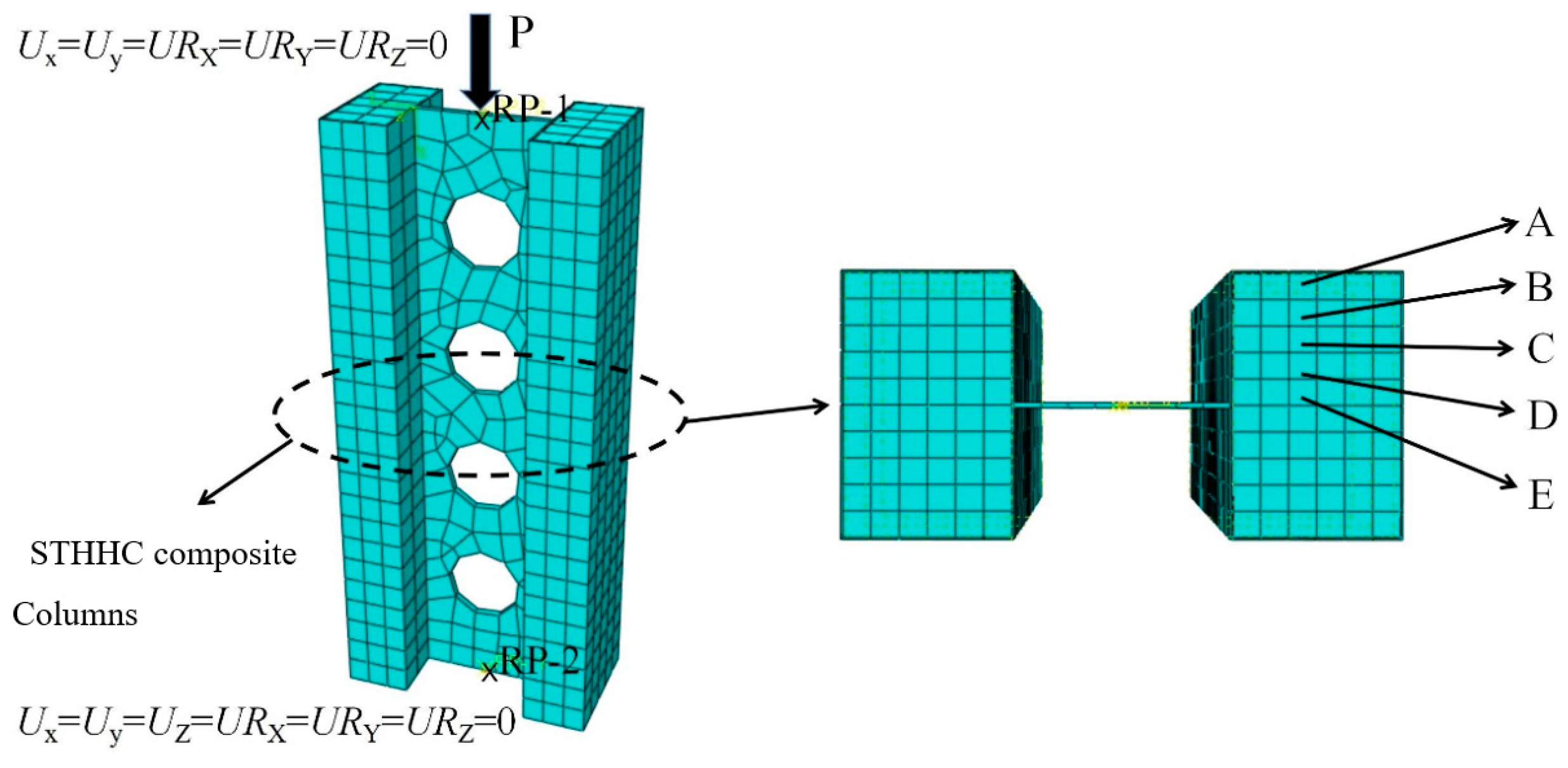
4.2.2. Boundary Conditions and Loading Method
4.2.3. Mesh Division
5. Validation of Finite Element Model
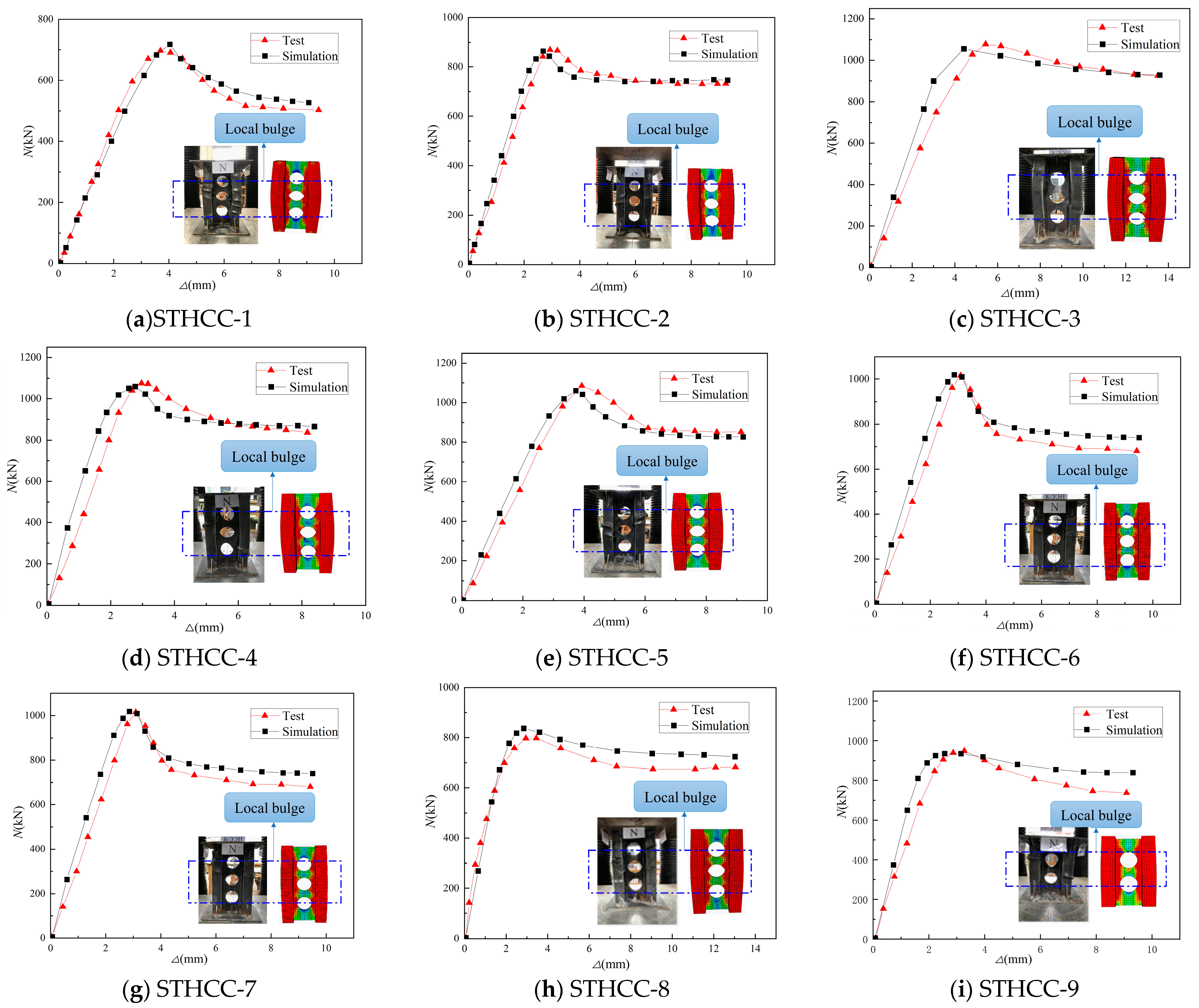
5.1. Validation of Finite Element Model for Concrete-Filled Steel Tube Flange–Honeycomb Steel Web Composite Short Columns
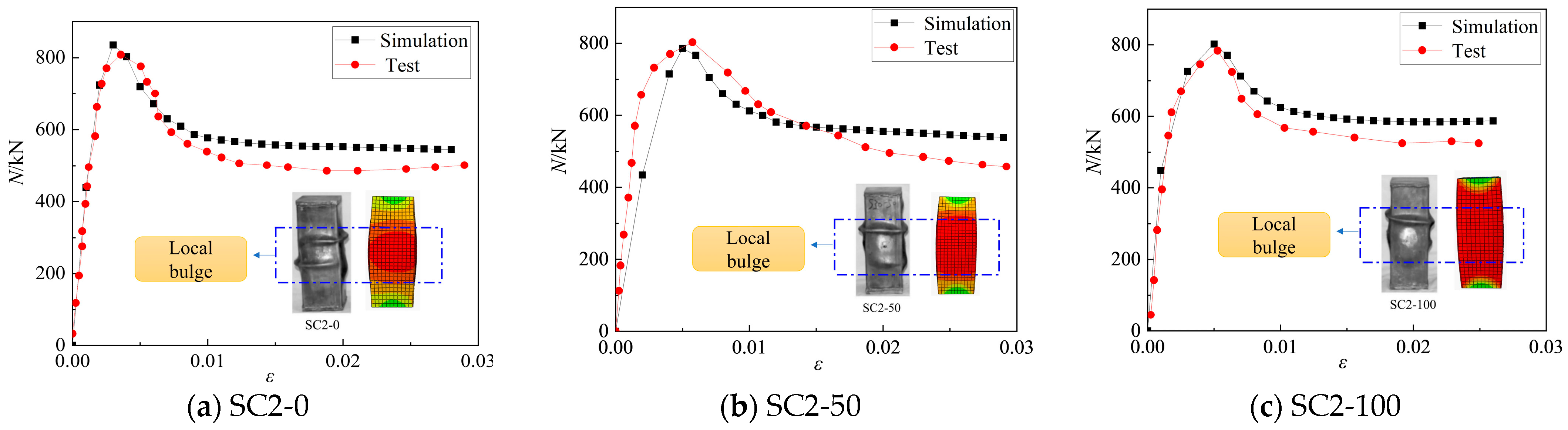
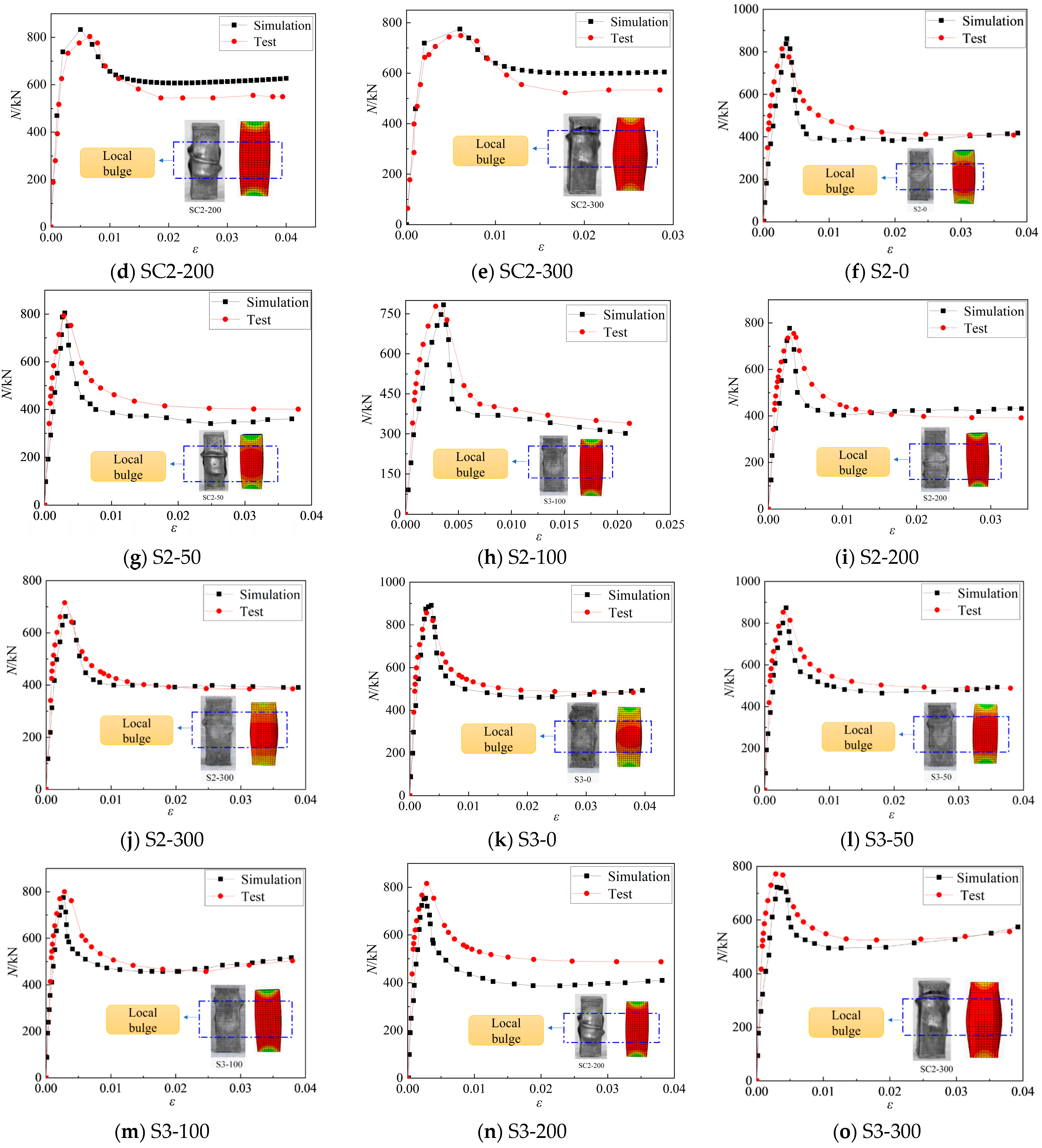
5.2. Validation of Finite Element Model for High-Strength Concrete-Filled Square Steel Tube under Freeze–Thaw Cycles
6. Parametric Analysis
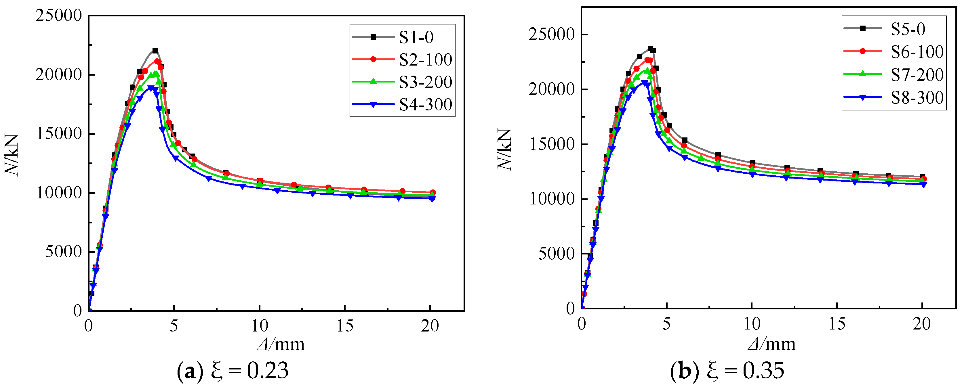
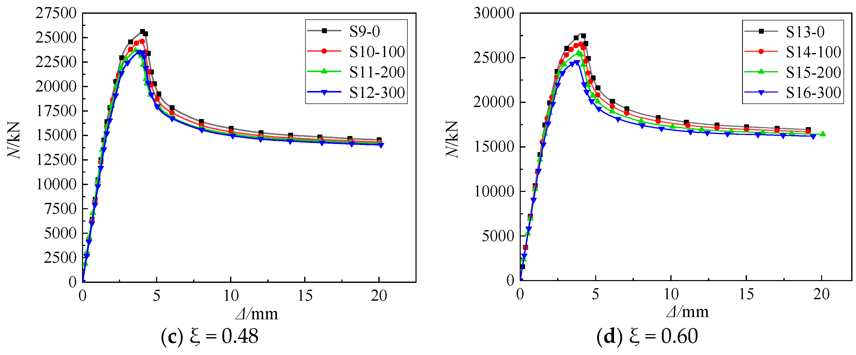
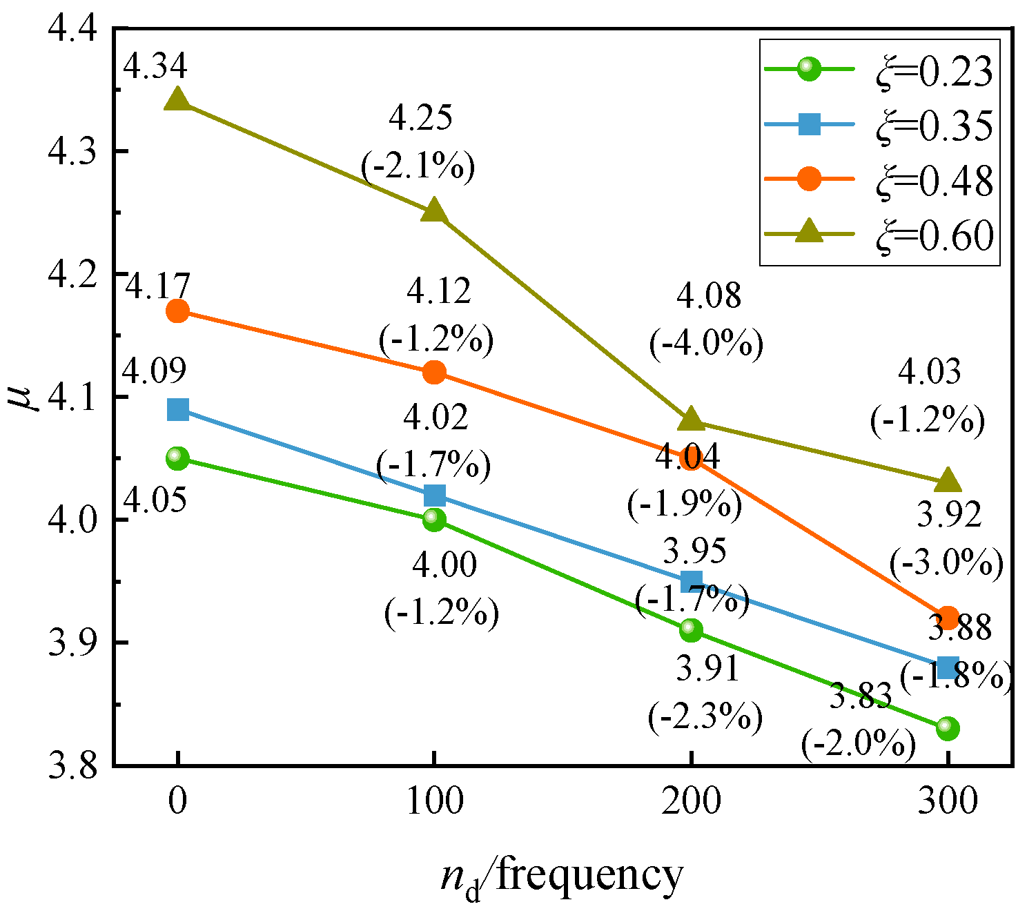
6.1. Confinement Effect Coefficient (ξ)
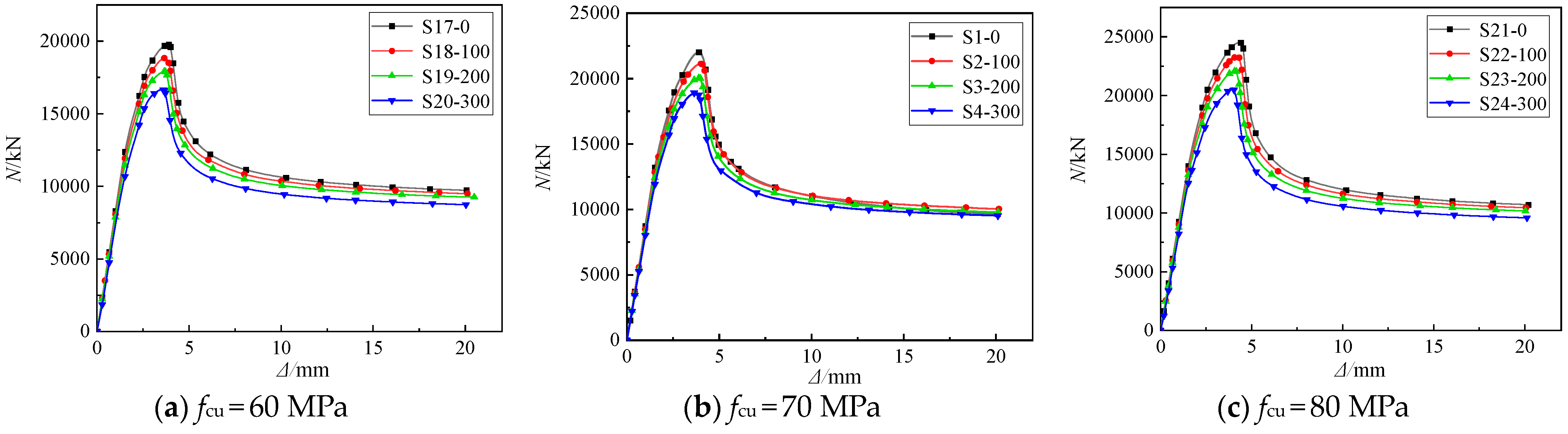
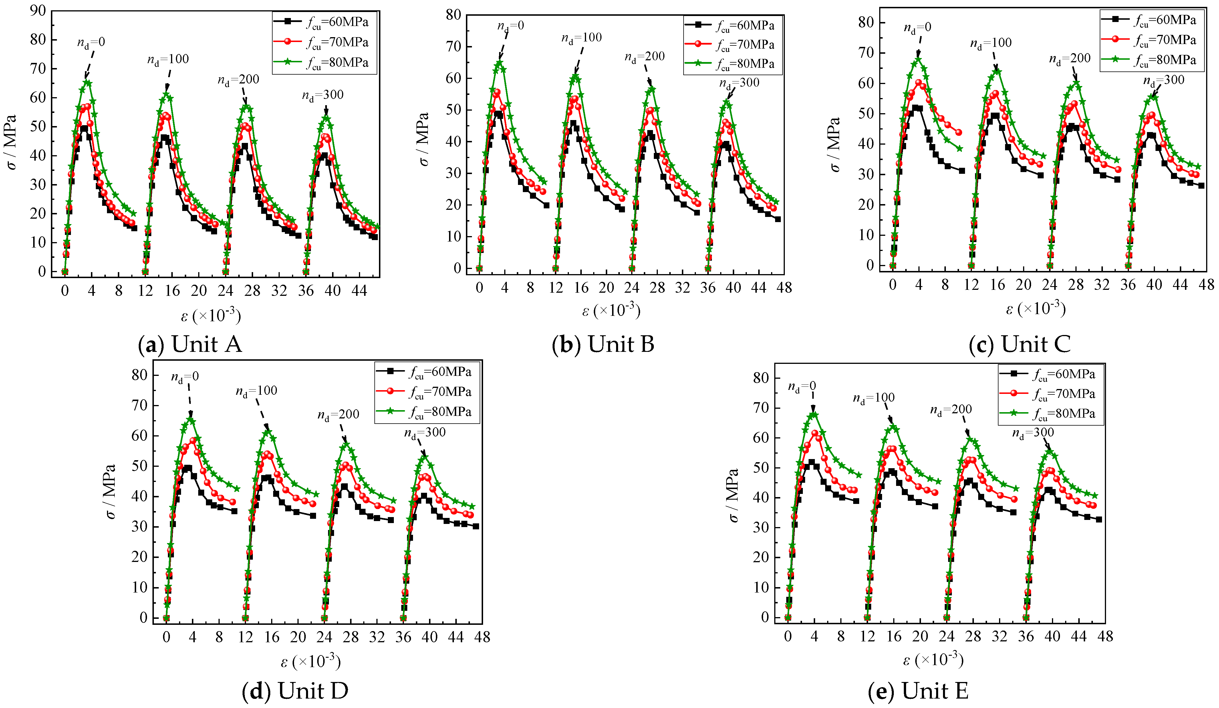
6.2. Cubic Strength of Concrete (fcu)
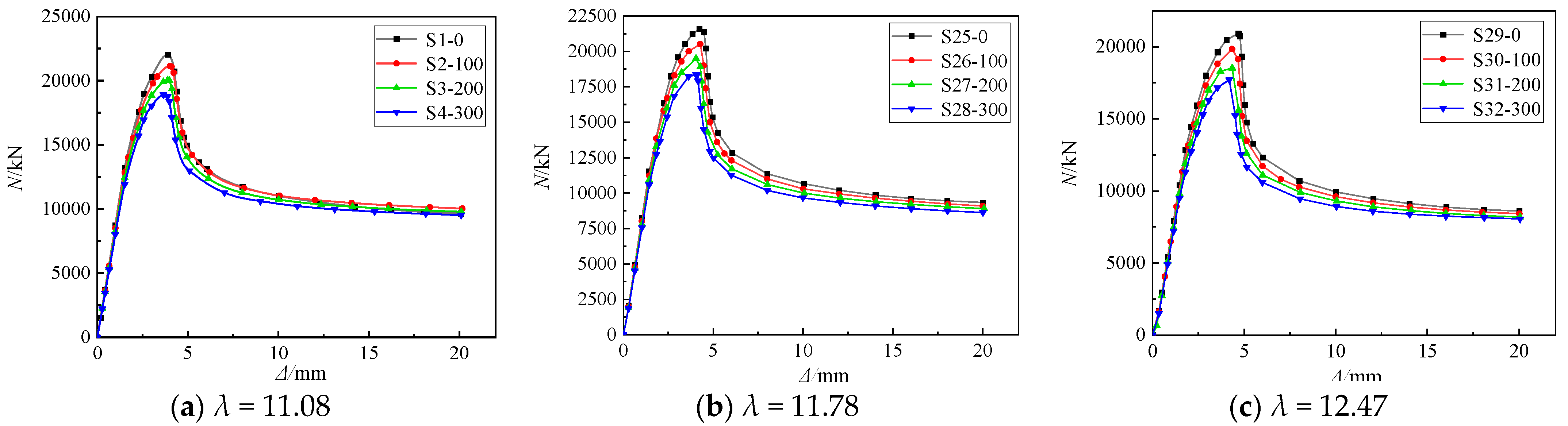
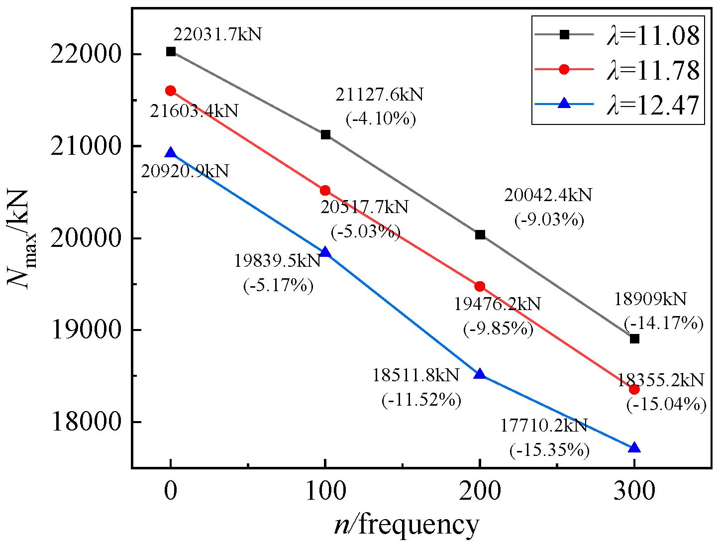
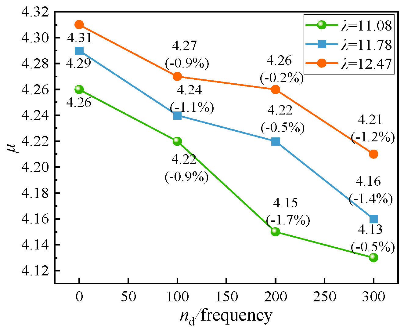
6.3. Slenderness Ratio (λ)
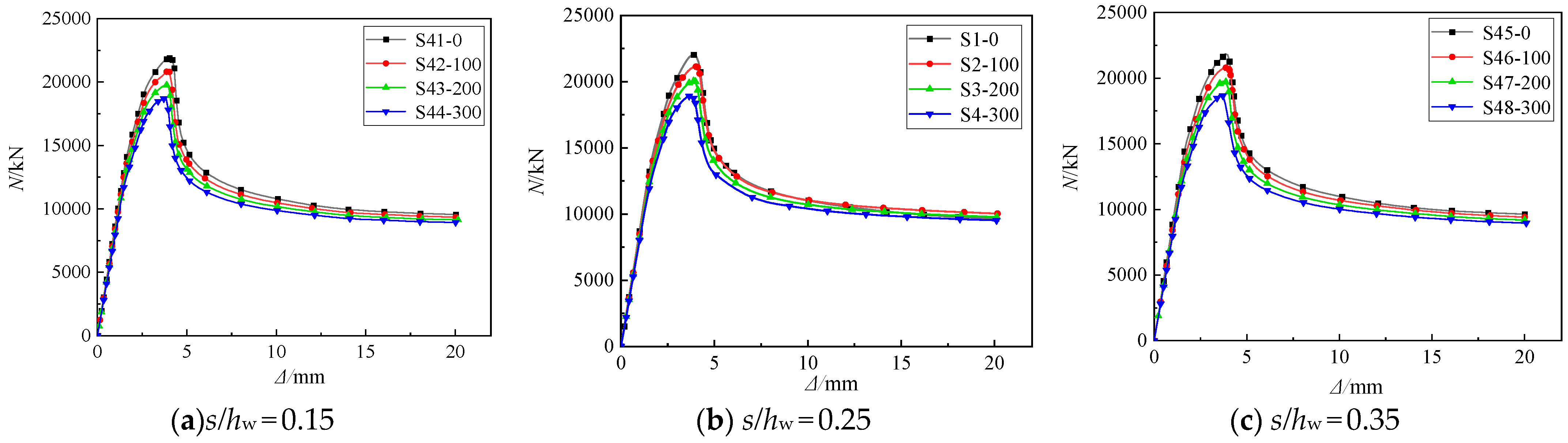
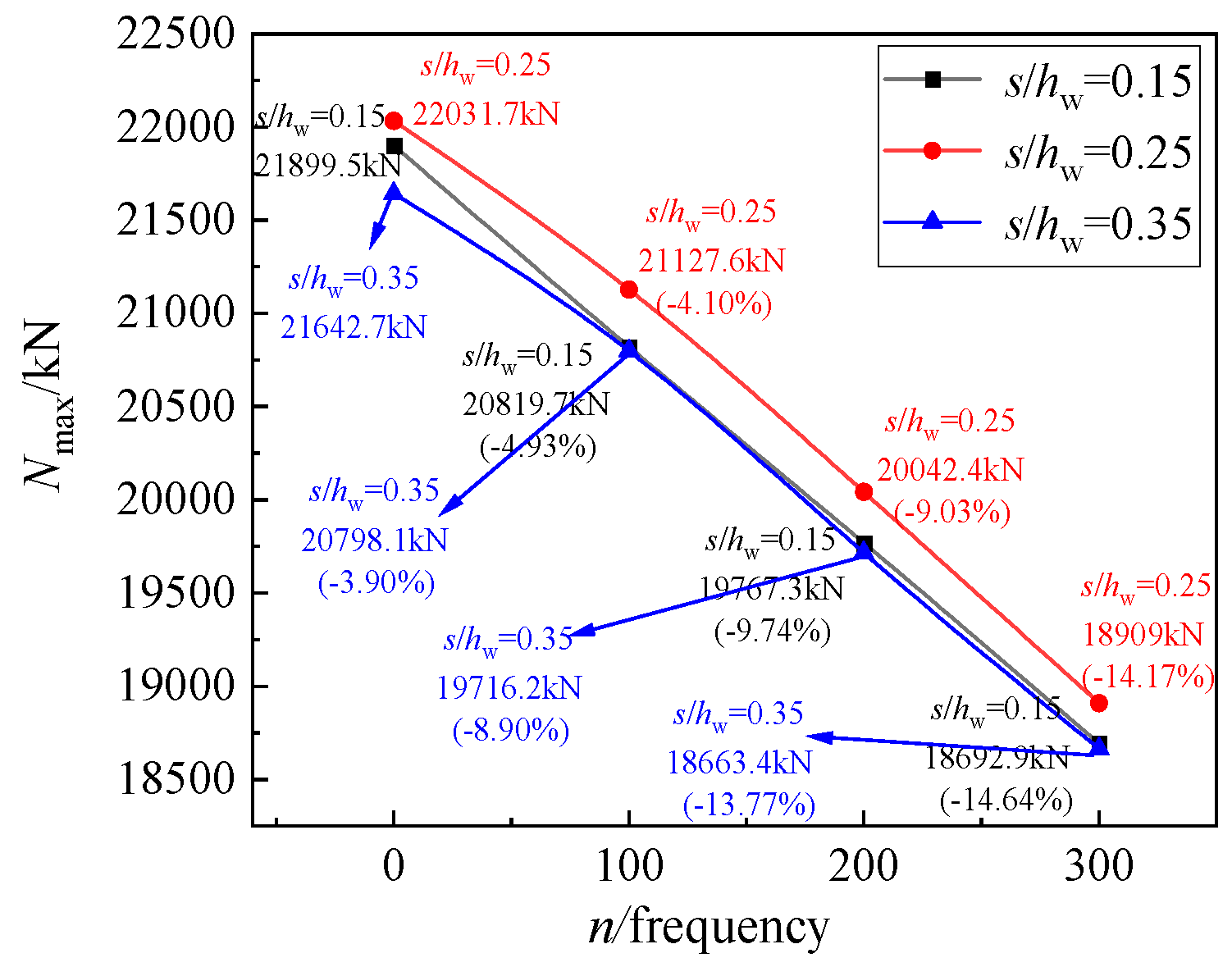
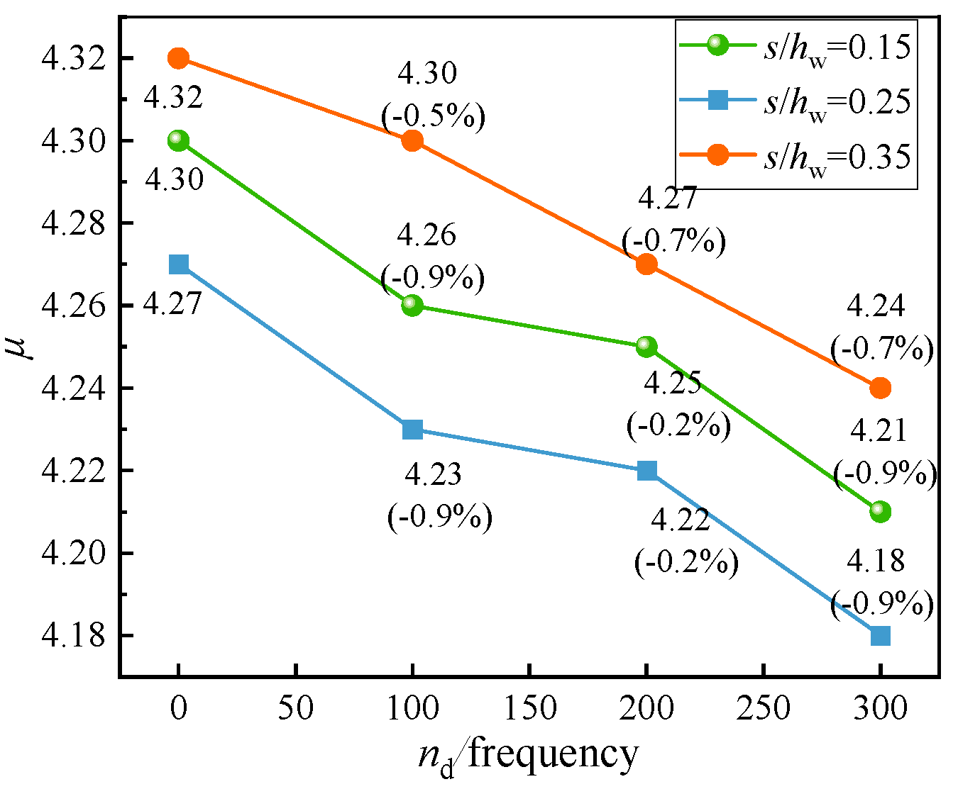
6.4. Aspect Ratio (s/hw)
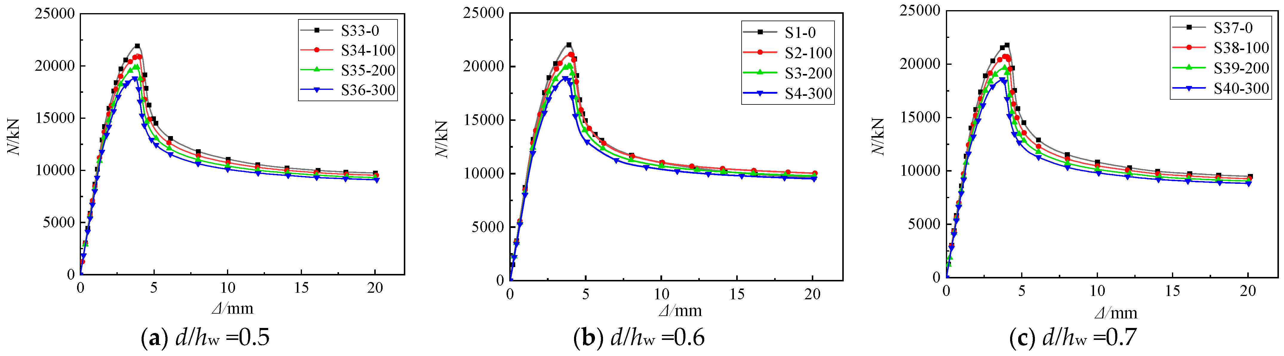
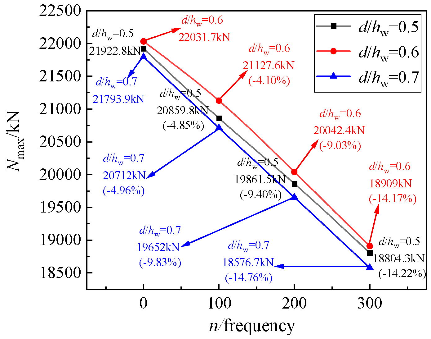
6.5. Aspect Ratio of Holes (d/hw)
7. Mechanism of Composite Columns under Axial Compression after Freeze–Thaw Cycles
7.1. Failure Modes of Specimens
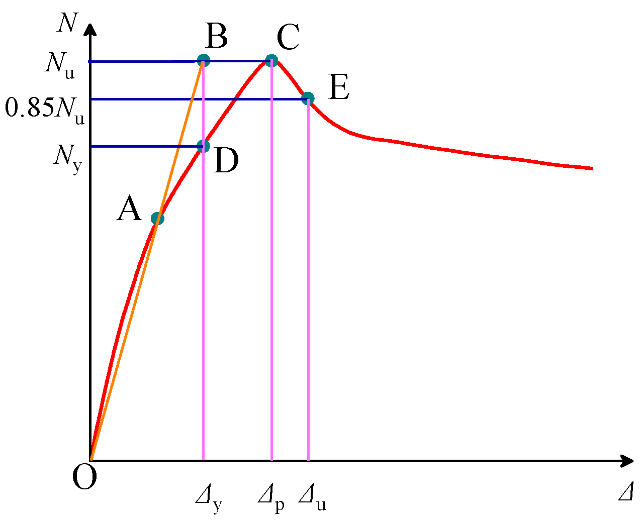
7.2. Analysis of the Load-Bearing Process of the Specimen
8. Equation for Ultimate Bearing Capacity of Composite Columns under Axial Compression after Freeze–Thaw Cycles
9. Conclusions
- (1)
- The load-bearing capacity of STHHC composite columns increases with an increase in ξ and fcu and decreases with a rise in λ. The influence of s/hw and d/hw on the ultimate load-bearing capacity of the composite columns is relatively small. The ductility of STHHC composite columns increases with the increase in ξ and decreases with a rise in λ and fcu. The impact of s/hw and d/hw on the ductility of the specimens is minimal.
- (2)
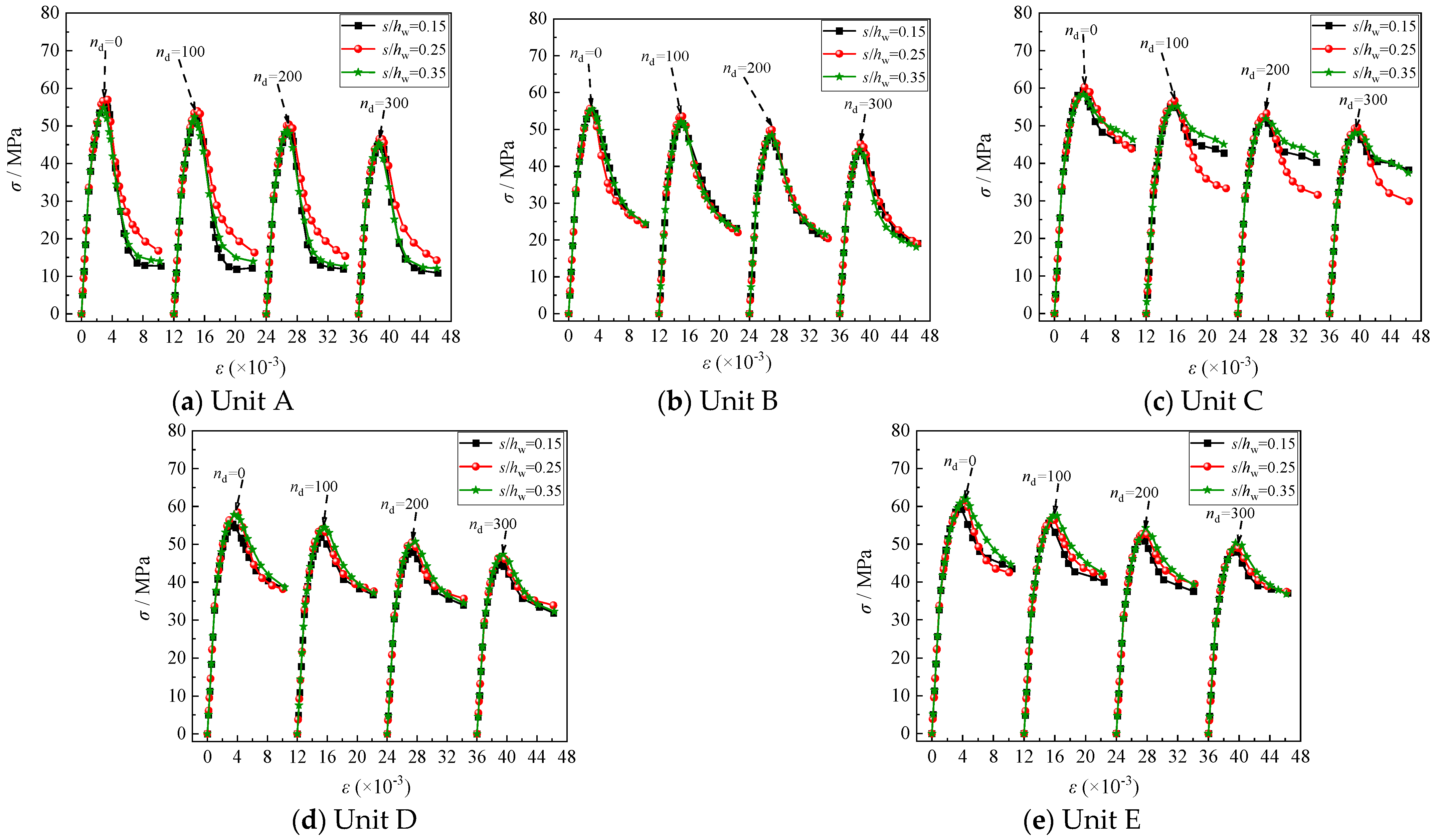
- As ξ increases, the rate of decrease in the ultimate load-carrying capacity of the specimens after freeze–thaw cycles (nd) gradually slows down. When ξ is between 0.23 and 0.48, the increase in ξ helps to mitigate the damage caused by the nd to the concrete, with more noticeable confinement effects in areas closer to the center of the specimen. As the concrete strength grade (fcu) increases, the degree of influence of nd lessens. The nd causes a certain degree of damage to the core concrete inside the steel tube. The higher the nd, the greater the degree of damage. As λ increases and the number of nd increases, the ultimate load-carrying capacity of the specimens will gradually decrease.
- (3)
- Moreover, the larger the λ, the greater the decrease in the ultimate load-carrying capacity of the specimens after nd, and the steel tube has a weaker confining effect on specimens, and the stress decrease in the central unit position is more apparent. With the increase in nd, the ductility of the composite column gradually decreases, but the numerical change is small, and the impact is minimal. Within the research range of this study, the larger the s/hw, the slower the rate of decrease in the ultimate load-carrying capacity. The change in d/hw has a minimal impact on the ultimate load-carrying capacity of the specimens after nd.
- (4)
- All specimens exhibited excellent load-bearing capacity and freeze–thaw resistance. During loading, the high-strength concrete and steel undergo synchronous deformation, causing the middle part of the specimen to bulge. At this time, the honeycomb steel web will gradually be compressed, and the honeycomb holes will become progressively elliptical. This indicates that the steel web also participates in the loading process. The web provides certain support to the concrete flanges on both sides of the steel tube, making the confining effect of the inner side of the flange more apparent.
- (5)
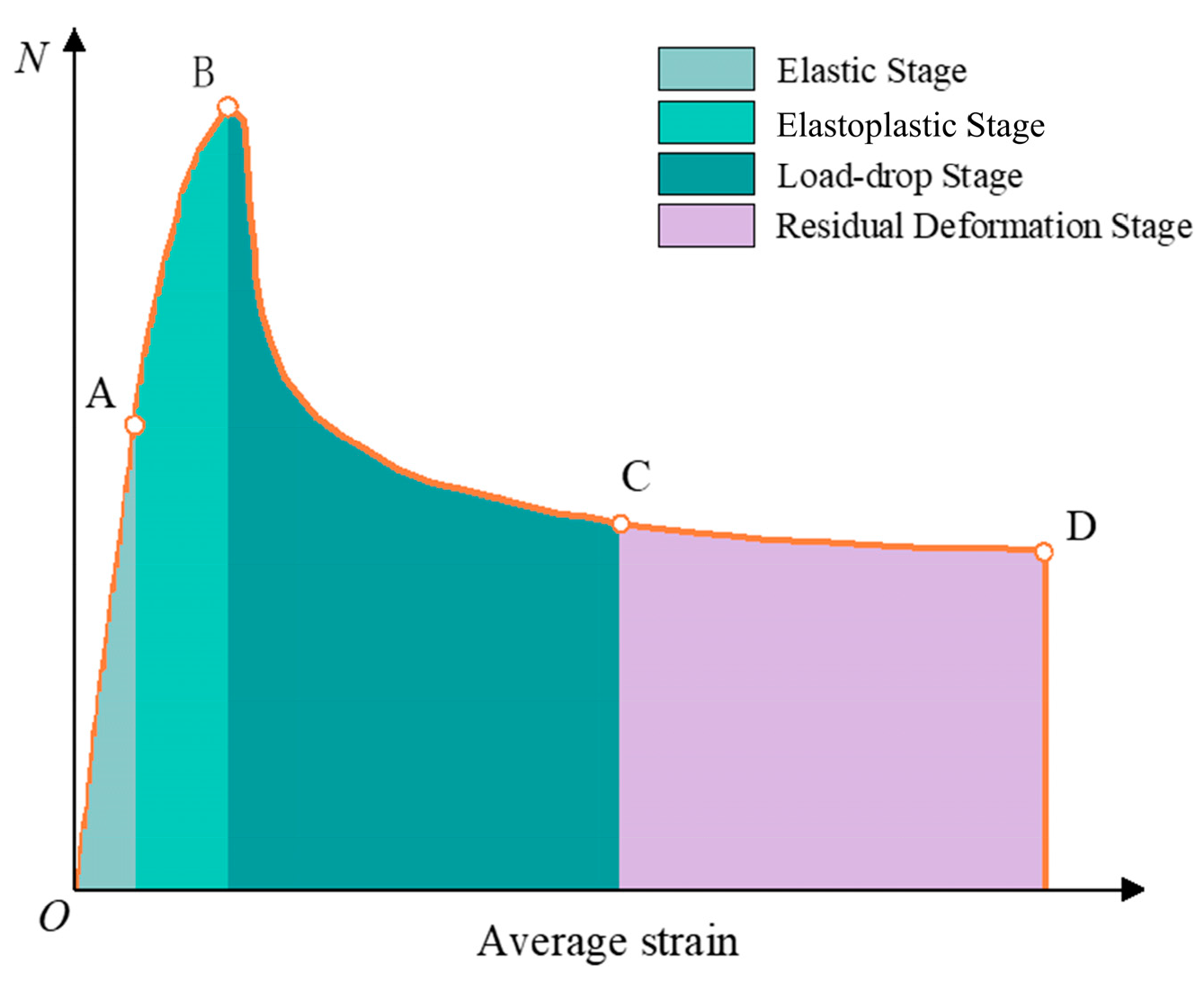
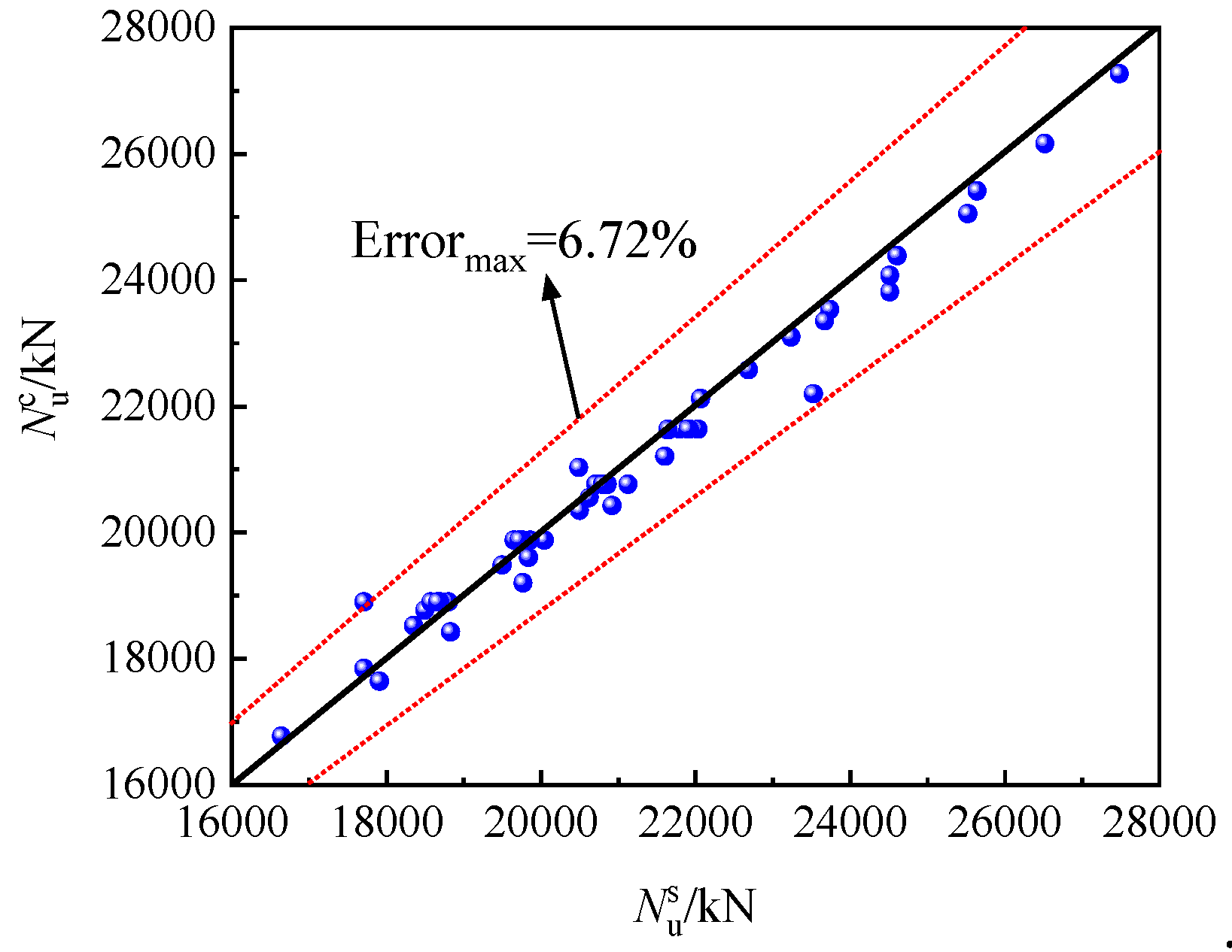
- STHHC composite columns that have undergone freeze–thaw cycles can be divided into four main stages when subjected to axial pressure: the elastic stage, the elastoplastic stage, the load decrease stage, and the residual deformation stage. Based on the consideration of the enhancement of the load-bearing capacity of the composite column by ξ and fcu, and the weakening of the load-bearing capacity by the web opening and nd, the 1stOpt software was used for fitting and regression to obtain the calculation equation for the axial load-bearing capacity of STHHC composite columns under freeze–thaw cycles. In comparing the ultimate load-bearing capacity calculated by the equation with that obtained from finite element analysis, the maximum error is 6.72%, which meets the engineering accuracy requirements.
- (6)
- In order to reduce the damage caused by the decrease in the bearing capacity caused by the freeze–thaw of concrete, it is suggested that the ξ of the composite column after freeze–thaw cycles should be controlled at about 0.48. From the perspectives of giving full play to material properties and the economy, it is recommended to use 70 MPa for fcu after freeze–thaw cycles. After a certain number of freeze–thaw cycles, the ultimate bearing capacity of the specimen will gradually decrease. At the same time, with the increase in the λ of the specimen, the decrease in the bearing capacity after the freeze–thaw cycles is greater. When the λ is between 11.08 and 11.78, the ultimate bearing capacity of the specimen decreases slightly under different freeze–thaw times. It is recommended that the λ is about 11.08. If the s/hw is too large, the initial stiffness of the composite column will be weakened. Therefore, it is recommended to use 0.6 for the s/hw of this type of composite column under freeze–thaw cycles. If the d/hw is too small, the initial stiffness of the composite column will be reduced, and if it is too large, the ductility of the specimen after freeze–thaw cycles will be reduced. Therefore, this paper suggests that the d/hw should be 0.25, and the thickness of the web should be 10 mm.
- (7)
- In this paper, the axial compression mechanical properties of STHHC composite columns under freeze–thaw cycles are analyzed. However, in practical engineering, members completely subjected to axial compression are rare. Therefore, in subsequent research, the eccentric compression mechanical properties of such composite columns after freeze–thaw cycles can be determined. The research on the axial compression performance in this paper is based on finite element simulation, and then the axial compression test of the STHHC composite columns under freeze–thaw cycles was carried out to compensate for the lack of experimental research in this paper. In addition, the concrete material used in this study was high-strength concrete. In the subsequent research, combined with the needs of modern buildings, new materials such as fiber-reinforced concrete, reactive powder concrete, and recycled concrete can be added to the steel pipe to study its mechanical properties under a freeze–thaw environment. The constitutive model provides technical support for the application of new materials.
Author Contributions
Funding
Data Availability Statement
Conflicts of Interest
References
- Sweedan, A.M.I.; El-Sawy, K.M. Elastic local buckling of perforated webs of steel cellular beam-column elements. J. Constr. Steel Res. 2011, 67, 1115–1127. [Google Scholar] [CrossRef]
- Sonck, D.; Belis, J. Weak-axis flexural buckling of cellular and castellated columns. J. Constr. Steel Res. 2016, 124, 91–100. [Google Scholar] [CrossRef]
- Ji, J.; Zhang, Z.; Lin, M.; Li, L.; Jiang, L.; Ding, Y.; Yu, K. Structural application of engineered cementitious composites (ECC): A state-of-the-art review. Constr. Build. Mater. 2023, 406, 133289. [Google Scholar] [CrossRef]
- Ucak, A.; Tsopelas, P. Cellular and corrugated cross-sectioned thin-walled steel bridge-piers/columns. Struct. Eng. Mech. 2006, 24, 355–374. [Google Scholar] [CrossRef]
- Lepcha, K.H.; Patton, M.L. A numerical study on structural behaviour of lean duplex stainless steel tubular beams with rectangular web openings. Structures 2021, 32, 1233–1249. [Google Scholar] [CrossRef]
- Ji, J.; Li, Y.H.; Jiang, L.Q. Axial compression behavior of strength-gradient composite stub columns encased CFST with small diameter: Experimental and numerical investigation. Structures 2023, 47, 282–298. [Google Scholar] [CrossRef]
- Ji, J.; Yang, M.M.; Xu, Z.C. Experimental Study of H-Shaped Honeycombed Stub Columns with Rectangular Concrete-Filled Steel Tube Flanges Subjected to Axial Load. Adv. Civ. Eng. 2021, 2021, 6678623. [Google Scholar] [CrossRef]
- Mohammed, H.S.; Ahmed, N.H.; Sherif, A.M. Numerical study on buckling of steel web plates with openings. Steel Compos. Struct. 2016, 22, 1417–1443. [Google Scholar]
- Ellobody, E. Nonlinear analysis of cellular steel beams under combined buckling modes. Thin Wall Struct. 2012, 52, 66–79. [Google Scholar] [CrossRef]
- Ji, J.; He, L.J.; Jiang, L.Q. Numerical study on the axial compression behavior of composite columns with steel tube SHCC flanges and honeycombed steel web. Eng. Struct. 2023, 283, 115883. [Google Scholar] [CrossRef]
- Chi, K.Y.; Li, J.; Wu, C.Q. Behaviour of reinforced concrete panels under impact loading after cryogenic freeze-thaw cycles. Constr. Build. Mater. 2024, 414, 135058. [Google Scholar] [CrossRef]
- Wang, H.; Wu, L.L.; Xu, X.; Lin, Z.B. Experimental study on bond durability of GFRP bar/engineered cementitious composite exposed to freeze-thaw environments. J. Build. 2024, 84, 108592. [Google Scholar] [CrossRef]
- Hong, L.; Li, M.M.; Du, C.M.; Huang, S.J.; Zhan, B.G.; Yu, Q.J. Bond behavior of the interface between concrete and basalt fiber reinforced polymer bar after freeze-thaw cycles. Front. Struct. Civ. Eng. 2024, 18, 630–641. [Google Scholar] [CrossRef]
- Abdelrahman, A.; Wael, A. Numerical parametric investigation on the moment redistribution of basalt FRC continuous beams with basalt FRP bars. Compos. Struct. 2021, 277, 114618. [Google Scholar]
- Sabih, M.S.; Hilo, J.S.; Hamood, J.M. Numerical Investigation into the Strengthening of Concrete-Filled Steel Tube Composite Columns Using Carbon Fiber-Reinforced Polymers. Buildings 2024, 14, 020441. [Google Scholar] [CrossRef]
- Xie, L.; Chen, M.C.; Huang, H. Experimental study on rectangular concrete-filled double-skin steel tubes subjected to eccentric compressive load. Ind. Constr. 2013, 43, 128–131. [Google Scholar]
- Ji, J.; Xu, Z.C.; Jiang, L.Q. Nonlinear buckling analysis of H-type honeycombed composite column with rectangular concrete-filled steel tube flanges. Build. Struct. 2018, 48, 50–55+70. [Google Scholar] [CrossRef]
- Ji, J. Experimental study on compression behavior of H-shaped composite short column with rectangular CFST flanges and honeycombed steel web subjected to axial load. J. Build. Struct. 2019, 40, 63–73. [Google Scholar]
- Elzeadani, M.; Bompa, D.V.; Elghazouli, A.Y. Axial compressive behaviour of composite steel elements incorporating rubberised alkali-activated concrete. J. Constr. Steel Res. 2023, 212, 108276. [Google Scholar] [CrossRef]
- Wei, W. Research on Eccentric Compressive Behavior of Round-Ended Concrete-Filled Steel Tubular Members. Master’s Thesis, Wuhan University of Technology, Wuhan, China, 2019. [Google Scholar]
- Ali, L.; Isleem, F.H.; Bahrami, A. Integrated behavioural analysis of FRP-confined circular columns using FEM and machine learning. Compos. Part C Open Access 2024, 13, 100444. [Google Scholar] [CrossRef]
- Shi, Y.L.; Zhang, C.F.; Xian, W.; Wang, W.D. Research on mechanical behavior of tapered concrete—Filled double skin steel tubular members under eccentric compression. J. Build. Struct. 2021, 42, 155–176. [Google Scholar]
- Ma, H.; Chen, Y.C.; Jia, M.L.; Cui, H.; Zhao, Y.L.; Li, Z. Nonlinear finite element analysis on mechanical behavior of SRRC filled square steel tube eccentric compression columns. Chinese J. Appl. Mech. 2021, 38, 2069–2078. [Google Scholar]
- Li, Y.H.; Zhang, S.M.; Wang, Y.; Wang, Y.Y. Deformation behavior of steel tube-cofined concrete-filled steel tube columns under systained axial compression. J. Harbin Inst. Technol. 2023, 55, 101–110. [Google Scholar]
- Chen, J.; Wang, Q.Z.; Guo, M.Q.; Zeng, L.H.; Zhang, X.B.; Tan, X.Y. Experimental study on the axial compression load capacity performance of short UHPC columns with high-strength steel pipes. J. Xiangtan Univ. (Nat. Sci. Ed.) 2024, 46, 20–34. [Google Scholar]
- Ji, J.; Xu, Z.C.; Jiang, L.Q.; Zhang, Y.F.; Zhou, L.J.; Zhang, S.L. Nonlinear buckling analysis of H-type honeycombed composite column with rectangular concrete-filled steel tube flanges. Int. J. Steel Struct. 2018, 18, 1153–1166. [Google Scholar] [CrossRef]
- Gao, S.; Zhang, K.Y.; Li, J.Q.; Xu, Y.C.; Wang, Y.G. Experimental study on axial performance of circular CFST under freeze-thaw and corrosion complex environment. J. Nat. Disasters 2021, 30, 93–100. [Google Scholar]
- Li, X.E.; Miao, J.J.; Zeng, Z.P.; Chen, C. Study on bearing capacity of circular CFST stub column after being exposed to freeze- thaw cycles. J. Civil. Environ. Eng. 2023, 45, 114–123. [Google Scholar]
- Zhou, L.Q.; Gao, S.; Zhang, K.Y.; Chang, C.; Peng, Z. Experimental study on axial performance of circular CFST under freeze-thaw and corrosion complex environment. Concrete 2022, 08, 15–19+24. [Google Scholar]
- Gao, S.L.; Liu, L.Y. Effects of Freeze-Thaw Cycles on Axial Compression Behaviors of UHPC-RC Composite Columns. Materials 2024, 17, 17081843. [Google Scholar] [CrossRef]
- Pagoulatou, M.; Sheehan, T.; Dai, X.H. Finite element analysis on the capacity of circular concrete-filled double-skin steel tubular (CFDST) stub columns. Eng. Struct. 2014, 72, 102–112. [Google Scholar] [CrossRef]
- Su, Y.M. Analysis on Axial Compressive Behavior of Reinforced Concrete Short Columns after Freeze-Thaw Cycles. Master’s Thesis, Dalian University of Technology, Dalian, China, 2021. [Google Scholar]
- Cao, K. Study on Performance of Concrete Filled Steel Tubular Stub Columns after Being to Exposed Freezing and Thawing. Master’s Thesis, Dalian University of Technology, Dalian, China, 2013. [Google Scholar]
- Ji, J.; Yu, C.Y.; Jiang, L.Q. Bearing Behavior of H-Shaped Honeycombed Steel Web Composite Columns with Rectangular Concrete-Filled Steel Tube Flanges under Eccentrical Compression Load. Adv. Civ. Eng. 2022, 2022, 2965131. [Google Scholar] [CrossRef]
- Ji, J.; Jiang, L.; Jiang, L.Q. Eccentric compression performance of H-type cellular composite medium-long columns with rectangular concrete-filled steel tubular flanges. J. Northeast Petroleum Univ. 2020, 44, 121–132. [Google Scholar]
- Han, L.H.; Tao, Z. Theoretical analysis and experimental study on axial compressive mechanical properties of concrete-filled square steel tube. China Civil. Eng. J. 2001, 2, 17–25. [Google Scholar]
- Ji, J.; Lin, Y.B.; Jiang, L.Q. Hysteretic behavior of H-shaped honeycombed steel web composite columns with rectangular concrete-filled steel tube flanges. Adv. Civ. Eng. 2022, 2022, 1546263. [Google Scholar] [CrossRef]
- Yang, Y.F.; Cao, K.; Yang, Z.Q.; Lin, J. Mechanical properties of concrete filled steel tubular stubs after freezing and thawing cycles under axial loading. China J. Hwy. Transp. 2014, 27, 51–58. [Google Scholar]


| Specimens | b × h1 × hw × t2 × t1/mm | L/mm | λ | nd | ξ | fyk/MPa | fcu/MPa | d/hw | s/hw |
|---|---|---|---|---|---|---|---|---|---|
| STHHC-1 | 500 × 320 × 400 × 10 × 04 | 1600 | 11.08 | 0 | 0.23 | 345 | 70 | 0.6 | 0.25 |
| STHHC-2 | 500 × 320 × 400 × 10 × 04 | 1600 | 11.08 | 100 | 0.23 | 345 | 70 | 0.6 | 0.25 |
| STHHC-3 | 500 × 320 × 400 × 10 × 04 | 1600 | 11.08 | 200 | 0.23 | 345 | 70 | 0.6 | 0.25 |
| STHHC-4 | 500 × 320 × 400 × 10 × 04 | 1600 | 11.08 | 300 | 0.23 | 345 | 70 | 0.6 | 0.25 |
| STHHC-5 | 500 × 320 × 400 × 10 × 06 | 1600 | 11.08 | 0 | 0.35 | 345 | 70 | 0.6 | 0.25 |
| STHHC-6 | 500 × 320 × 400 × 10 × 06 | 1600 | 11.08 | 100 | 0.35 | 345 | 70 | 0.6 | 0.25 |
| STHHC-7 | 500 × 320 × 400 × 10 × 06 | 1600 | 11.08 | 200 | 0.35 | 345 | 70 | 0.6 | 0.25 |
| STHHC-8 | 500 × 320 × 400 × 10 × 06 | 1600 | 11.08 | 300 | 0.35 | 345 | 70 | 0.6 | 0.25 |
| STHHC-9 | 500 × 320 × 400 × 10 × 08 | 1600 | 11.08 | 0 | 0.48 | 345 | 70 | 0.6 | 0.25 |
| STHHC-10 | 500 × 320 × 400 × 10 × 08 | 1600 | 11.08 | 100 | 0.48 | 345 | 70 | 0.6 | 0.25 |
| STHHC-11 | 500 × 320 × 400 × 10 × 08 | 1600 | 11.08 | 200 | 0.48 | 345 | 70 | 0.6 | 0.25 |
| STHHC-12 | 500 × 320 × 400 × 10 × 08 | 1600 | 11.08 | 300 | 0.48 | 345 | 70 | 0.6 | 0.25 |
| STHHC-13 | 500 × 320 × 400 × 10 × 10 | 1600 | 11.08 | 0 | 0.60 | 345 | 70 | 0.6 | 0.25 |
| STHHC-14 | 500 × 320 × 400 × 10 × 10 | 1600 | 11.08 | 100 | 0.60 | 345 | 70 | 0.6 | 0.25 |
| STHHC-15 | 500 × 320 × 400 × 10 × 10 | 1600 | 11.08 | 200 | 0.60 | 345 | 70 | 0.6 | 0.25 |
| STHHC-16 | 500 × 320 × 400 × 10 × 10 | 1600 | 11.08 | 300 | 0.60 | 345 | 70 | 0.6 | 0.25 |
| STHHC-17 | 500 × 320 × 400 × 10 × 04 | 1600 | 11.08 | 0 | 0.27 | 345 | 60 | 0.6 | 0.25 |
| STHHC-18 | 500 × 320 × 400 × 10 × 04 | 1600 | 11.08 | 100 | 0.27 | 345 | 60 | 0.6 | 0.25 |
| STHHC-19 | 500 × 320 × 400 × 10 × 04 | 1600 | 11.08 | 200 | 0.27 | 345 | 60 | 0.6 | 0.25 |
| STHHC-20 | 500 × 320 × 400 × 10 × 04 | 1600 | 11.08 | 300 | 0.27 | 345 | 60 | 0.6 | 0.25 |
| STHHC-21 | 500 × 320 × 400 × 10 × 04 | 1600 | 11.08 | 0 | 0.20 | 345 | 80 | 0.6 | 0.25 |
| STHHC-22 | 500 × 320 × 400 × 10 × 04 | 1600 | 11.08 | 100 | 0.20 | 345 | 80 | 0.6 | 0.25 |
| STHHC-23 | 500 × 320 × 400 × 10 × 04 | 1600 | 11.08 | 200 | 0.20 | 345 | 80 | 0.6 | 0.25 |
| STHHC-24 | 500 × 320 × 400 × 10 × 04 | 1600 | 11.08 | 300 | 0.20 | 345 | 80 | 0.6 | 0.25 |
| STHHC-25 | 500 × 320 × 400 × 10 × 04 | 1700 | 11.78 | 0 | 0.23 | 345 | 70 | 0.6 | 0.25 |
| STHHC-26 | 500 × 320 × 400 × 10 × 04 | 1700 | 11.78 | 100 | 0.23 | 345 | 70 | 0.6 | 0.25 |
| STHHC-27 | 500 × 320 × 400 × 10 × 04 | 1700 | 11.78 | 200 | 0.23 | 345 | 70 | 0.6 | 0.25 |
| STHHC-28 | 500 × 320 × 400 × 10 × 04 | 1700 | 11.78 | 300 | 0.23 | 345 | 70 | 0.6 | 0.25 |
| STHHC-29 | 500 × 320 × 400 × 10 × 04 | 1800 | 12.47 | 0 | 0.23 | 345 | 70 | 0.6 | 0.25 |
| STHHC-30 | 500 × 320 × 400 × 10 × 04 | 1800 | 12.47 | 100 | 0.23 | 345 | 70 | 0.6 | 0.25 |
| STHHC-31 | 500 × 320 × 400 × 10 × 04 | 1800 | 12.47 | 200 | 0.23 | 345 | 70 | 0.6 | 0.25 |
| STHHC-32 | 500 × 320 × 400 × 10 × 04 | 1800 | 12.47 | 300 | 0.23 | 345 | 70 | 0.6 | 0.25 |
| STHHC-33 | 500 × 320 × 400 × 10 × 04 | 1600 | 11.08 | 0 | 0.23 | 345 | 70 | 0.5 | 0.25 |
| STHHC-34 | 500 × 320 × 400 × 10 × 04 | 1600 | 11.08 | 100 | 0.23 | 345 | 70 | 0.5 | 0.25 |
| STHHC-35 | 500 × 320 × 400 × 10 × 04 | 1600 | 11.08 | 200 | 0.23 | 345 | 70 | 0.5 | 0.25 |
| STHHC-36 | 500 × 320 × 400 × 10 × 04 | 1600 | 11.08 | 300 | 0.23 | 345 | 70 | 0.5 | 0.25 |
| STHHC-37 | 500 × 320 × 400 × 10 × 04 | 1600 | 11.08 | 0 | 0.23 | 345 | 70 | 0.7 | 0.25 |
| STHHC-38 | 500 × 320 × 400 × 10 × 04 | 1600 | 11.08 | 100 | 0.23 | 345 | 70 | 0.7 | 0.25 |
| STHHC-39 | 500 × 320 × 400 × 10 × 04 | 1600 | 11.08 | 200 | 0.23 | 345 | 70 | 0.7 | 0.25 |
| STHHC-40 | 500 × 320 × 400 × 10 × 04 | 1600 | 11.08 | 300 | 0.23 | 345 | 70 | 0.7 | 0.25 |
| STHHC-41 | 500 × 320 × 400 × 10 × 04 | 1600 | 11.08 | 0 | 0.23 | 345 | 70 | 0.6 | 0.15 |
| STHHC-42 | 500 × 320 × 400 × 10 × 04 | 1600 | 11.08 | 100 | 0.23 | 345 | 70 | 0.6 | 0.15 |
| STHHC-43 | 500 × 320 × 400 × 10 × 04 | 1600 | 11.08 | 200 | 0.23 | 345 | 70 | 0.6 | 0.15 |
| STHHC-44 | 500 × 320 × 400 × 10 × 04 | 1600 | 11.08 | 300 | 0.23 | 345 | 70 | 0.6 | 0.15 |
| STHHC-45 | 500 × 320 × 400 × 10 × 04 | 1600 | 11.08 | 0 | 0.23 | 345 | 70 | 0.6 | 0.35 |
| STHHC-46 | 500 × 320 × 400 × 10 × 04 | 1600 | 11.08 | 100 | 0.23 | 345 | 70 | 0.6 | 0.35 |
| STHHC-47 | 500 × 320 × 400 × 10 × 04 | 1600 | 11.08 | 200 | 0.23 | 345 | 70 | 0.6 | 0.35 |
| STHHC-48 | 500 × 320 × 400 × 10 × 04 | 1600 | 11.08 | 300 | 0.23 | 345 | 70 | 0.6 | 0.35 |
| Specimens | h1 × b × hw × t2 × t1/mm | λ | l/mm | ξ | fyk/MPa | fcu/MPa | /kN | /kN | |
|---|---|---|---|---|---|---|---|---|---|
| STHHC-1 | 50 × 100 × 100 × 6 × 1.7 | 12.82 | 370 | 0.60 | 269 | 49.50 | 740.0 | 763.4 | 3.17% |
| STHHC-2 | 50 × 100 × 100 × 6 × 2.3 | 12.82 | 370 | 0.88 | 282 | 49.50 | 871.7 | 864.5 | 0.83% |
| STHHC-3 | 50 × 100 × 100 × 6 × 3.8 | 12.82 | 370 | 1.60 | 286 | 49.50 | 1175.6 | 1150.8 | 2.11% |
| STHHC-4 | 50 × 100 × 100 × 6 × 2.3 | 12.82 | 370 | 0.82 | 282 | 53.17 | 1070.4 | 1057.4 | 1.21% |
| STHHC-5 | 50 × 100 × 100 × 6 × 2.3 | 12.82 | 370 | 0.66 | 282 | 55.69 | 1172.7 | 1152.3 | 1.73% |
| STHHC-6 | 50 × 100 × 100 × 6 × 2.3 | 12.82 | 370 | 0.78 | 282 | 65.60 | 1015.9 | 1020.1 | 0.41% |
| STHHC-7 | 50 × 100 × 100 × 8 × 1.7 | 12.82 | 370 | 0.60 | 269 | 49.50 | 752.6 | 789.6 | 4.91% |
| STHHC-8 | 50 × 100 × 100 × 11 × 2.7 | 12.82 | 370 | 0.60 | 269 | 49.50 | 796.7 | 834.1 | 4.69% |
| STHHC-9 | 50 × 100 × 100 × 6 × 2.3 | 9.35 | 270 | 0.88 | 282 | 49.50 | 947.0 | 936.9 | 1.06% |
| STHHC-10 | 50 × 100 × 100 × 6 × 2.3 | 16.28 | 470 | 0.88 | 282 | 49.50 | 841.1 | 829.0 | 1.36% |
| STHHC-11 | 50 × 100 × 100 × 6 × 1.7 | 9.35 | 270 | 0.60 | 269 | 49.50 | 772.9 | 787.8 | 1.93% |
| STHHC-12 | 50 × 100 × 100 × 6 × 1.7 | 16.28 | 470 | 0.60 | 269 | 49.50 | 741.1 | 762.8 | 2.92% |
| STHHC-13 | 50 × 100 × 100 × 6 × 3.8 | 9.35 | 270 | 1.60 | 286 | 49.50 | 1276.0 | 1299.1 | 1.81% |
| STHHC-14 | 50 × 100 × 100 × 6 × 3.8 | 16.28 | 470 | 1.60 | 286 | 49.50 | 1069.0 | 1080.5 | 1.07% |
| Specimens | D/mm | L/mm | t/mm | fcu/MPa | α | fy/MPa | /kN | /kN | |
|---|---|---|---|---|---|---|---|---|---|
| SC2-0 | 100 | 300 | 2.06 | 63.7 | 0.113 | 338.4 | 808.38 | 834.96 | 3.34% |
| SC2-50 | 100 | 300 | 2.06 | 63.7 | 0.113 | 338.4 | 803.00 | 785.81 | 2.13% |
| SC2-100 | 100 | 300 | 2.06 | 63.7 | 0.113 | 338.4 | 783.77 | 802.04 | 2.32% |
| SC2-200 | 100 | 300 | 2.06 | 63.7 | 0.113 | 338.4 | 808.99 | 832.09 | 2.83% |
| SC2-300 | 100 | 300 | 2.06 | 63.7 | 0.113 | 338.4 | 749.10 | 775.16 | 3.41% |
| S2-0 | 100 | 300 | 2.00 | 83.9 | 0.085 | 184.7 | 861.67 | 814.23 | 5.83% |
| S2-50 | 100 | 300 | 2.00 | 83.9 | 0.085 | 184.7 | 804.47 | 793.24 | 1.42% |
| S2-100 | 100 | 300 | 2.00 | 83.9 | 0.085 | 184.7 | 783.92 | 778.60 | 0.68% |
| S2-200 | 100 | 300 | 2.00 | 83.9 | 0.085 | 184.7 | 777.55 | 754.89 | 3.00% |
| S2-300 | 100 | 300 | 2.00 | 83.9 | 0.085 | 184.7 | 663.06 | 715.48 | 7.91% |
| S3-0 | 100 | 300 | 3.00 | 83.9 | 0.132 | 176.5 | 891.58 | 856.82 | 4.06% |
| S3-50 | 100 | 300 | 3.00 | 83.9 | 0.132 | 176.5 | 873.91 | 852.65 | 2.49% |
| S3-100 | 100 | 300 | 3.00 | 83.9 | 0.132 | 176.5 | 775.53 | 800.38 | 3.20% |
| S3-200 | 100 | 300 | 3.00 | 83.9 | 0.132 | 176.5 | 754.48 | 815.90 | 8.14% |
| S3-300 | 100 | 300 | 3.00 | 83.9 | 0.132 | 176.5 | 722.31 | 772.20 | 6.91% |
| Specimens | nd | fcu/MPa | λ | fyk /MPa | ξ | /kN | /kN | |
|---|---|---|---|---|---|---|---|---|
| S1 | 0 | 70 | 11.08 | 345 | 0.23 | 22,031.7 | 21,639.1 | 1.78% |
| S2 | 100 | 70 | 11.08 | 345 | 0.23 | 21,127.6 | 20,764.7 | 1.72% |
| S3 | 200 | 70 | 11.08 | 345 | 0.23 | 20,042.4 | 19,882.9 | 0.80% |
| S4 | 300 | 70 | 11.08 | 345 | 0.23 | 17,710.2 | 18,900.1 | 6.72% |
| S5 | 0 | 70 | 11.08 | 345 | 0.35 | 23,737.4 | 23,534.9 | 0.85% |
| S6 | 100 | 70 | 11.08 | 345 | 0.35 | 22,685.6 | 22,583.9 | 0.45% |
| S7 | 200 | 70 | 11.08 | 345 | 0.35 | 21,646.8 | 21,624.8 | 0.10% |
| S8 | 300 | 70 | 11.08 | 345 | 0.35 | 20,624.8 | 20,555.9 | 0.33% |
| S9 | 0 | 70 | 11.08 | 345 | 0.48 | 25,641.7 | 25,414.8 | 0.88% |
| S10 | 100 | 70 | 11.08 | 345 | 0.48 | 24,605.8 | 24,387.9 | 0.89% |
| S11 | 200 | 70 | 11.08 | 345 | 0.48 | 23,670.1 | 23,352.2 | 1.34% |
| S12 | 300 | 70 | 11.08 | 345 | 0.48 | 23,524.9 | 22,197.9 | 5.64% |
| S13 | 0 | 70 | 11.08 | 345 | 0.6 | 27,481.6 | 27,268.7 | 0.77% |
| S14 | 100 | 70 | 11.08 | 345 | 0.6 | 26,518.8 | 26,166.8 | 1.33% |
| S15 | 200 | 70 | 11.08 | 345 | 0.6 | 25,520.2 | 25,055.6 | 1.82% |
| S16 | 300 | 70 | 11.08 | 345 | 0.6 | 24,511.1 | 23,817.1 | 2.83% |
| S17 | 0 | 60 | 11.08 | 345 | 0.27 | 19,766.7 | 19,201.6 | 2.86% |
| S18 | 100 | 60 | 11.08 | 345 | 0.27 | 18,832.9 | 18,425.7 | 2.16% |
| S19 | 200 | 60 | 11.08 | 345 | 0.27 | 17,912.1 | 17,643.3 | 1.50% |
| S20 | 300 | 60 | 11.08 | 345 | 0.27 | 16,642.0 | 16,771.1 | 0.78% |
| S21 | 0 | 80 | 11.08 | 345 | 0.2 | 24,511.7 | 24,076.6 | 1.78% |
| S22 | 100 | 80 | 11.08 | 345 | 0.2 | 23,233.5 | 23,103.7 | 0.56% |
| S23 | 200 | 80 | 11.08 | 345 | 0.2 | 22,065.3 | 22,122.6 | 0.26% |
| S24 | 300 | 80 | 11.08 | 345 | 0.2 | 20,489.6 | 21,029.0 | 2.63% |
| S25 | 0 | 70 | 11.78 | 345 | 0.23 | 21,603.4 | 21,206.8 | 1.84% |
| S26 | 100 | 70 | 11.78 | 345 | 0.23 | 20,500.0 | 20,349.9 | 0.73% |
| S27 | 200 | 70 | 11.78 | 345 | 0.23 | 19,500.0 | 19,485.7 | 0.07% |
| S28 | 300 | 70 | 11.78 | 345 | 0.23 | 18,355.2 | 18,522.5 | 0.91% |
| S29 | 0 | 70 | 12.47 | 345 | 0.23 | 20,920.9 | 20,428.8 | 2.35% |
| S30 | 100 | 70 | 12.47 | 345 | 0.23 | 19,839.5 | 19,603.3 | 1.19% |
| S31 | 200 | 70 | 12.47 | 345 | 0.23 | 18,500.0 | 18,770.9 | 1.46% |
| S32 | 300 | 70 | 12.47 | 345 | 0.23 | 17,710.2 | 17,843.0 | 0.75% |
Disclaimer/Publisher’s Note: The statements, opinions and data contained in all publications are solely those of the individual author(s) and contributor(s) and not of MDPI and/or the editor(s). MDPI and/or the editor(s) disclaim responsibility for any injury to people or property resulting from any ideas, methods, instructions or products referred to in the content. |
© 2024 by the authors. Licensee MDPI, Basel, Switzerland. This article is an open access article distributed under the terms and conditions of the Creative Commons Attribution (CC BY) license (https://creativecommons.org/licenses/by/4.0/).
Share and Cite
Ji, J.; Xu, Y.; Jiang, L.; Yuan, C.; Liu, Y.; Hou, X.; Li, J.; Zhang, Z.; Chu, X.; Ma, G. Numerical Study on the Axial Compression Behavior of Composite Columns with High-Strength Concrete-Filled Steel Tube and Honeycombed Steel Web Subjected to Freeze–Thaw Cycles. Buildings 2024, 14, 2401. https://doi.org/10.3390/buildings14082401
Ji J, Xu Y, Jiang L, Yuan C, Liu Y, Hou X, Li J, Zhang Z, Chu X, Ma G. Numerical Study on the Axial Compression Behavior of Composite Columns with High-Strength Concrete-Filled Steel Tube and Honeycombed Steel Web Subjected to Freeze–Thaw Cycles. Buildings. 2024; 14(8):2401. https://doi.org/10.3390/buildings14082401
Chicago/Turabian StyleJi, Jing, Yihuan Xu, Liangqin Jiang, Chaoqing Yuan, Yingchun Liu, Xiaomeng Hou, Jinbao Li, Zhanbin Zhang, Xuan Chu, and Guiling Ma. 2024. "Numerical Study on the Axial Compression Behavior of Composite Columns with High-Strength Concrete-Filled Steel Tube and Honeycombed Steel Web Subjected to Freeze–Thaw Cycles" Buildings 14, no. 8: 2401. https://doi.org/10.3390/buildings14082401