
Data-Driven Prediction of Electrical Resistivity of Graphene Oxide/Cement Composites Considering the Effects of Specimen Size and Measurement Method

 ,
,  , , , and
Abstract
1. Introduction
2. Data Collection and Pre-Processing
3. Methodology
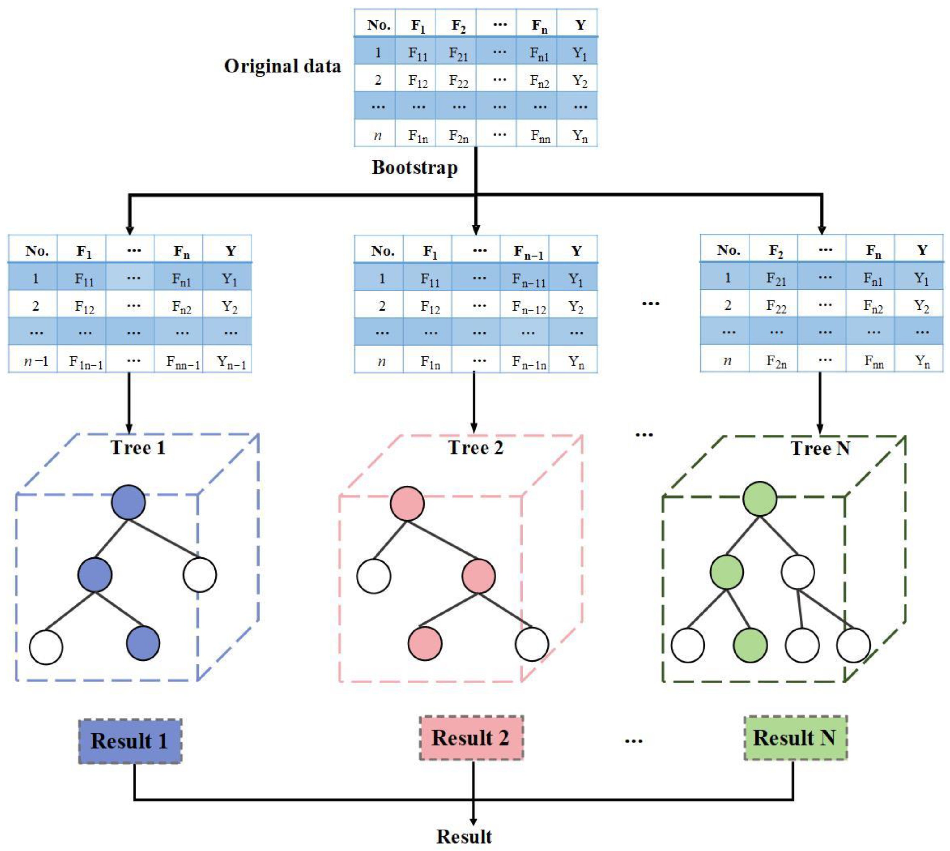
3.1. Random Forest
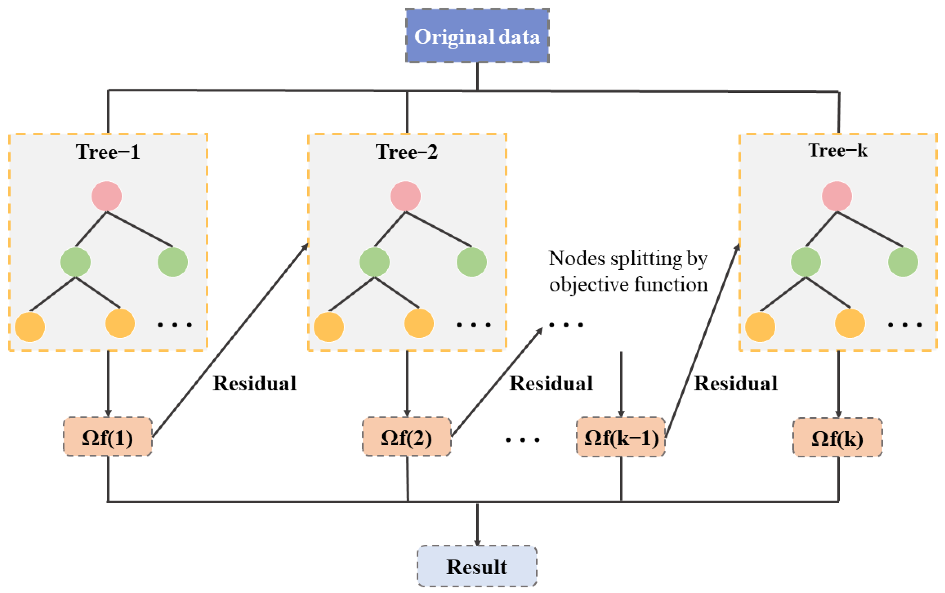
3.2. Extreme Gradient Boosting
3.3. Artificial Neural Network
3.4. Evaluation Metrics
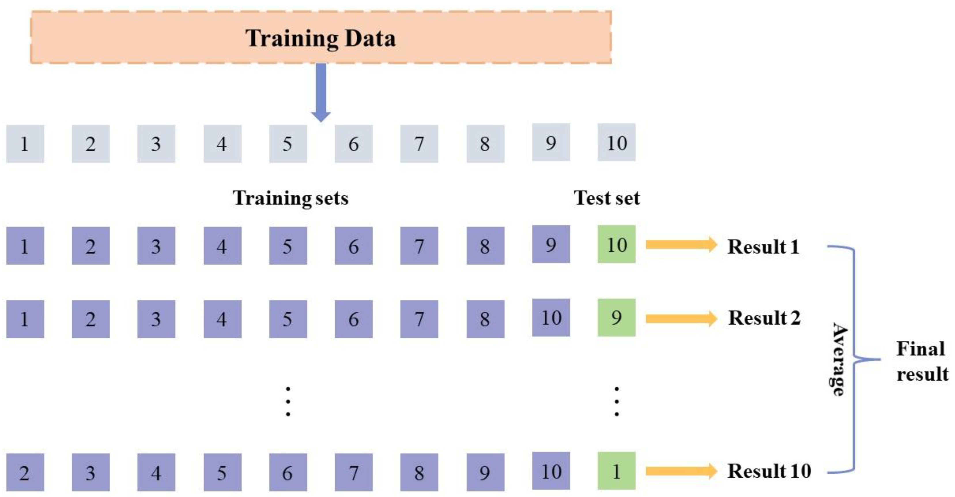
3.5. K-Fold Cross-Validation
- (1)
- Divide the original dataset into k folds of mutually exclusive subsets with equal size.
- (2)
- For each round, one fold is selected as the test set and the remaining folds are used as the training set. The model is trained, and its performance is evaluated by the test set. Repeat this process until each fold has been used as a test set.
- (3)
- The results of each round of the model evaluation are summarized, and the final output is the average of the results of the k rounds.
4. Results and Discussion
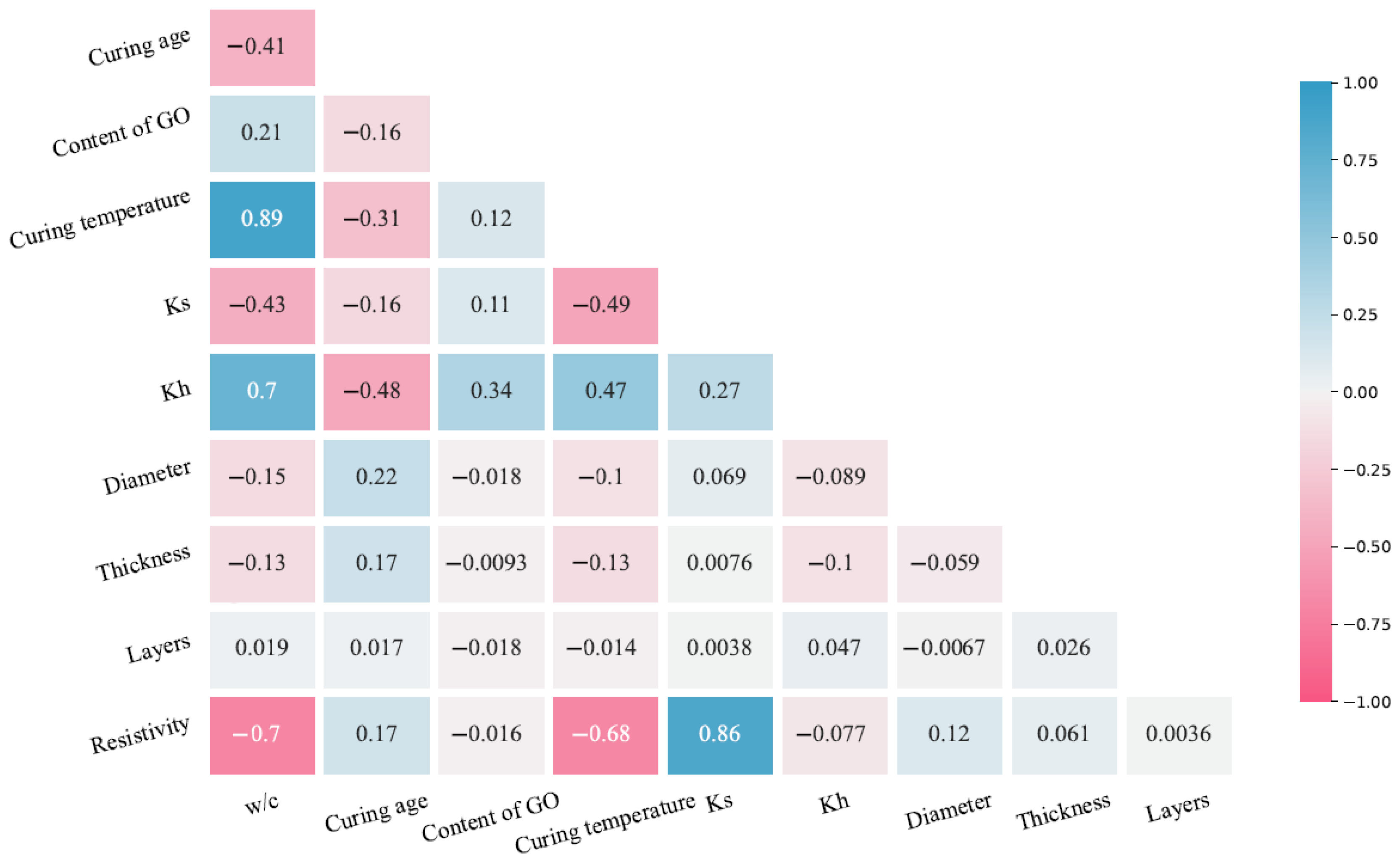
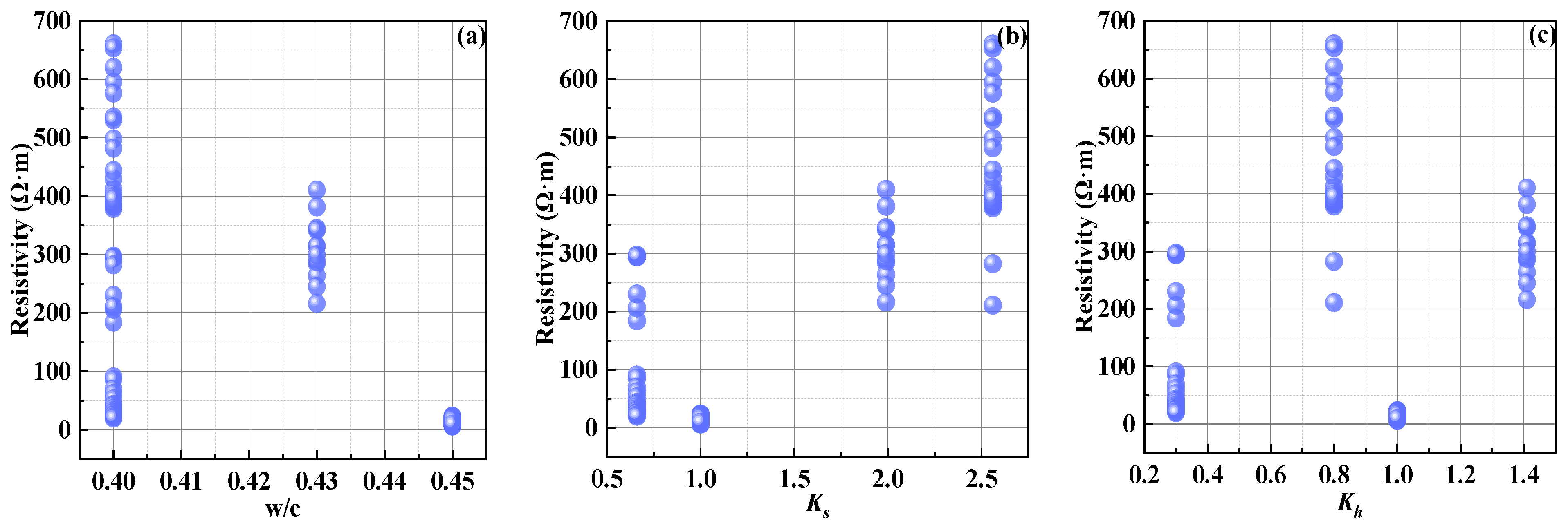
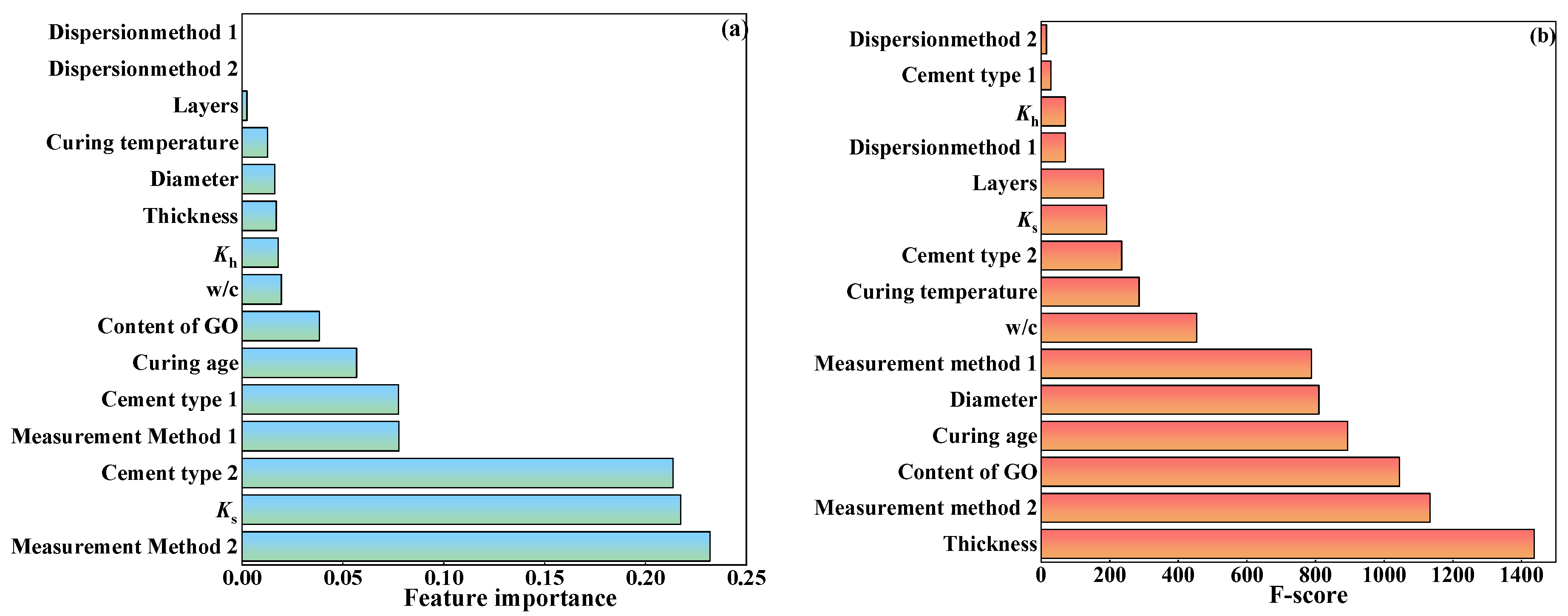
4.1. Correlation Analysis
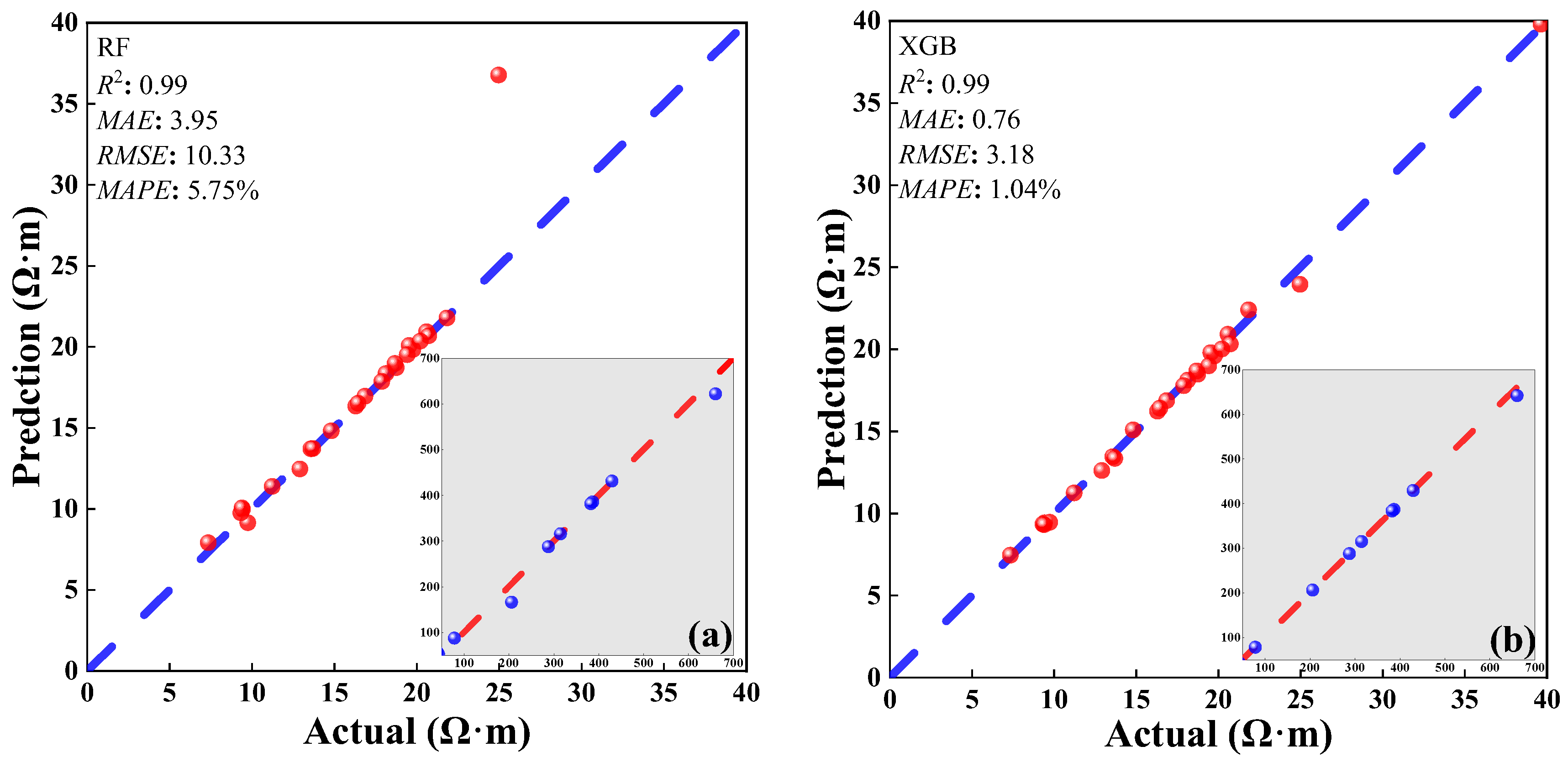
4.2. Electrical Resistivity by RF and XGB
4.3. Electrical Resistivity by ANN
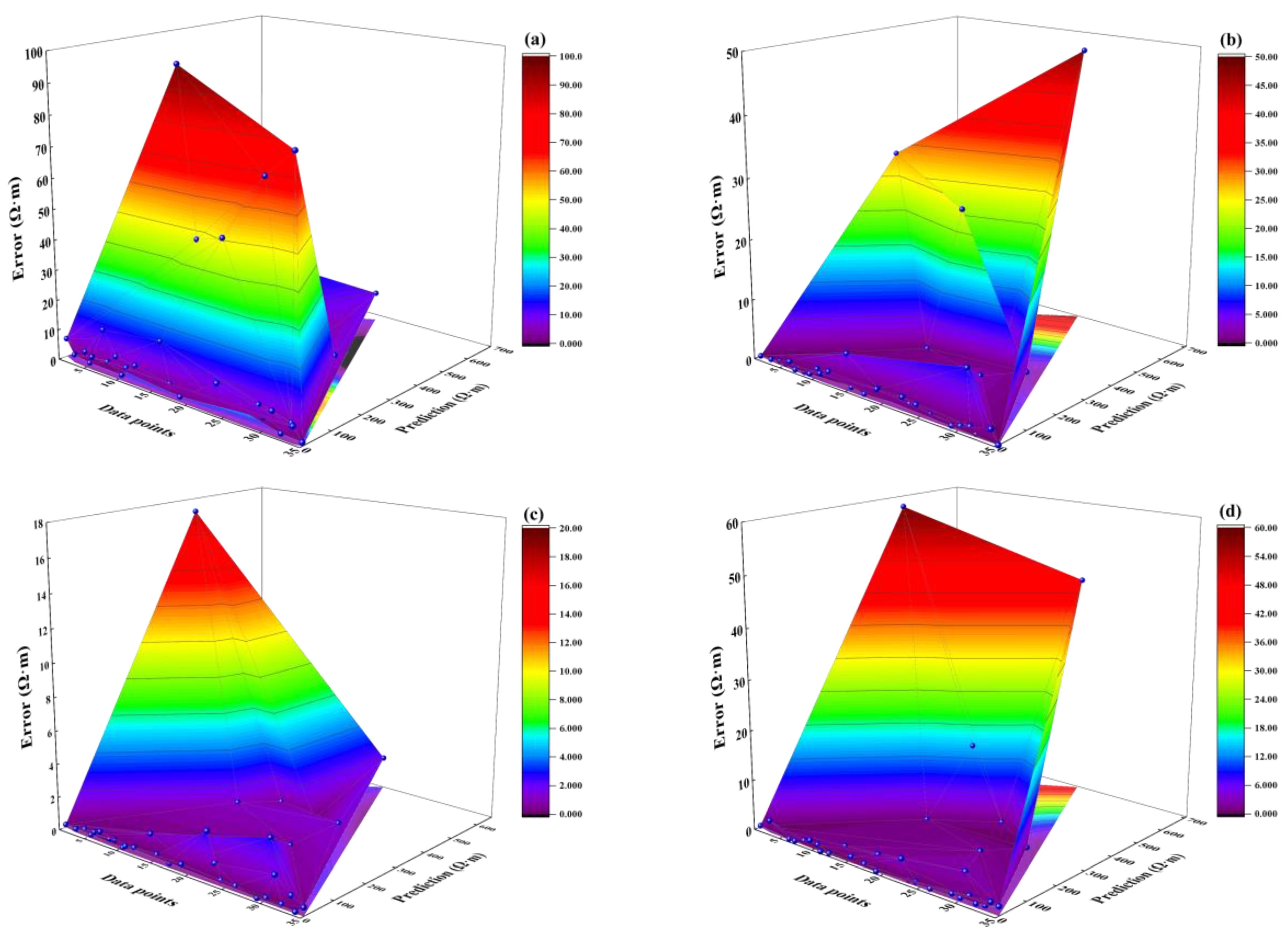
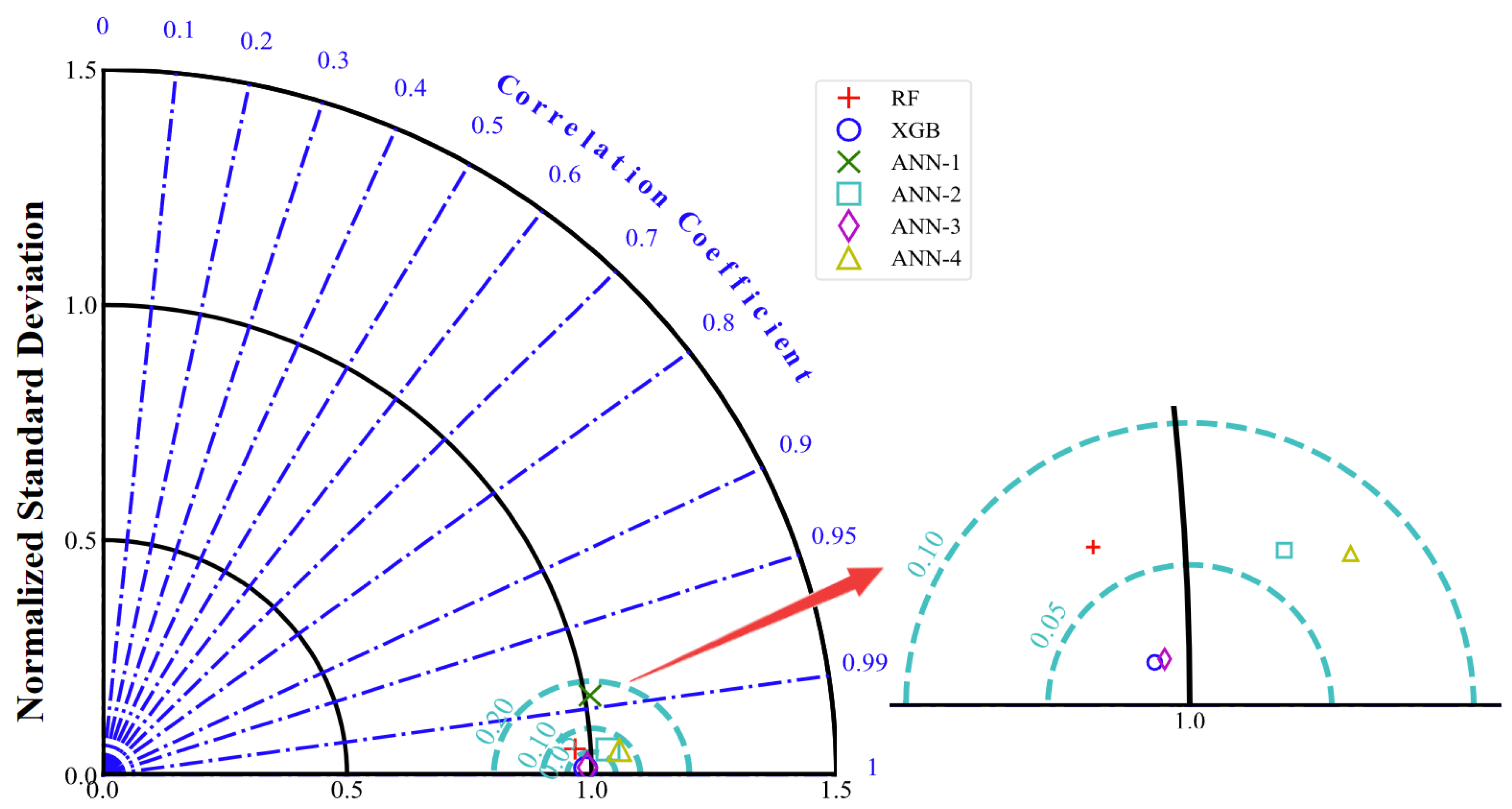
4.4. Comparison of Performance Evaluation for Different Models
5. Conclusions
- (1)
- The three ML models are evidenced to be capable of predicting the resistivity of the GORCCs, which suggests that ML is promising for practical applications in the field of identifying the nonlinear and complex relationship between the material properties and various influencing factors.
- (2)
- The structure of the ANN has a significant impact on the prediction performance. It is found that the ANN model with hidden layers may increase the learning ability of the network, allowing it to better fit complex data patterns. However, more hidden layers may lead to overfitting and are not always favorable for improving the prediction performance. The ANN model with the structure of 15-64-32-16-1 is proven to have the best performance in this work. This can provide useful guidelines when conducting ML modeling for predicting the material properties.
- (3)
- The strong correlation between specimen size and the resistivity suggests that the consideration of the specimen size is important for accurate capture of the material properties. In addition, it is found that the electrical resistivity of the GORCCs is also highly dependent on the measurement method. This observation is of great importance when selecting the measurement method to obtain accurate and objective experimental data.
Author Contributions
Funding
Data Availability Statement
Conflicts of Interest
Appendix A

| No. | Type of Cement | Dispersion Method | Measurement Method | w/c | Curing Temperature | Curing Age | Ks | Kh | Diameter (μm) | Thickness (nm) | Layers | GO Content | Electrical Resistivity | Reference |
|---|---|---|---|---|---|---|---|---|---|---|---|---|---|---|
| 1 | 1 | 1 | 1 | 0.40 | 20 | 28 | 0.66 | 0.3 | 0.2 | 2.49 | 2 | 0.000 | 183.95 | [15] |
| 2 | 1 | 1 | 1 | 0.40 | 20 | 28 | 0.66 | 0.3 | 0.8 | 1.43 | 3 | 0.005 | 206.12 | |
| 3 | 1 | 1 | 1 | 0.40 | 20 | 28 | 0.66 | 0.3 | 2.5 | 1.56 | 2 | 0.010 | 230.08 | |
| 4 | 1 | 1 | 1 | 0.40 | 20 | 28 | 0.66 | 0.3 | 0.7 | 2.39 | 1 | 0.015 | 262.88 | |
| 5 | 1 | 1 | 1 | 0.40 | 20 | 28 | 0.66 | 0.3 | 1.8 | 1.08 | 1 | 0.020 | 302.39 | |
| 6 | 1 | 1 | 1 | 0.40 | 20 | 28 | 0.66 | 0.3 | 0.3 | 2.69 | 1 | 0.025 | 296.78 | |
| 7 | 1 | 1 | 1 | 0.40 | 20 | 28 | 0.66 | 0.3 | 0.4 | 2.74 | 2 | 0.030 | 293.97 | |
| 8 | 1 | 1 | 1 | 0.40 | 20 | 28 | 0.66 | 0.3 | 0.2 | 1.38 | 1 | 0.035 | 294.57 | |
| 9 | 1 | 1 | 1 | 0.40 | 20 | 28 | 0.66 | 0.3 | 2.4 | 1.75 | 1 | 0.040 | 291.26 | |
| 10 | 1 | 1 | 1 | 0.45 | 23 | 1 | 1 | 1 | 1.3 | 2.26 | 1 | 0.000 | 7.58 | [55] |
| 11 | 1 | 1 | 1 | 0.45 | 23 | 2 | 1 | 1 | 1.9 | 1.11 | 1 | 0.000 | 10.41 | |
| 12 | 1 | 1 | 1 | 0.45 | 23 | 3 | 1 | 1 | 2.1 | 1.79 | 2 | 0.000 | 13.08 | |
| 13 | 1 | 1 | 1 | 0.45 | 23 | 5 | 1 | 1 | 1 | 1.49 | 3 | 0.000 | 15.33 | |
| 14 | 1 | 1 | 1 | 0.45 | 23 | 7 | 1 | 1 | 1 | 1.6 | 1 | 0.000 | 17.24 | |
| 15 | 1 | 1 | 1 | 0.45 | 23 | 10 | 1 | 1 | 0.6 | 2.51 | 2 | 0.000 | 17.88 | |
| 16 | 1 | 1 | 1 | 0.45 | 23 | 14 | 1 | 1 | 0.9 | 2.58 | 1 | 0.000 | 18.68 | |
| 17 | 1 | 1 | 1 | 0.45 | 23 | 18 | 1 | 1 | 0.9 | 2.33 | 1 | 0.000 | 19.24 | |
| 18 | 1 | 1 | 1 | 0.45 | 23 | 20 | 1 | 1 | 1.5 | 2.32 | 2 | 0.000 | 19.57 | |
| 19 | 1 | 1 | 1 | 0.45 | 23 | 25 | 1 | 1 | 2.9 | 2.73 | 2 | 0.000 | 20.22 | |
| 20 | 1 | 1 | 1 | 0.45 | 23 | 28 | 1 | 1 | 1.4 | 2.65 | 2 | 0.000 | 20.59 | |
| 21 | 1 | 1 | 1 | 0.45 | 23 | 1 | 1 | 1 | 0.5 | 1.21 | 1 | 0.010 | 9.73 | |
| 22 | 1 | 1 | 1 | 0.45 | 23 | 2 | 1 | 1 | 0.8 | 1.93 | 1 | 0.010 | 13.06 | |
| 23 | 1 | 1 | 1 | 0.45 | 23 | 3 | 1 | 1 | 1.3 | 1.87 | 1 | 0.010 | 15.73 | |
| 24 | 1 | 1 | 1 | 0.45 | 23 | 5 | 1 | 1 | 0.6 | 2.83 | 1 | 0.010 | 16.90 | |
| 25 | 1 | 1 | 1 | 0.45 | 23 | 7 | 1 | 1 | 0.5 | 2.55 | 1 | 0.010 | 18.10 | |
| 26 | 1 | 1 | 1 | 0.45 | 23 | 10 | 1 | 1 | 1.5 | 1.17 | 1 | 0.010 | 18.83 | |
| 27 | 1 | 1 | 1 | 0.45 | 23 | 14 | 1 | 1 | 0.9 | 1.61 | 1 | 0.010 | 19.80 | |
| 28 | 1 | 1 | 1 | 0.45 | 23 | 18 | 1 | 1 | 2.5 | 2.44 | 1 | 0.010 | 20.79 | |
| 29 | 1 | 1 | 1 | 0.45 | 23 | 20 | 1 | 1 | 2.1 | 1.81 | 3 | 0.010 | 21.32 | |
| 30 | 1 | 1 | 1 | 0.45 | 23 | 25 | 1 | 1 | 1.9 | 2.84 | 2 | 0.010 | 22.59 | |
| 31 | 1 | 1 | 1 | 0.45 | 23 | 28 | 1 | 1 | 0.4 | 1.84 | 1 | 0.010 | 23.29 | |
| 32 | 1 | 1 | 1 | 0.45 | 23 | 1 | 1 | 1 | 2.6 | 1.58 | 1 | 0.020 | 7.64 | |
| 33 | 1 | 1 | 1 | 0.45 | 23 | 2 | 1 | 1 | 1.3 | 1.71 | 1 | 0.020 | 10.54 | |
| 34 | 1 | 1 | 1 | 0.45 | 23 | 3 | 1 | 1 | 0.7 | 1.97 | 3 | 0.020 | 12.91 | |
| 35 | 1 | 1 | 1 | 0.45 | 23 | 5 | 1 | 1 | 1.3 | 1.55 | 1 | 0.020 | 14.82 | |
| 36 | 1 | 1 | 1 | 0.45 | 23 | 7 | 1 | 1 | 2.4 | 2.17 | 1 | 0.020 | 16.94 | |
| 37 | 1 | 1 | 1 | 0.45 | 23 | 10 | 1 | 1 | 0.3 | 1.52 | 1 | 0.020 | 17.93 | |
| 38 | 1 | 1 | 1 | 0.45 | 23 | 14 | 1 | 1 | 2 | 2.8 | 1 | 0.020 | 19.14 | |
| 39 | 1 | 1 | 1 | 0.45 | 23 | 18 | 1 | 1 | 0.9 | 2.88 | 2 | 0.020 | 19.76 | |
| 40 | 1 | 1 | 1 | 0.45 | 23 | 20 | 1 | 1 | 0.1 | 1.28 | 1 | 0.020 | 20.27 | |
| 41 | 1 | 1 | 1 | 0.45 | 23 | 25 | 1 | 1 | 0.6 | 2.21 | 1 | 0.020 | 21.09 | |
| 42 | 1 | 1 | 1 | 0.45 | 23 | 28 | 1 | 1 | 0.2 | 1.23 | 3 | 0.020 | 21.84 | |
| 43 | 1 | 1 | 1 | 0.45 | 23 | 1 | 1 | 1 | 1.8 | 2.84 | 1 | 0.040 | 7.96 | |
| 144 | 1 | 1 | 1 | 0.45 | 23 | 2 | 1 | 1 | 0.8 | 1.47 | 1 | 0.040 | 9.32 | |
| 45 | 1 | 1 | 1 | 0.45 | 23 | 3 | 1 | 1 | 0.6 | 2.47 | 3 | 0.040 | 10.83 | |
| 46 | 1 | 1 | 1 | 0.45 | 23 | 5 | 1 | 1 | 2.9 | 1.46 | 3 | 0.040 | 13.67 | |
| 47 | 1 | 1 | 1 | 0.45 | 23 | 7 | 1 | 1 | 2.5 | 2.95 | 1 | 0.040 | 16.30 | |
| 48 | 1 | 1 | 1 | 0.45 | 23 | 10 | 1 | 1 | 0.6 | 2.91 | 3 | 0.040 | 17.48 | |
| 49 | 1 | 1 | 1 | 0.45 | 23 | 14 | 1 | 1 | 0.8 | 2.06 | 1 | 0.040 | 18.96 | |
| 50 | 1 | 1 | 1 | 0.45 | 23 | 18 | 1 | 1 | 1.9 | 2.68 | 1 | 0.040 | 19.36 | |
| 51 | 1 | 1 | 1 | 0.45 | 23 | 20 | 1 | 1 | 2.7 | 1.81 | 1 | 0.040 | 19.60 | |
| 52 | 1 | 1 | 1 | 0.45 | 23 | 25 | 1 | 1 | 0.3 | 1.74 | 2 | 0.040 | 20.73 | |
| 53 | 1 | 1 | 1 | 0.45 | 23 | 28 | 1 | 1 | 1.8 | 2.38 | 3 | 0.040 | 21.64 | |
| 54 | 1 | 1 | 1 | 0.45 | 23 | 1 | 1 | 1 | 1.9 | 1.44 | 2 | 0.080 | 7.34 | |
| 55 | 1 | 1 | 1 | 0.45 | 23 | 2 | 1 | 1 | 1.8 | 1.21 | 2 | 0.080 | 9.39 | |
| 56 | 1 | 1 | 1 | 0.45 | 23 | 3 | 1 | 1 | 0.6 | 1.57 | 3 | 0.080 | 11.23 | |
| 57 | 1 | 1 | 1 | 0.45 | 23 | 5 | 1 | 1 | 2.2 | 1.36 | 2 | 0.080 | 13.38 | |
| 58 | 1 | 1 | 1 | 0.45 | 23 | 7 | 1 | 1 | 0.1 | 1.97 | 3 | 0.080 | 15.28 | |
| 59 | 1 | 1 | 1 | 0.45 | 23 | 10 | 1 | 1 | 0.4 | 1.36 | 2 | 0.080 | 16.90 | |
| 60 | 1 | 1 | 1 | 0.45 | 23 | 14 | 1 | 1 | 2.1 | 2.86 | 2 | 0.080 | 18.75 | |
| 61 | 1 | 1 | 1 | 0.45 | 23 | 18 | 1 | 1 | 1 | 1.88 | 2 | 0.080 | 19.15 | |
| 62 | 1 | 1 | 1 | 0.45 | 23 | 20 | 1 | 1 | 0.3 | 2.27 | 1 | 0.080 | 19.41 | |
| 63 | 1 | 1 | 1 | 0.45 | 23 | 25 | 1 | 1 | 1.7 | 1.35 | 3 | 0.080 | 20.28 | |
| 64 | 1 | 1 | 1 | 0.45 | 23 | 28 | 1 | 1 | 2.3 | 1.58 | 1 | 0.080 | 20.79 | |
| 65 | 1 | 1 | 1 | 0.45 | 23 | 1 | 1 | 1 | 1.1 | 2.78 | 2 | 0.160 | 7.46 | |
| 66 | 1 | 1 | 1 | 0.45 | 23 | 2 | 1 | 1 | 0.6 | 1.03 | 1 | 0.160 | 9.42 | |
| 67 | 1 | 1 | 1 | 0.45 | 23 | 3 | 1 | 1 | 0.8 | 2.46 | 1 | 0.160 | 10.95 | |
| 68 | 1 | 1 | 1 | 0.45 | 23 | 5 | 1 | 1 | 1 | 2.01 | 2 | 0.160 | 13.69 | |
| 69 | 1 | 1 | 1 | 0.45 | 23 | 7 | 1 | 1 | 0.4 | 2.39 | 2 | 0.160 | 16.09 | |
| 70 | 1 | 1 | 1 | 0.45 | 23 | 10 | 1 | 1 | 0.4 | 2.6 | 3 | 0.160 | 16.98 | |
| 71 | 1 | 1 | 1 | 0.45 | 23 | 14 | 1 | 1 | 2.8 | 2.45 | 2 | 0.160 | 18.13 | |
| 72 | 1 | 1 | 1 | 0.45 | 23 | 18 | 1 | 1 | 1.9 | 1.73 | 1 | 0.160 | 18.59 | |
| 73 | 1 | 1 | 1 | 0.45 | 23 | 20 | 1 | 1 | 1.7 | 2.58 | 1 | 0.160 | 18.84 | |
| 74 | 1 | 1 | 1 | 0.45 | 23 | 25 | 1 | 1 | 0.7 | 2.32 | 1 | 0.160 | 19.54 | |
| 75 | 1 | 1 | 1 | 0.45 | 23 | 28 | 1 | 1 | 2.1 | 1.31 | 3 | 0.160 | 19.98 | |
| 76 | 1 | 1 | 1 | 0.40 | 20 | 28 | 0.66 | 0.3 | 0.6 | 1.91 | 2 | 0.007 | 90.52 | [18] |
| 77 | 1 | 1 | 1 | 0.40 | 20 | 28 | 0.66 | 0.3 | 0.3 | 1.41 | 2 | 0.008 | 85.67 | |
| 78 | 1 | 1 | 1 | 0.40 | 20 | 28 | 0.66 | 0.3 | 1.4 | 2.09 | 3 | 0.009 | 78.49 | |
| 79 | 1 | 1 | 1 | 0.40 | 20 | 28 | 0.66 | 0.3 | 1.8 | 2.07 | 2 | 0.010 | 69.65 | |
| 80 | 1 | 1 | 1 | 0.40 | 20 | 28 | 0.66 | 0.3 | 2.4 | 1.73 | 3 | 0.011 | 61.86 | |
| 81 | 1 | 1 | 1 | 0.40 | 20 | 28 | 0.66 | 0.3 | 0.1 | 2.73 | 3 | 0.012 | 53.02 | |
| 82 | 1 | 1 | 1 | 0.40 | 20 | 28 | 0.66 | 0.3 | 0.4 | 2.91 | 2 | 0.013 | 43.26 | |
| 83 | 1 | 1 | 1 | 0.40 | 20 | 28 | 0.66 | 0.3 | 1.2 | 1.82 | 2 | 0.014 | 41.60 | |
| 84 | 1 | 1 | 1 | 0.40 | 20 | 28 | 0.66 | 0.3 | 2.7 | 1.64 | 1 | 0.015 | 39.64 | |
| 85 | 1 | 1 | 1 | 0.40 | 20 | 28 | 0.66 | 0.3 | 3 | 1.24 | 1 | 0.016 | 39.02 | |
| 86 | 1 | 1 | 1 | 0.40 | 20 | 28 | 0.66 | 0.3 | 0.2 | 1.31 | 3 | 0.017 | 36.08 | |
| 87 | 1 | 1 | 1 | 0.40 | 20 | 28 | 0.66 | 0.3 | 2.8 | 2.37 | 3 | 0.018 | 34.42 | |
| 88 | 1 | 1 | 1 | 0.40 | 20 | 28 | 0.66 | 0.3 | 2.6 | 2.82 | 2 | 0.019 | 32.46 | |
| 89 | 1 | 1 | 1 | 0.40 | 20 | 28 | 0.66 | 0.3 | 1.8 | 2.23 | 1 | 0.020 | 30.19 | |
| 90 | 1 | 1 | 1 | 0.40 | 20 | 28 | 0.66 | 0.3 | 2 | 1.02 | 1 | 0.021 | 28.59 | |
| 91 | 1 | 1 | 1 | 0.40 | 20 | 28 | 0.66 | 0.3 | 1.6 | 1.48 | 2 | 0.022 | 25.95 | |
| 92 | 1 | 1 | 1 | 0.40 | 20 | 28 | 0.66 | 0.3 | 0.8 | 2.44 | 3 | 0.023 | 24.97 | |
| 93 | 1 | 1 | 1 | 0.40 | 20 | 28 | 0.66 | 0.3 | 0.9 | 1.14 | 1 | 0.024 | 24.36 | |
| 94 | 1 | 1 | 1 | 0.40 | 20 | 28 | 0.66 | 0.3 | 1.3 | 2.98 | 2 | 0.025 | 21.72 | |
| 95 | 1 | 1 | 1 | 0.40 | 20 | 28 | 0.66 | 0.3 | 0.9 | 1 | 3 | 0.026 | 19.75 | |
| 96 | 1 | 1 | 2 | 0.43 | 20 | 7 | 1.99 | 1.41 | 2.2 | 1.58 | 2 | 0.020 | 344.46 | [56] |
| 97 | 2 | 1 | 2 | 0.43 | 20 | 7 | 1.99 | 1.41 | 0.4 | 1.75 | 1 | 0.040 | 284.56 | |
| 98 | 2 | 1 | 2 | 0.43 | 20 | 7 | 1.99 | 1.41 | 0.1 | 2.54 | 1 | 0.080 | 263.79 | |
| 99 | 2 | 1 | 2 | 0.43 | 20 | 7 | 1.99 | 1.41 | 2.9 | 1.04 | 3 | 0.160 | 216.08 | |
| 100 | 2 | 1 | 2 | 0.43 | 20 | 14 | 1.99 | 1.41 | 0.9 | 2.74 | 2 | 0.020 | 381.30 | |
| 101 | 2 | 1 | 2 | 0.43 | 20 | 14 | 1.99 | 1.41 | 2.8 | 1.32 | 3 | 0.040 | 314.87 | |
| 102 | 2 | 1 | 2 | 0.43 | 20 | 14 | 1.99 | 1.41 | 2.3 | 1.42 | 2 | 0.080 | 287.94 | |
| 103 | 2 | 1 | 2 | 0.43 | 20 | 14 | 1.99 | 1.41 | 0.3 | 1.75 | 1 | 0.160 | 244.95 | |
| 104 | 2 | 1 | 2 | 0.43 | 20 | 28 | 1.99 | 1.41 | 0.9 | 2.83 | 2 | 0.020 | 410.28 | |
| 105 | 2 | 1 | 2 | 0.43 | 20 | 28 | 1.99 | 1.41 | 3 | 1.7 | 1 | 0.040 | 341.68 | |
| 106 | 2 | 1 | 2 | 0.43 | 20 | 28 | 1.99 | 1.41 | 2.1 | 2.95 | 2 | 0.080 | 314.15 | |
| 107 | 2 | 1 | 2 | 0.43 | 20 | 28 | 1.99 | 1.41 | 1.4 | 1.26 | 1 | 0.160 | 299.41 | |
| 108 | 1 | 2 | 1 | 0.45 | 23 | 1 | 1 | 1 | 0.6 | 1.41 | 3 | 0.020 | 6.19 | [17] |
| 109 | 1 | 2 | 1 | 0.45 | 23 | 3 | 1 | 1 | 1.4 | 1.09 | 1 | 0.020 | 10.63 | |
| 110 | 1 | 2 | 1 | 0.45 | 23 | 5 | 1 | 1 | 1.2 | 2.59 | 1 | 0.020 | 11.73 | |
| 111 | 1 | 2 | 1 | 0.45 | 23 | 7 | 1 | 1 | 0.5 | 1.15 | 3 | 0.020 | 12.69 | |
| 112 | 1 | 2 | 1 | 0.45 | 23 | 10 | 1 | 1 | 2.2 | 2.39 | 2 | 0.020 | 13.66 | |
| 113 | 1 | 2 | 1 | 0.45 | 23 | 12 | 1 | 1 | 1.9 | 1.72 | 1 | 0.020 | 14.22 | |
| 114 | 1 | 2 | 1 | 0.45 | 23 | 14 | 1 | 1 | 2.7 | 1.96 | 3 | 0.020 | 14.81 | |
| 115 | 1 | 2 | 1 | 0.45 | 23 | 17 | 1 | 1 | 1.8 | 1.37 | 1 | 0.020 | 15.60 | |
| 116 | 1 | 2 | 1 | 0.45 | 23 | 20 | 1 | 1 | 0.5 | 1.84 | 3 | 0.020 | 16.48 | |
| 117 | 1 | 2 | 1 | 0.45 | 23 | 23 | 1 | 1 | 2.1 | 2.34 | 3 | 0.020 | 17.21 | |
| 118 | 1 | 2 | 1 | 0.45 | 23 | 25 | 1 | 1 | 2.2 | 2.54 | 2 | 0.020 | 17.78 | |
| 119 | 1 | 2 | 1 | 0.45 | 23 | 28 | 1 | 1 | 1.1 | 2.83 | 3 | 0.020 | 18.56 | |
| 120 | 1 | 2 | 1 | 0.45 | 23 | 1 | 1 | 1 | 0.1 | 1.4 | 2 | 0.040 | 6.77 | |
| 121 | 1 | 2 | 1 | 0.45 | 23 | 3 | 1 | 1 | 2.1 | 1.53 | 2 | 0.040 | 10.27 | |
| 122 | 1 | 2 | 1 | 0.45 | 23 | 5 | 1 | 1 | 2.6 | 1.13 | 2 | 0.040 | 12.49 | |
| 123 | 1 | 2 | 1 | 0.45 | 23 | 7 | 1 | 1 | 1.4 | 1.58 | 1 | 0.040 | 14.39 | |
| 124 | 1 | 2 | 1 | 0.45 | 23 | 10 | 1 | 1 | 1.9 | 2.32 | 3 | 0.040 | 14.70 | |
| 125 | 1 | 2 | 1 | 0.45 | 23 | 12 | 1 | 1 | 0.4 | 2.62 | 2 | 0.040 | 14.93 | |
| 126 | 1 | 2 | 1 | 0.45 | 23 | 14 | 1 | 1 | 0.6 | 2.42 | 1 | 0.040 | 15.10 | |
| 127 | 1 | 2 | 1 | 0.45 | 23 | 17 | 1 | 1 | 1.6 | 2.81 | 3 | 0.040 | 15.78 | |
| 128 | 1 | 2 | 1 | 0.45 | 23 | 20 | 1 | 1 | 1.9 | 1.33 | 3 | 0.040 | 16.44 | |
| 129 | 1 | 2 | 1 | 0.45 | 23 | 23 | 1 | 1 | 0.3 | 1.39 | 2 | 0.040 | 17.08 | |
| 130 | 1 | 2 | 1 | 0.45 | 23 | 25 | 1 | 1 | 0.9 | 1.66 | 3 | 0.040 | 17.61 | |
| 131 | 1 | 2 | 1 | 0.45 | 23 | 28 | 1 | 1 | 1.4 | 1.8 | 3 | 0.040 | 18.16 | |
| 132 | 1 | 2 | 1 | 0.45 | 23 | 1 | 1 | 1 | 2.5 | 1.1 | 1 | 0.060 | 6.62 | |
| 133 | 1 | 2 | 1 | 0.45 | 23 | 3 | 1 | 1 | 0.1 | 1.58 | 1 | 0.060 | 10.43 | |
| 134 | 1 | 2 | 1 | 0.45 | 23 | 5 | 1 | 1 | 2.9 | 2.76 | 3 | 0.060 | 11.58 | |
| 135 | 1 | 2 | 1 | 0.45 | 23 | 7 | 1 | 1 | 0.7 | 2.69 | 1 | 0.060 | 12.80 | |
| 136 | 1 | 2 | 1 | 0.45 | 23 | 10 | 1 | 1 | 0.1 | 2.21 | 2 | 0.060 | 13.57 | |
| 137 | 1 | 2 | 1 | 0.45 | 23 | 12 | 1 | 1 | 2.6 | 2.77 | 3 | 0.060 | 14.07 | |
| 138 | 1 | 2 | 1 | 0.45 | 23 | 14 | 1 | 1 | 0.4 | 3 | 2 | 0.060 | 14.59 | |
| 139 | 1 | 2 | 1 | 0.45 | 23 | 17 | 1 | 1 | 2.1 | 1.49 | 1 | 0.060 | 15.38 | |
| 140 | 1 | 2 | 1 | 0.45 | 23 | 20 | 1 | 1 | 1.8 | 1.78 | 1 | 0.060 | 16.15 | |
| 141 | 1 | 2 | 1 | 0.45 | 23 | 23 | 1 | 1 | 0.1 | 1.65 | 2 | 0.060 | 16.86 | |
| 142 | 1 | 2 | 1 | 0.45 | 23 | 25 | 1 | 1 | 0.8 | 1.81 | 1 | 0.060 | 17.40 | |
| 143 | 1 | 2 | 1 | 0.45 | 23 | 28 | 1 | 1 | 0.8 | 1.66 | 2 | 0.060 | 18.15 | |
| 144 | 2 | 1 | 2 | 0.40 | 22 | 1 | 2.56 | 0.8 | 0.1 | 1.03 | 1 | 0.040 | 210.87 | [57] |
| 145 | 2 | 1 | 2 | 0.40 | 19 | 2 | 2.56 | 0.8 | 2.1 | 1.03 | 1 | 0.040 | 282.33 | |
| 146 | 2 | 1 | 2 | 0.40 | 18 | 3 | 2.56 | 0.8 | 1.4 | 1.76 | 2 | 0.040 | 386.96 | |
| 147 | 2 | 1 | 2 | 0.40 | 21 | 4 | 2.56 | 0.8 | 1.1 | 1.82 | 3 | 0.040 | 386.96 | |
| 148 | 2 | 1 | 2 | 0.40 | 19 | 5 | 2.56 | 0.8 | 2.1 | 1.54 | 3 | 0.040 | 378.68 | |
| 149 | 2 | 1 | 2 | 0.40 | 19 | 6 | 2.56 | 0.8 | 1.9 | 2.5 | 2 | 0.040 | 382.80 | |
| 150 | 2 | 1 | 2 | 0.40 | 20 | 7 | 2.56 | 0.8 | 2.9 | 2.11 | 2 | 0.040 | 382.80 | |
| 151 | 2 | 1 | 2 | 0.40 | 19 | 8 | 2.56 | 0.8 | 2.1 | 2.07 | 2 | 0.040 | 382.80 | |
| 152 | 2 | 1 | 2 | 0.40 | 21 | 9 | 2.56 | 0.8 | 1.7 | 2.41 | 1 | 0.040 | 386.96 | |
| 153 | 2 | 1 | 2 | 0.40 | 22 | 10 | 2.56 | 0.8 | 2.6 | 1.85 | 3 | 0.040 | 382.80 | |
| 154 | 2 | 1 | 2 | 0.40 | 21 | 11 | 2.56 | 0.8 | 2.7 | 1.85 | 1 | 0.040 | 391.16 | |
| 155 | 2 | 1 | 2 | 0.40 | 18 | 12 | 2.56 | 0.8 | 0.6 | 1.35 | 2 | 0.040 | 395.41 | |
| 156 | 2 | 1 | 2 | 0.40 | 18 | 13 | 2.56 | 0.8 | 0.8 | 1.45 | 2 | 0.040 | 398.99 | |
| 157 | 2 | 1 | 2 | 0.40 | 22 | 14 | 2.56 | 0.8 | 2.3 | 2.1 | 3 | 0.040 | 403.32 | |
| 158 | 2 | 1 | 2 | 0.40 | 18 | 15 | 2.56 | 0.8 | 0.3 | 2.88 | 1 | 0.040 | 412.14 | |
| 159 | 2 | 1 | 2 | 0.40 | 22 | 16 | 2.56 | 0.8 | 3 | 2.49 | 2 | 0.040 | 429.57 | |
| 160 | 2 | 1 | 2 | 0.40 | 19 | 17 | 2.56 | 0.8 | 2.4 | 1.56 | 1 | 0.040 | 443.73 | |
| 161 | 2 | 1 | 2 | 0.40 | 18 | 18 | 2.56 | 0.8 | 0.1 | 2.64 | 1 | 0.040 | 462.50 | |
| 162 | 2 | 1 | 2 | 0.40 | 21 | 19 | 2.56 | 0.8 | 2.3 | 2.56 | 3 | 0.040 | 482.06 | |
| 163 | 2 | 1 | 2 | 0.40 | 20 | 20 | 2.56 | 0.8 | 0.2 | 2.38 | 1 | 0.040 | 497.95 | |
| 164 | 2 | 1 | 2 | 0.40 | 21 | 21 | 2.56 | 0.8 | 2.2 | 2.96 | 2 | 0.040 | 530.35 | |
| 165 | 2 | 1 | 2 | 0.40 | 20 | 22 | 2.56 | 0.8 | 0.4 | 1.9 | 1 | 0.040 | 535.15 | |
| 166 | 2 | 1 | 2 | 0.40 | 18 | 23 | 2.56 | 0.8 | 1.5 | 1.6 | 1 | 0.040 | 576.17 | |
| 167 | 2 | 1 | 2 | 0.40 | 18 | 24 | 2.56 | 0.8 | 2.1 | 2.46 | 3 | 0.040 | 576.17 | |
| 168 | 2 | 1 | 2 | 0.40 | 22 | 25 | 2.56 | 0.8 | 2.5 | 1.03 | 1 | 0.040 | 595.16 | |
| 169 | 2 | 1 | 2 | 0.40 | 21 | 26 | 2.56 | 0.8 | 0.5 | 2.08 | 3 | 0.040 | 620.34 | |
| 170 | 2 | 1 | 2 | 0.40 | 19 | 27 | 2.56 | 0.8 | 1.8 | 1.48 | 3 | 0.040 | 660.71 | |
| 171 | 2 | 1 | 2 | 0.40 | 20 | 28 | 2.56 | 0.8 | 0.4 | 1.94 | 3 | 0.040 | 653.60 |
References
- Yang, M.; Chen, L.; Lai, J.; Osman, A.I.; Farghali, M.; Rooney, D.W.; Yap, P.-S. Advancing environmental sustainability in construction through innovative low-carbon, high-performance cement-based composites: A review. Mater. Today Sustain. 2024, 26, 100712. [Google Scholar] [CrossRef]
- Huang, J.; Liu, X.; Long, Y.; Li, W.; Wu, R. An Investigation into the Variables Influencing the Structural Bamboo Architecture Using Filled Concrete and Cement Mortar. Buildings 2024, 14, 2029. [Google Scholar] [CrossRef]
- Singh, N.B.; Kalra, M.; Saxena, S.K. Nanoscience of Cement and Concrete. Mater. Today Proc. 2017, 4, 5478–5487. [Google Scholar] [CrossRef]
- Wang, X.; Dong, S.; Li, Z.; Han, B.; Ou, J. Nanomechanical Characteristics of Interfacial Transition Zone in Nano-Engineered Concrete. Engineering 2022, 17, 99–109. [Google Scholar] [CrossRef]
- Zhang, P.; Wang, M.; Han, X.; Zheng, Y. A review on properties of cement-based composites doped with graphene. J. Build. Eng. 2023, 70, 106367. [Google Scholar] [CrossRef]
- Norhasri, M.S.M.; Hamidah, M.S.; Fadzil, A.M. Applications of using nano material in concrete: A review. Constr. Build. Mater. 2017, 133, 91–97. [Google Scholar] [CrossRef]
- Joseph, L.; Kalyana Chakravarthi, E.; Sarath Kumar, P.; Jayanarayanan, K.; Mini, K.M. Nano filler incorporated epoxy based natural hybrid fiber confinement of concrete systems: Effect of fiber layers and nano filler addition. Structures 2023, 51, 320–331. [Google Scholar] [CrossRef]
- Du, H.; Pang, S.D. High performance cement composites with colloidal nano-silica. Constr. Build. Mater. 2019, 224, 317–325. [Google Scholar] [CrossRef]
- Ardanuy, M.; Claramunt, J.; Toledo Filho, R.D. Cellulosic fiber reinforced cement-based composites: A review of recent research. Constr. Build. Mater. 2015, 79, 115–128. [Google Scholar] [CrossRef]
- Yan, S.; Cheng, Y.; Wang, W.; Jin, L.; Ding, Z. Gypsum-Enhanced Red Mud Composites: A Study on Strength, Durability, and Leaching Characteristics. Buildings 2024, 14, 1979. [Google Scholar] [CrossRef]
- Ramezani, A.M.; Khajehdezfuly, A.; Poorveis, D. Structural Lightweight Concrete Containing Basalt Stone Powder. Buildings 2024, 14, 1904. [Google Scholar] [CrossRef]
- Lee, S.; Jin, J.-U.; Hahn, J.R.; Ryu, S.; You, N.-H. Highly water-dispersible methylpyridinium salt functionalized reduced graphene oxide and poly(vinyl alcohol) composites. Compos. Part B Eng. 2024, 271, 111142. [Google Scholar] [CrossRef]
- Naseem, Z.; Shamsaei, E.; Sagoe-Crentsil, K.; Duan, W. Rheological enhancement of fresh polymer-modified cement composites via surface-modified graphene oxide. Cem. Concr. Compos. 2024, 147, 105413. [Google Scholar] [CrossRef]
- Naseem, Z.; Shamsaei, E.; Sagoe-Crentsil, K.; Duan, W. Antifoaming effect of graphene oxide nanosheets in polymer-modified cement composites for enhanced microstructure and mechanical performance. Cem. Concr. Res. 2022, 158, 106843. [Google Scholar] [CrossRef]
- Suo, Y.; Guo, R.; Xia, H.; Yang, Y.; Zhou, B.; Zhao, Z. A review of graphene oxide/cement composites: Performance, functionality, mechanisms, and prospects. J. Build. Eng. 2022, 53, 104502. [Google Scholar] [CrossRef]
- Pan, Z.; He, L.; Qiu, L.; Korayem, A.H.; Li, G.; Zhu, J.W.; Collins, F.; Li, D.; Duan, W.H.; Wang, M.C. Mechanical properties and microstructure of a graphene oxide–cement composite. Cem. Concr. Compos. 2015, 58, 140–147. [Google Scholar] [CrossRef]
- Qureshi, T.S.; Panesar, D.K. Impact of graphene oxide and highly reduced graphene oxide on cement based composites. Constr. Build. Mater. 2019, 206, 71–83. [Google Scholar] [CrossRef]
- Li, X.; Wang, L.; Liu, Y.; Li, W.; Dong, B.; Duan, W.H. Dispersion of graphene oxide agglomerates in cement paste and its effects on electrical resistivity and flexural strength. Cem. Concr. Compos. 2018, 92, 145–154. [Google Scholar] [CrossRef]
- Sartipi, F.; Ghari Zadeh, A.; Gamil, M. Electrical resistance of graphene reinforced cement paste. J. Constr. Mater. 2019. [Google Scholar] [CrossRef]
- Guo, R.; Suo, Y.; Xia, H.; Yang, Y.; Ma, Q.; Yan, F. Study of Piezoresistive Behavior of Smart Cement Filled with Graphene Oxide. Nanomaterials 2021, 11, 206. [Google Scholar] [CrossRef]
- Hu, Y.-G.; Awol, J.F.; Chen, S.; Jiang, J.N.; Pu, X.; Jia, X.; Xu, X.Q. Experimental study of the electrical resistance of graphene oxide-reinforced cement-based composites with notch or rebar. J. Build. Eng. 2022, 51, 104331. [Google Scholar] [CrossRef]
- Yan, Y.; Tian, L.; Zhao, W.; Lazaro, S.A.M.; Li, X.; Tang, S. Dielectric and mechanical properties of cement pastes incorporated with magnetically aligned reduced graphene oxide. Dev. Built Environ. 2024, 18, 100471. [Google Scholar] [CrossRef]
- Xiong, G.; Ren, Y.; Wang, C.; Zhang, Z.; Zhou, S.; Kuang, C.; Zhao, Y.; Guo, B.; Hong, S. Effect of power ultrasound assisted mixing on graphene oxide in cement paste: Dispersion, microstructure and mechanical properties. J. Build. Eng. 2023, 69, 106321. [Google Scholar] [CrossRef]
- Li, W.; Li, X.; Chen, S.J.; Liu, Y.M.; Duan, W.H.; Shah, S.P. Effects of graphene oxide on early-age hydration and electrical resistivity of Portland cement paste. Constr. Build. Mater. 2017, 136, 506–514. [Google Scholar] [CrossRef]
- Zhang, P.; Kong, F.; Hai, L. Strength Prediction of Smart Cementitious Materials Using a Neural Network Optimized by Particle Swarm Algorithm. Buildings 2024, 14, 2033. [Google Scholar] [CrossRef]
- Li, H.; Pan, Z.; Yang, Y.; Wang, X.; Tang, H.; Ma, F.; Zheng, L. Predicting Residual Flexural Strength of Corroded Prestressed Concrete Beams: Comparison of Chinese Code, Eurocode and ACI Standard. Buildings 2024, 14, 2047. [Google Scholar] [CrossRef]
- Liu, Q.; Hu, D.; Jin, Q.; Zhu, L.; Xu, K.; Zhou, Z.; Su, W. Projection-Pursuit Regression-Based Optimization of Frost Resistance and Mechanical Performance in Alkali-Activated Slag Cement Pavements. Buildings 2024, 14, 2034. [Google Scholar] [CrossRef]
- Huang, J.S.; Liew, J.X.; Liew, K.M. Data-driven machine learning approach for exploring and assessing mechanical properties of carbon nanotube-reinforced cement composites. Compos. Struct. 2021, 267, 113917. [Google Scholar] [CrossRef]
- Montazerian, A.; Arve Øverli, J.; Goutianos, S. Thermal conductivity of cementitious composites reinforced with graphene-based materials: An integrated approach combining machine learning with computational micromechanics. Constr. Build. Mater. 2023, 395, 132293. [Google Scholar] [CrossRef]
- Bang, J.; Park, S.; Jeon, H. Piezoresistive Prediction of CNTs-Embedded Cement Composites via Machine Learning Approaches. Comput. Mater. Contin. 2022, 71, 1503–1519. [Google Scholar] [CrossRef]
- Kekez, S.; Kubica, J. Application of Artificial Neural Networks for Prediction of Mechanical Properties of CNT/CNF Reinforced Concrete. Materials 2021, 14, 5637. [Google Scholar] [CrossRef] [PubMed]
- Li, Y.; Li, H.; Jin, C.; Shen, J. The study of effect of carbon nanotubes on the compressive strength of cement-based materials based on machine learning. Constr. Build. Mater. 2022, 358, 129435. [Google Scholar] [CrossRef]
- Alyousef, R.; Nassar, R.-U.-D.; Fawad, M.; Farooq, F.; Gamil, Y.; Najeh, T. Predicting the properties of concrete incorporating graphene nano platelets by experimental and machine learning approaches. Case Stud. Constr. Mater. 2024, 20, e03018. [Google Scholar] [CrossRef]
- Cosoli, G.; Mobili, A.; Tittarelli, F.; Revel, G.M.; Chiariotti, P. Electrical resistivity and electrical impedance measurement in mortar and concrete elements: A systematic review. Appl. Sci. 2020, 10, 9152. [Google Scholar] [CrossRef]
- Fan, X.M. Effects of environmental temperature and humidity on the electrical properties of carbon fiber graphite cement mortar. Adv. Mat. Res. 2011, 143, 1022–1026. [Google Scholar] [CrossRef]
- Dong, W.; Li, W.; Guo, Y.; Qu, F.; Wang, K.; Sheng, D. Piezoresistive performance of hydrophobic cement-based sensors under moisture and chloride-rich environments. Cem. Concr. Compos. 2022, 126, 104379. [Google Scholar] [CrossRef]
- Eskandari-Naddaf, H.; Kazemi, R. ANN prediction of cement mortar compressive strength, influence of cement strength class. Constr. Build. Mater. 2017, 138, 1–11. [Google Scholar] [CrossRef]
- Sun, J.; Wang, Y.; Yao, X.; Ren, Z.; Zhang, G.; Zhang, C.; Chen, X.; Ma, W.; Wang, X. Machine-learning-aided prediction of flexural strength and ASR expansion for waste glass cementitious composite. Appl. Sci. 2021, 11, 6686. [Google Scholar] [CrossRef]
- Zhang, J.; Niu, W.; Yang, Y.; Hou, D.; Dong, B. Machine learning prediction models for compressive strength of calcined sludge-cement composites. Constr. Build. Mater. 2022, 346, 128442. [Google Scholar] [CrossRef]
- Marani, A.; Nehdi, M.L. Machine learning prediction of compressive strength for phase change materials integrated cementitious composites. Constr. Build. Mater. 2020, 265, 120286. [Google Scholar] [CrossRef]
- Sun, J.; Ma, Y.; Li, J.; Zhang, J.; Ren, Z.; Wang, X. Machine learning-aided design and prediction of cementitious composites containing graphite and slag powder. J. Build. Eng. 2021, 43, 102544. [Google Scholar] [CrossRef]
- Nguyen, N.-H.; Abellán-García, J.; Lee, S.; Garcia-Castano, E.; Vo, T.P. Efficient estimating compressive strength of ultra-high performance concrete using XGBoost model. J. Build. Eng. 2022, 52, 104302. [Google Scholar] [CrossRef]
- Dong, W.; Huang, Y.; Lehane, B.; Ma, G. Multi-objective design optimization for graphite-based nanomaterials reinforced cementitious composites: A data-driven method with machine learning and NSGA-II. Constr. Build. Mater. 2022, 331, 127198. [Google Scholar] [CrossRef]
- Sug, H. Applying randomness effectively based on random forests for classification task of datasets of insufficient information. J. Appl. Math. 2012, 2012, 13. [Google Scholar] [CrossRef]
- Natras, R.; Soja, B.; Schmidt, M. Ensemble machine learning of Random Forest, AdaBoost and XGBoost for vertical total electron content forecasting. Remote Sens. 2022, 14, 3547. [Google Scholar] [CrossRef]
- Alabdullah, A.A.; Iqbal, M.; Zahid, M.; Khan, K.; Amin, M.N.; Jalal, F.E. Prediction of rapid chloride penetration resistance of metakaolin based high strength concrete using light GBM and XGBoost models by incorporating SHAP analysis. Constr. Build. Mater. 2022, 345, 128296. [Google Scholar] [CrossRef]
- Ahmad, A.S.; Hassan, M.Y.; Abdullah, M.P.; Rahman, H.A.; Hussin, F.; Abdullah, H.; Saidur, R. A review on applications of ANN and SVM for building electrical energy consumption forecasting. Renew. Sustain. Energy Rev. 2014, 33, 102–109. [Google Scholar] [CrossRef]
- da Costa, N.L.; de Lima, M.D.; Barbosa, R. Evaluation of feature selection methods based on artificial neural network weights. Expert Syst. Appl. 2021, 168, 114312. [Google Scholar] [CrossRef]
- Rasamoelina, A.D.; Adjailia, F.; Sinčák, P. A review of activation function for artificial neural network. In Proceedings of the 2020 IEEE 18th World Symposium on Applied Machine Intelligence and Informatics (SAMI), Herlany, Slovakia, 23–25 January 2020; pp. 281–286. [Google Scholar]
- Liu, J.; Liu, Y.; Zhang, Q. A weight initialization method based on neural network with asymmetric activation function. Neurocomputing 2022, 483, 171–182. [Google Scholar] [CrossRef]
- Kohavi, R. A study of cross-validation and bootstrap for accuracy estimation and model selection. In Proceedings of the International Joint Conference on Articial Intelligence, Montreal, QC, Canada, 20–25 August 1995; pp. 1137–1145. [Google Scholar]
- Tafesse, M.; Shiferaw Alemu, A.; Yang, B.; Park, S.; Kim, H.-K. Crack monitoring strategy for concrete structures in various service conditions via multiple CNT-CF/cement composite sensors: Experiment and simulation approaches. Cem. Concr. Compos. 2023, 143, 105249. [Google Scholar] [CrossRef]
- Shi, L.; Lin, S.T.K.; Lu, Y.; Ye, L.; Zhang, Y.X. Artificial neural network based mechanical and electrical property prediction of engineered cementitious composites. Constr. Build. Mater. 2018, 174, 667–674. [Google Scholar] [CrossRef]
- Chu, J.; Liu, X.; Zhang, Z.; Zhang, Y.; He, M. A novel method overcomeing overfitting of artificial neural network for accurate prediction: Application on thermophysical property of natural gas. Case Stud. Therm. Eng. 2021, 28, 101406. [Google Scholar] [CrossRef]
- Qureshi, T.S.; Panesar, D.K. Nano reinforced cement paste composite with functionalized graphene and pristine graphene nanoplatelets. Compos. Part B Eng. 2020, 197, 108063. [Google Scholar] [CrossRef]
- Kaur, R.; Kothiyal, N.C. Comparative effects of sterically stabilized functionalized carbon nanotubes and graphene oxide as reinforcing agent on physico-mechanical properties and electrical resistivity of cement nanocomposites. Constr. Build. Mater. 2019, 202, 121–138. [Google Scholar] [CrossRef]
- Lu, D.; Shi, X.; Wong, H.S.; Jiang, Z.; Zhong, J. Graphene coated sand for smart cement composites. Constr. Build. Mater. 2022, 346, 128313. [Google Scholar] [CrossRef]


| Features | Counts | Mean | Minimum | Maximum | Median | Standard Deviation |
|---|---|---|---|---|---|---|
| w/c | 137 | 0.43 | 0.4 | 0.5 | 0.45 | 0.02 |
| Curing temperature (°C) | 137 | 21.72 | 18 | 23 | 23 | 1.64 |
| Curing age (days) | 137 | 16.18 | 1 | 28 | 15 | 9.77 |
| Ks | 137 | 1.29 | 0.66 | 2.56 | 1 | 0.65 |
| Kh | 137 | 0.88 | 0.3 | 1.41 | 1 | 0.29 |
| Diameter (μm) | 137 | 1.56 | 0.1 | 3 | 1.6 | 0.90 |
| Thickness (nm) | 137 | 1.95 | 1 | 3 | 2.07 | 0.57 |
| Layers | 137 | 1.95 | 1 | 3 | 2 | 0.84 |
| Content of GO (wt%) | 137 | 0.05 | 0 | 0.16 | 0.04 | 0.04 |
| Cement type 1 | 102 | - | 0 | 1 | - | - |
| Cement type 2 | 35 | - | 0 | 1 | - | - |
| Dispersion method 1 | 113 | - | 0 | 1 | - | - |
| Dispersion method 2 | 24 | - | 0 | 1 | - | - |
| Measurement method 1 | 102 | - | 0 | 1 | - | - |
| Measurement method 2 Electrical resistivity (Ω·m) | 35 171 | - 123.78 | 0 6.19 | 1 660.71 | - 19.6 | - 176.26 |
| Index | Models | MAE | RMSE | MAPE |
|---|---|---|---|---|
| 1 | RF | 3.95 | 10.33 | 5.75% |
| 2 | XGB | 0.76 | 3.18 | 1.04% |
| Index | Models | MAE | RMSE | MAPE |
|---|---|---|---|---|
| 1 | ANN:15-32-1 | 14.88 | 27.73 | 43.9% |
| 2 | ANN:15-64-32-1 | 3.84 | 10.25 | 5.21% |
| 3 | ANN:15-64-32-16-1 | 1.11 | 3.07 | 2.36% |
| 4 | ANN:15-64-32-16-8-1 | 4.15 | 12.66 | 4.76% |
Disclaimer/Publisher’s Note: The statements, opinions and data contained in all publications are solely those of the individual author(s) and contributor(s) and not of MDPI and/or the editor(s). MDPI and/or the editor(s) disclaim responsibility for any injury to people or property resulting from any ideas, methods, instructions or products referred to in the content. |
© 2024 by the authors. Licensee MDPI, Basel, Switzerland. This article is an open access article distributed under the terms and conditions of the Creative Commons Attribution (CC BY) license (https://creativecommons.org/licenses/by/4.0/).
Share and Cite
Chen, R.; Feng, C.; Yang, J.; Hang, Z.; Fan, Y.; Zhang, J. Data-Driven Prediction of Electrical Resistivity of Graphene Oxide/Cement Composites Considering the Effects of Specimen Size and Measurement Method. Buildings 2024, 14, 2455. https://doi.org/10.3390/buildings14082455
Chen R, Feng C, Yang J, Hang Z, Fan Y, Zhang J. Data-Driven Prediction of Electrical Resistivity of Graphene Oxide/Cement Composites Considering the Effects of Specimen Size and Measurement Method. Buildings. 2024; 14(8):2455. https://doi.org/10.3390/buildings14082455
Chicago/Turabian StyleChen, Runyang, Chuang Feng, Jinlong Yang, Ziyan Hang, Yucheng Fan, and Jinzhu Zhang. 2024. "Data-Driven Prediction of Electrical Resistivity of Graphene Oxide/Cement Composites Considering the Effects of Specimen Size and Measurement Method" Buildings 14, no. 8: 2455. https://doi.org/10.3390/buildings14082455
APA StyleChen, R., Feng, C., Yang, J., Hang, Z., Fan, Y., & Zhang, J. (2024). Data-Driven Prediction of Electrical Resistivity of Graphene Oxide/Cement Composites Considering the Effects of Specimen Size and Measurement Method. Buildings, 14(8), 2455. https://doi.org/10.3390/buildings14082455