High-Speed Train-Induced Vibration of Bridge–Soft Soil Systems: Observation and MTF-Based ANSYS Simulation

Abstract

In this paper, a multi-transmitting formula (MTF) was integrated into ANSYS software through secondary development, enabling dynamic finite element simulation of wave propagation in infinite domains. The numerical reliability and accuracy of the MTF were verified through a plane wave problem involving a homogeneous elastic half-space, as well as 3D scattering and source problems in a three-layered soil site. Additionally, a comparative analysis of various artificial boundaries was conducted to highlight the advantages of the MTF. Field observations of environmental vibrations caused by high-speed railway operations revealed localized amplification of vibrations along the depth direction at the Kunshan segment of the Beijing–Shanghai high-speed railway. Based on these observations, a series of numerical analyses were conducted using the customized ANSYS integrated with the MTF to investigate the underlying causes and mechanisms of this phenomenon, as well as the spatial variation characteristics of foundation vibrations induced by bridge vibrations during high-speed train operations. This study reveals the mechanism by which the combined effect of bridge piles and soft soil layers influences the depth variation in peak ground accelerations during site vibrations. It also demonstrates that the presence of bridge piers and pile foundations effectively reduces vibration intensity in the vicinity of the railway, playing a crucial role in mitigating vibrations induced by high-speed train operations.

1. Introduction

1.1. Artificial Boundary Conditions

Soil–structure dynamic interaction analysis is associated with the dynamic response problem of an open system, commonly referred to as an infinite domain problem. The introduction of an artificial boundary is necessary to convert the infinite domain problem into a finite domain problem in dynamic numerical analysis. Therefore, an artificial boundary condition needs to be established to mitigate the impacts of reflected waves at the artificial boundary on the simulation results, thereby achieving the goal of simulating the transmission of wave energy through the artificial boundary.

In the early stage, the remote boundary was proposed to solve this infinite problem. Subsequently, extensive research led to the proposal of various artificial boundary conditions, including the viscous boundary [1], viscous-spring boundary [1,2,3,4], multi-transmitting formula (MTF) [5,6,7,8,9,10], infinite element method [11,12], and the perfect matching layer (PML) [13,14,15,16,17], among others.

When employing the finite element method (FEM) to investigate the dynamic responses of an open system, the remote boundary was initially applied as a simple and direct approach to eliminate the influences of artificial boundaries. However, the computational domain and associated costs of this method are typically unacceptable, making it impractical for complex engineering problems. In view of this, the remote boundary is generally used in simpler problems and serves as a benchmark for verifying the accuracy of other artificial boundaries [18,19]. In 1969, Lysmer introduced the viscous boundary, which was the first local artificial boundary. This method involves placing dampers on artificial boundary nodes to absorb scattering waves, but it only has first-order precision and does not consider the elastic resilience of the infinite subsoil, leading to numerical drift [3]. To mitigate the low-frequency drift, Deeks et al. put forward the viscous-spring boundary on the basis of a viscous boundary, which adds springs and dampers to the artificial boundary nodes to simulate the absorption of scattering waves and the elastic resilience of the soil, respectively, and many researchers have applied it in related studies [4]. However, transforming the input seismic motion into equivalent nodal forces applied on the boundary nodes for scattering problems can be complicated and unintuitive. Additionally, the parameters related to elastic resilience are difficult to determine. Although a PML can effectively absorb outgoing waves at the boundaries of the computational domain, the absorption performance of the PML is highly dependent on the parameter settings, and improper parameter selection may result in suboptimal absorption or even numerical instability. Consequently, parameter tuning becomes essential, which further adds to the complexity of the model. The infinite element method (IFEM) extends the application of the finite element method (FEM) to infinite domains by introducing infinite elements outside the finite computational domain, thereby enabling the simulation of dynamic responses in open systems. However, when addressing complex geometric nonlinearities or high-frequency vibration problems, the construction and applicability of infinite elements may affect computational accuracy and numerical stability. Moreover, computational efficiency may be relatively low when complex boundary conditions are involved [20]. In contrast, an MTF has clear physical concepts, showing significant advantages in simulating site dynamic responses. It accurately captures the propagation, reflection, and transmission of waves within multilayered ground structures, and is suitable for various complex site conditions and different types of seismic wave inputs. Unlike other artificial boundary conditions, the MTF directly simulates the transmission of waves from the computational domain to the infinite domain at the artificial boundary, rather than relying on energy dissipation at the boundary, thus more closely approximating actual physical conditions. When an MTF is combined with finite element method (FEM) or finite difference method (FDM) inside the computational domain, it easily enables high-precision dynamic numerical simulation with spatial–temporal decoupling. MTFs have been successfully applied in many practical dynamic response analyses using 2D or 3D FEM or FDM [8,21,22,23,24,25].

1.2. Railway-Induced Environmental Vibration and Vibration Reduction Technique

The environmental vibrations caused by train operations represent a typical dynamic response problem of an infinite domain. Through the study of the aforementioned artificial boundary conditions, the propagation characteristics and attenuation mechanism of train-induced environmental vibrations can be thoroughly explored through numerical methods and in situ tests. Di et al. [26] utilized a finite element model to study the influence of environmental vibrations from high-speed railways on over-track buildings, improving an existing Chinese railway industry model to predict vertical vibrations in various floors, and demonstrated that the revised model could effectively predict vibrations with greater accuracy across multiple building stories. Zhang et al. [27] performed a field test to investigate the transfer laws of vibration signals in the free field near a high-speed train line, and proposed a frequency domain prediction method, revealing that a vibration amplification area exists away from the pier base due to wave attenuation, and that the method effectively predicts soil vibrations, matching well with experimental data. Çelebi et al. [28] conducted in situ measurements and data analysis of environmental vibrations induced by high-speed trains in Turkey, focusing on the effects of subsoil conditions and train speed on ground vibrations, and concluded that variations in geological characteristics significantly impact the amplitude and frequency of vibrations. Faizan et al. [29] conducted an experimental validation of a simplified numerical model to predict train-induced ground vibrations, utilizing a 2D finite element model to analyze the effects of different soil conditions; the model was validated with field measurements, demonstrating that the model accurately captures the vibration characteristics under various conditions. Zheng et al. [30] conducted in situ vibration testing and finite element modeling to study the impact of high-speed train-induced vibrations on different terrains, finding that vibrations on hills are significantly larger than those on flat ground and pier tops, and that both train speed and hill characteristics greatly influence vibration propagation. Niu et al. [31] carried out a series of field tests on the Datong–Xi’an high-speed railway to study the attenuation and propagation characteristics of vibrations in a loess area. They analyzed the time domain and frequency domain features of the vibrations and developed an optimized Bornitz model, concluding that the model effectively predicts ground vibrations caused by high-speed trains in such regions. Wang et al. [32] developed a 2D wheel-track-bridge model and a 3D pier-ground finite element model (FEM) to analyze the ground vibrations induced by high-speed trains passing over bridges; the models were validated with field test data. Zheng and Yan [33] performed experimental and numerical studies to investigate the environmental vibration characteristics of pier and foundation sites caused by high-speed trains in seasonally frozen regions along the Harbin–Dalian high-speed railway; finite element modeling was used to analyze the effects of soil freezing and different site conditions on vibration propagation, and it was concluded that site conditions and soil state significantly influence vibration characteristics, particularly the peak acceleration.

The research on the environmental vibrations caused by train operations can provide a scientific basis and technical guidance for vibration reduction. To address this issue, numerous scholars have conducted extensive research and practical work on vibration mitigation technologies. Berna et al. [34] performed full-scale passive isolation tests using open trench wave barriers to address high-speed train-induced ground vibrations under unfavorable geotechnical conditions, finding that even shallow trenches significantly reduce surface vibrations, particularly in the transverse direction. Lutz Auersch used a two-dimensional finite element method to evaluate the vibration reduction effects of various railway lines and their transmission paths, emphasizing that open trenches are particularly effective in mitigating high-frequency vibrations [35]. In the study by Çelebi et al., an open trench with aerated concrete panel walls was employed as a passive isolation technique to mitigate surface vibrations. The study demonstrated that this method effectively reduced vibrations by up to 12 dB, particularly at half-wavelength excavation depths, indicating the importance of considering trench depth and material impedance in design [36]. Barman et al. conducted a numerical study using finite element analysis to assess the vibration screening effectiveness of trenches filled with sand-crumb rubber mixtures and geofoam-sand crumb rubber mixtures, respectively reducing vibration by up to 70% and 80% [37]. Çelebi et al. conducted an experimental study to evaluate the isolation efficiency of recyclable in-filling materials in thin-walled hollow wave barriers for mitigating high-speed train-induced vibrations. They found that styrofoam-filled barriers achieved the highest isolation efficiency, reducing vibrations by up to 50% [38]. Coulier and Hunt conducted an experimental study using a gelatine model and non-contact measurement techniques, concluding that stiff wave barriers are effective in mitigating vibrations, particularly at higher frequencies [39]. Dijckmans et al. conducted an experimental and numerical study using a 2.5D finite element–boundary element model to evaluate the effectiveness of a sheet pile wall in reducing railway-induced ground vibrations, concluding that the wall is effective when its depth is sufficient relative to the Rayleigh wavelength in the soil [40]. Andersen and Nielsen used a coupled finite element–boundary element model to investigate the effectiveness of various barriers and soil improvement techniques in reducing ground vibrations along railway tracks, concluding that deep open trenches were the most effective in vibration reduction, particularly at low frequencies [41]. Dijckmans et al. evaluated the effectiveness of heavy masses placed next to railway tracks for vibration mitigation, finding that such masses significantly reduce ground vibrations, particularly when the mass–spring resonance frequency is considered [42]. Gao et al. conducted a series of field experiments to investigate the effectiveness of horizontal wave impeding blocks (WIB) for active vibration isolation in layered ground under vertical loading. They found that WIBs are effective in reducing ground vibrations, especially at higher frequencies [43,44,45]. Tsai et al. [46] conducted a three-dimensional analysis using the boundary element method (BEM) to evaluate the screening effectiveness of hollow pile barriers for foundation-induced vertical vibration, indicating that steel pipe piles showed the best vibration isolation performance among the types of piles studied. Liu et al. [47] conducted a comparative study using 2D and 3D numerical models to simulate vibration reduction by periodic pile barriers, concluding that 3D models converge to 2D results as pile length increases, making 2D models suitable for studying dynamic responses with sufficiently long piles. Li et al. [48] performed both experimental and numerical studies to assess the effectiveness of rubber–concrete composite periodic barriers in reducing ground vibrations induced by trains, finding that these barriers significantly attenuate vibrations within specific frequency bands. Wu and Shi [49] used numerical simulations to explore the feasibility of using periodic pile barriers in unsaturated soil for vibration mitigation, revealing that such barriers can effectively create wide attenuation zones that reduce vibrations at various saturation levels. Coulier et al. [50] utilized a coupled finite element–boundary element method to analyze the effectiveness of subgrade stiffening as a wave impeding barrier for railway-induced vibrations, demonstrating that the mitigation effectiveness depends critically on the stiffness contrast between the stiffened soil block and the surrounding soil.

Given that the aforementioned artificial boundaries applied in FEM exhibit certain limitations, such as insufficient computational capacity, low numerical precision, and complex implementation, and considering that MTFs have the advantages of clear physical concept, high numerical accuracy and ease of application, we integrated an MTF into ANSYS software 2022 R1 through secondary development by the UPFs tool and applied this in dynamic finite element analysis of open systems. Subsequently, the high simulation accuracy of the MTF was verified by comparing the numerical solutions of a 3D scattering problem with its analytical solution, and the advantages and accuracy of the MTF were further demonstrated by comparing the numerical solutions of the MTF with those of the viscous boundary, viscous-spring boundary, and remote boundary in a 3D source problem. In order to investigate the propagation patterns and mechanisms of environmental vibrations induced by train operations on elevated railway sections with underlying soft soil layers, a series of field tests along the Beijing–Shanghai high-speed railway was conducted, and corresponding numerical simulations were performed using the ANSYS integrated with the MTF simultaneously. The numerical simulation results exhibit a similar pattern to the field observation results.

2. Methodology

2.1. Theory of Multi-Transmitting Formula (MTF)

The MTF is a type of local artificial boundary condition, which employs a straightforward technique to simulate the entire process of outgoing waves crossing the boundary of a simulation domain. The key point of establishing an MTF is directly simulating the common kinematic characteristics of various unidirectional waves, i.e., outgoing waves. The detailed derivation of MTFs can be found in [6], and only a brief introduction of MTFs is provided here.

Assuming the origin of the x-axis is located at the boundary node, with the x-axis direction being perpendicular to the artificial boundary and pointing towards the infinite domain, a general expression for outgoing waves crossing a point on the artificial boundary is provided, as shown in Equation (1).

$$u\left(t,x\right)={\sum }_k{f}_k\left(c_{x_k}t-x\right)\left(k=1,2,...\right)$$

(1)

The displacement $u\left(t,x\right)$ is a function of time $t$ and coordinate $x$, which is a superposition of a series of outgoing waves $f_k\left(c_{x_k}t-x\right)$, and $f_k$ symbolizes a series of unknown arbitrary waveform functions. Furthermore, $c_{x_k}$ is apparent wave velocity of the kth outgoing wave. Since only the total displacement field is obtainable during wave numerical simulations, and the components of outgoing waves are unknown, it is challenging to establish boundary conditions using the total displacement field near the artificial boundary based on Equation (1). Hence, we only consider one component of Equation (1), i.e., Equation (2):

$$u\left(t,x\right)=f\left(c_{x}t-x\right)$$

(2)

where $f$ is an arbitrary waveform function. From Equation (2), it can be found that the displacement $u$ is a function of the independent variable $\left(c_{x}t-x\right)$, so the following can be inferred:

$$u\left(t+∆t,x\right)=u\left(t,x-c_x∆t\right)$$

(3)

where $∆t$ is the assumed time increment. According to Equation (3), the propagation of outgoing waves can be simulated by replacing the displacement at coordinate $x$ at time $\left(t+∆t\right)$ with the displacement at coordinate $\left(x-c_{x}t\right)$ at time $t$. As $c_x$ is unknown, it is not feasible to derive precise local artificial boundary conditions directly from Equation (3). Consequently, a uniform artificial wave velocity ($c_a$) is employed instead of $c_x$. This approximation will introduce an error term $∆u$, which is quantified in Equation (4).

$$∆u\left(t+∆t,x\right)=u\left(t+∆t,x\right)-u\left(t,x-c_{a}t\right)$$

(4)

By substituting Equation (2) into Equation (4), it is apparent that the error term is also a function of the wave’s independent variable ($c_{x}t-x$), indicating that the error term $∆u$ itself behaves as a unidirectional wave. Furthermore, the error term $∆u$ can also be represented by second-order error term ${∆}^{2}u$, as shown in Equation (5).

$$∆u\left(t+∆t,x\right)=∆u\left(t,x-c_a∆t\right)+{∆}^{2}u\left(t+∆t,x\right)$$

(5)

By substituting Equation (5) into Equation (4), it is clear that the second-order error term ${∆}^{2}u$ also serves as a function of the wave’s independent variable ($c_{x}t-x$). Similarly, it can be easily demonstrated that any higher-order error term ${∆}^{n}u$ also functions as the wave’s independent variable ($c_{x}t-x$). Therefore, the displacement at coordinate $x$ at time $\left(t+∆t\right)$ can be represented by Equation (6) as follows:

$$u\left(t+∆t,x\right)=u\left(t,x-c_a∆t\right)+\sum _{m=1}^{N-1}{∆}^{m}u\left(t,x-c_a∆t\right)+{∆}^{N}u\left(t+∆t,x\right)$$

(6)

where $N$ represents the highest order of the considered error term (also called transmission count), which can control the accuracy of the MTF. Based on the given $c_a$ and $∆t$, the coordinate $x$ of each discrete node within the computational domain and each calculation time point $t$ can be defined, and their expressions are shown as follows in Equation (7) and Equation (8), respectively:

$$x=-j{c}_a∆t$$

(7)

$$t=p∆t$$

(8)

where $j$ and $p$ are integers that represent the sequence number of spatial position and time point (for example: when $j=0$, it refers to the boundary node; when $p=0$, it refers to the initial time), respectively. Based on this, we define the following:

$$u_j^p=u\left(p∆t,-j{c}_a∆t\right)$$

(9)

$${∆}^m{u}_j^p={∆}^{m}u\left(p∆t,-j{c}_a∆t\right)$$

(10)

Thus, by neglecting the Nth-order error term and incorporating the notation introduced in Equations (9) and (10), Equation (6) can be derived as Equation (11).

$$u_0^{p+1}=u_1^p+\sum _{m=1}^{N-1}{∆}^m{u}_1^p$$

(11)

After rearranging the above expressions, the displacement for the boundary node at time $\left(p+1\right)∆t$ can be derived, i.e., Equation (12), as follows:

$$u_0^{p+1}=\sum _{j=1}^N{\left(-1\right)}^{j+1}{C}_j^N{u}_j^{p+1-j}$$

(12)

where $C_j^N$ is the binomial coefficient, with its specific expression given in Equation (13).

$$C_j^N={\displaystyle \frac{N!}{\left(N-j\right)!j!}}$$

(13)

Equation (12) represents the expression for the Nth-order MTF, which is notably controlled solely by an adjustable parameter, $c_a$, and is independent of the specific form of the incident wave’s expression. Furthermore, numerous studies have demonstrated that the MTF is not highly sensitive to the value of the artificial wave velocity ($c_a$). Hence, in this study, the artificial wave velocity ($c_a$) is adopted as the value of the shear wave velocity ($c_x$). Additionally, the transmission count N is controllable. Therefore, selecting an appropriate N can ensure the accuracy of the MTF. However, an excessively high value of N may lead to computational instability. On this basis, this paper confines use of the MTF to the first or second order.

It can be seen that Equation (12) is defined using an assumed time increment, $∆t$, and there are two methods to determine $∆t$, namely, spatial interpolation and temporal interpolation. Considering the kernel mechanism of ANSYS, the method of spatial interpolation is adopted in this study. The reasons are as follows. As shown in Equation (9), the displacement $u_j^p$ can be expressed using $∆t$ as an independent variable. However, the calculation points’ coordinates in the MTF ($x=-j{c}_a∆t$) typically do not coincide with those of the nodes. Thus, the displacements $u_j^p$ need to be calculated through spatial interpolation of nodal displacements. The specific details of spatial interpolation can be found in [5,6].

2.2. The Implementation of MTF in ANSYS

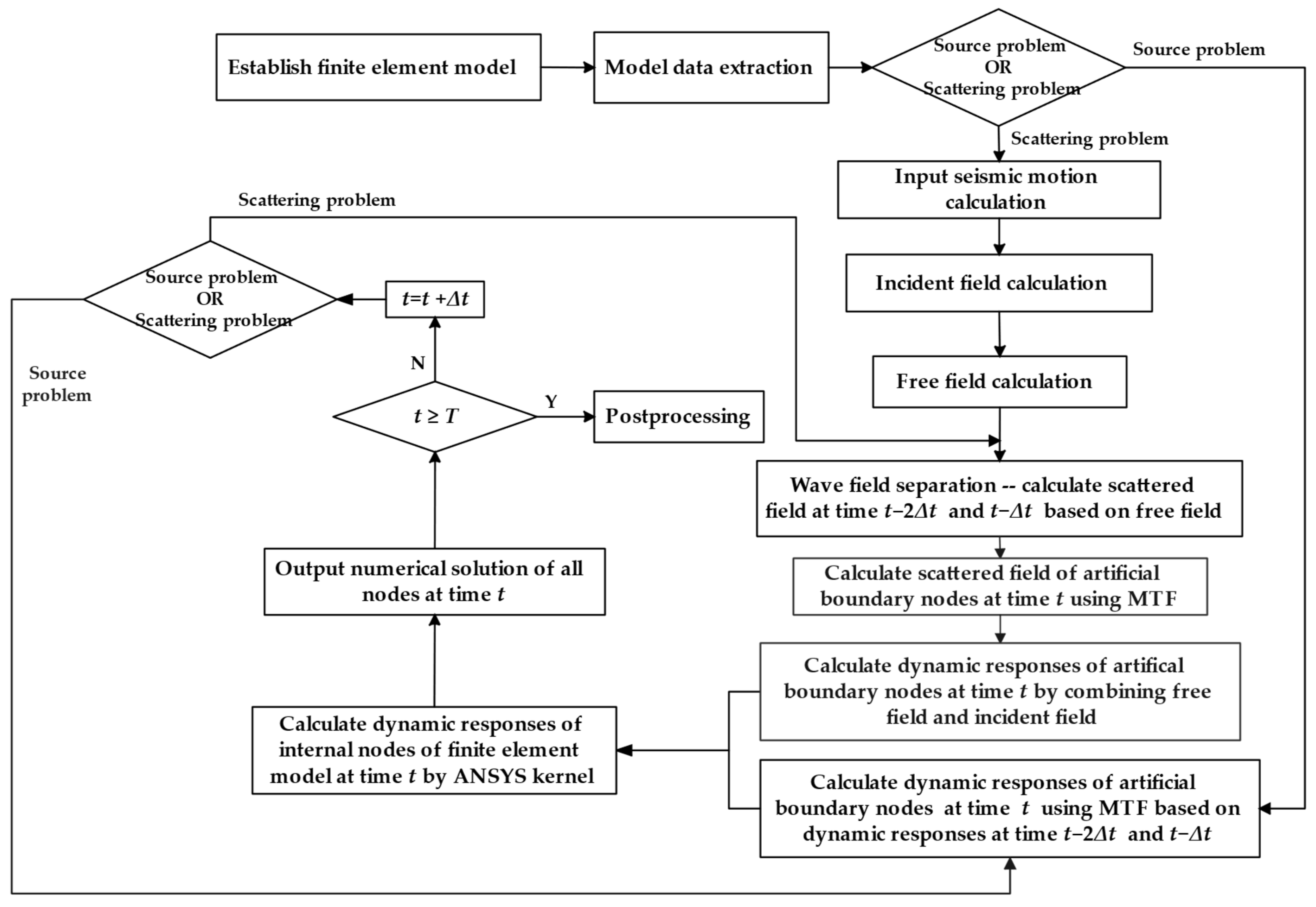
Based on the theory and physical concept of MTFs, as well as the UPFs tool provided by ANSYS, relevant user-defined subroutines were developed to accurately implement the MTF in dynamic finite element analysis within ANSYS. These user-defined subroutines perform various functions, including extracting finite element model data, calculating free field, separating wave field, computing outgoing wave field and total wave fields at artificial boundary nodes, and updating and applying boundary conditions. The flow chart of dynamic finite element analysis is presented in Figure 1, and the specific functions of each user-defined subroutine are detailed below.

(1)

Subroutine 1 extracts the finite element model data required for the MTF from the ANSYS database. These data include the IDs of each artificial boundary node and the five adjacent inner nodes along the boundary’s normal direction, the depth coordinate of each boundary node, and the relevant soil layer material parameters (e.g., shear wave velocity, density, Poisson’s ratio, damping ratio, etc.).

(2)

Subroutine 2 identifies the analysis type as either a scattering problem or a source problem. In the case of a scattering problem, the input seismic motion at each calculation time point is obtained through linear interpolation or sampling from the original seismic record. For a source problem, since there is no need to calculate the input seismic motion and free field (as the total wave field is equivalent to the scattered field), Subroutine 2 exits directly, and the ANSYS kernel proceeds to call Subroutine 5.

(3)

Subroutine 3 calculates the incident wave field at each bottom boundary node and its five adjacent inner nodes along the normal direction of the bottom boundary using plane wave propagation theory, based on the input seismic motion from Subroutine 2.

(4)

Subroutine 4 was developed to calculate the free field. It begins by establishing a one-dimensional seismic response analysis model for the soil layer, utilizing the model data extracted by Subroutine 1. The dynamic responses of this one-dimensional model to the input seismic motion provided by Subroutine 2 are then solved using the one-dimensional time domain explicit dynamic finite element method. The incident field obtained from Subroutine 3 is used to separate the scattered field from the total field at the bottom boundary node and its five adjacent inner nodes at time $\left(t-∆t\right)$, allowing for the scattered field of the bottom boundary node at time $t$ to be easily calculated using the MTF. Subsequently, the total field at the bottom boundary node at time $t$ can be obtained by superimposing the scattered field with the incident field at time $t$, thereby replacing the dynamic response of the bottom boundary node calculated by the one-dimensional time domain explicit dynamic finite element method. This iterative process continues until the free field is determined for the entire analysis period. Finally, based on the information from the artificial boundary nodes and their corresponding adjacent five inner nodes (Subroutine 1), the correspondence with the one-dimensional soil layer nodes is determined, and the free field is assigned to the finite element model. Detailed implementation methods can be found in [51].

(5)

Subroutine 5 was developed to calculate the dynamic responses of boundary nodes at time $t$ for two-dimensional or three-dimensional finite element models established in ANSYS. In the case of scattering problems, since the total field at boundary nodes and their corresponding five adjacent inner nodes along the boundary’s normal at times $\left(t-2∆t\right)$ and $\left(t-∆t\right)$ are known, the total field can be separated into scattered field at times $\left(t-2∆t\right)$ and $\left(t-∆t\right)$ by considering the free field calculated in Subroutine 4. The scattered field at the boundary nodes at time $t$ can then be calculated using the MTF. Subsequently, the total field at time $t$ can be easily determined by combining the scattered field and free field of boundary nodes at time $t$. For source problems, where the scattered field represents the total field, the total field at boundary nodes at time $t$ can be directly computed using the MTF, considering the total field of boundary nodes and their corresponding five neighboring inner nodes along the boundary’s normal at time $\left(t-2∆t\right)$ and $\left(t-∆t\right)$. Additionally, a small correction coefficient (considered in the MTF) is applied to mitigate the occurrence of low-frequency drift [9,52,53].

(6)

Subroutine 6 updates boundary constraints in ANSYS utilizing the dynamic responses of artificial boundary nodes at time $t$, which are computed from Subroutine 5 by the MTF.

All six user-defined subroutines were programmed in Fortran and integrated into ANSYS software using the UPFs tool provided by ANSYS, resulting in a customized version of ANSYS capable of performing dynamic response analysis of open systems using MTFs. These subroutines can be called via the ANSYS APDL command to implement various functions.

As illustrated in the flow chart in Figure 1, the primary purpose of Subroutine 1–Subroutine 4 is to prepare the parameters to be passed to Subroutine 5, which uses the MTF to determine the boundary conditions for the finite element model established in ANSYS. Additionally, Subroutine 1–Subroutine 4 must be executed sequentially, as the output of each subroutine serves as the foundation for the subsequent one. Based on the outputs obtained from Subroutine 1–Subroutine 4, Subroutine 5 and Subroutine 6 are then executed in a loop until the simulation is complete, enabling dynamic updating of the boundary conditions.

Figure 1. Flow chart of dynamic finite element analysis with MTF.

Figure 1. Flow chart of dynamic finite element analysis with MTF.

2.3. Determination of Element Size and Time Increment

In finite element analysis, the selection of element size and time increment is critical in ensuring the accuracy and numerical stability of the solutions. In this paper, the finite element size is determined using Equation (14).

$$∆x⩽\left({\displaystyle \frac{1}{8}}~{\displaystyle \frac{1}{6}}\right){\lambda }_{\mathrm{m}\mathrm{i}\mathrm{n}}=\left({\displaystyle \frac{1}{8}}~{\displaystyle \frac{1}{6}}\right){\displaystyle \frac{c}{f_{\mathrm{m}\mathrm{a}\mathrm{x}}}}$$

(14)

Here, $∆x$ denotes the maximum allowable finite element size, $c$ is the shear wave velocity, ${\lambda }_{\mathrm{m}\mathrm{i}\mathrm{n}}$ is the minimum wavelength, and $f_{\mathrm{m}\mathrm{a}\mathrm{x}}$ is the maximum frequency. The finite element size, as determined by Equation (14), is used to determine the critical time increment based on Equation (15) as follows:

$$∆t={\displaystyle \frac{∆x}{c}}$$

(15)

where $∆t$ denotes the critical time increment. However, to ensure computational stability and accuracy, as well as to accommodate high-frequency components, the time increment used in finite element analysis will be further reduced from $∆t$. Subsequent sections of this paper will define the element size and time increment for the finite element computational model using Equations (14) and (15).

3. Verification of MTF’s Stable Implementation in ANSYS

This section seeks to verify stable implementation of the MTF in ANSYS and evaluate its numerical accuracy using examples of a three-dimensional scattering problem and a three-dimensional source problem. The term ‘source problem’ describes scenarios in which the wave source is positioned within the computational domain, subsequently radiating energy to the infinite domain. In contrast, ‘scattering problem’ is characterized by the wave source being located outside the computational domain. When incident waves stimulate vibrations in a site or structure, the site or structure serves as a scattering wave source, radiating energy back into the infinite domain.

3.1. Scattering Problem

The scattering problem in our research pertains to the issue of seismic responses of a horizontally layered elastic half-space subjected to input seismic motion. To address this infinite domain problem, the MTF is applied at the artificial boundaries of the finite element model to simulate the effect of radiation damping in the horizontally layered elastic half-space, ensuring the unimpeded propagation of the scattered field caused by ground surface and soil layers throughout the computational domain, and eliminating any reflections at artificial boundaries.

In the context of the scattering problem, the accuracy of free field calculation is essential for ensuring accurate simulation outcomes. To verify the accuracy of free field calculation, a model of a homogeneous elastic half-space is first constructed. The input seismic motion is a semi-sinusoidal pulse with an amplitude of 1 mm and a width of 0.1 s. The normalized semi-sinusoidal pulse is illustrated in Figure 2. The seismic responses are calculated using user-defined subroutines (Subroutine 2–Subroutine 4), and the dynamic responses of the bottom boundary and free surface are presented in Figure 3. The analysis indicates that the amplitude of the free field at the bottom boundary is equivalent to that of the input seismic ground motion. At the free surface, however, the amplitude of the free field is observed to be twice that of the input seismic motion. These results demonstrate the correctness of the free field calculation, as well as verify the correctness and reliability of user-defined subroutines (Subroutine 1–Subroutine 4).

To verify the numerical solutions of the scattering problem, we developed a soil layer model in ANSYS, featuring a cubic geometry with each side uniformly measuring 10 m. The soil is stratified into three layers, and

Table 1. Media of soil layers and corresponding parameters.

No.	Soil Layer Description	Layer Thickness (m)	Shear Wave Velocity (m/s)	Density (kg/m3)	Poisson’s Ratio
1	Mud clay	2	118.3	1950	0.3
2	Silty clay	3	217.5	1790	0.3
3	Silty clay	5	254.5	1790	0.3

provides an overview of the specific parameters for each soil layer. Considering the accuracy requirements for dynamic finite element analysis, the mesh size was set to 0.5 m. Based on this, the model was spatially discretized, and the dynamic finite element motion equations of internal nodes were established, which are solved by ANSYS kernel, while the dynamic responses of artificial boundary nodes are calculated using the MTF (Subroutine 5 and Subroutine 6). The time increment, $∆t$, was determined to be 0.0004 s based on the effective frequency band of the input seismic motion and the stability requirements. The input seismic motion, shown in Figure 2, was uniformly input from the bottom boundary, with vibrations occurring along the horizontal axis. The total calculation duration is 0.6 s.

According to wave theory, if the medium is layered and subjected to a perpendicularly incident plane wave, the problem can typically be simplified to a one-dimensional problem along the vertical (depth) direction. Based on the steady-state wave-motion analytical solution of the horizontally stratified medium [54], a program was developed with Fortran to analyze the dynamic responses of layered soil under vertically incident seismic waves. This result can serve as the analytical solution for the scattering problem in this subsection. Thus, stable implementation of the MTF in ANSYS and the accuracy of the numerical solution can be verified by comparing with the analytical solution. The numerical solution and corresponding analytical solution at the bottom boundary and free surface are presented in Figure 4a,b, respectively. It can be observed that the numerical solutions align closely with the analytical solutions, demonstrating that the MTF was successfully integrated into ANSYS with high computational accuracy and numerical stability. From Figure 4, it can also be shown that the MTF ensures the scattered waves pass through artificial boundaries without energy reflection. Thus far, the case study verified the correctness of Subroutine 5 and Subroutine 6 and the successful integration of the MTF into ANSYS as a local artificial boundary condition for dynamic finite element analysis of open systems.

3.2. Source Problem

In Section 3.1, successful integration of the MTF into ANSYS with high computational accuracy and numerical stability was verified through a 3D scattering problem. Moreover, this subsection extends the verification by applying the MTF to a 3D source problem. Additionally, this subsection compares the numerical solutions obtained using the MTF as a boundary condition with the numerical solutions of other commonly used artificial boundary conditions in finite element simulations, highlighting the advantages of using MTFs.

In the source problem, the scattered field is equivalent to the total field, allowing the straightforward calculation of dynamic responses of boundary nodes using MTFs without the need for wave field separation. The finite element model used in the source problem is identical to that established in the scattering problem. Additionally, a semi-sinusoidal vertical downward pulse force with a duration of 0.1 s and an amplitude of 10⁸ N was applied at the center of the top boundary (free surface). The meshing strategy and analysis settings remain consistent with those outlined in Section 3.1. The numerical simulation result is shown in Figure 5 as a solid black line, while the numerical solutions for the viscous boundary and viscous-spring boundary are also provided in Figure 5 as dotted lines.

Additionally, in order to compare the impact of different artificial boundary conditions on the accuracy of dynamic finite element simulation, a model whose boundary condition is a remote boundary was also established. To ensure the reliability of dynamic response analysis, the remote boundary must guarantee that the reflected wave energy from the boundary does not affect the structural response during the analysis. Hence, the size of the model is determined according to Equation (16) [18] as follows:

$$L⩾2\times T\times C$$

(16)

where $L$ is the distance from the boundary to the location of the scattered source, $T$ is the analysis duration, and $C$ is the shear wave velocity in the soil medium. Based on this, in this subsection, the size of the model with the remote boundary was set as 50 m × 50 m × 50 m, and the mesh size was still set to 0.5 m. The numerical solution for the remote boundary is also presented in Figure 5 as an accurate solution.

Figure 5 demonstrates the presence of numerical drift in the results obtained using the viscous boundary, which is inconsistent with qualitative analysis expectations. Although the viscous-spring boundary overcomes this shortcoming, noticeable repeated oscillations persist due to boundary reflections. Moreover, the stiffness parameter of the viscous-spring boundary is related to the distances ($R$) between the boundary nodes and scattering sources, and the appropriateness of this parameter influences the numerical solutions. Nevertheless, the distance $R$ is primarily determined empirically. In contrast to the previously mentioned artificial boundaries, the MTF is not highly sensitive to its sole parameter—artificial wave velocity ($c_a$). Compared with the numerical solution for the remote boundary, the dynamic response obtained using the MTF is very close, without issues of numerical drift or oscillation caused by energy reflection at artificial boundaries, and the computation time is also significantly shorter. Consequently, the MTF-based numerical simulation results exhibit high numerical accuracy and stability, and the performance of the MTF in dynamic finite element analysis of open systems is superior to that of other artificial boundary conditions.

4. Field Observation and Analysis of Railway-Induced Environmental Vibration

4.1. Field Observation

To investigate the effects of railway-induced environmental vibration, a series of field observations were carried out. Nine observation sites were selected along the Beijing–Shanghai high-speed railway: Dezhou, Zaozhuang, Jining, Xuzhou, Suzhou, Chuzhou, Nanjing, Wuxi, and Kunshan. The selection of these observation sites was based on the fundamental principle of maximizing flat and open terrain, with no nearby buildings or traffic facilities to minimize interference. Three-component vibration acceleration was recorded at depths of 0 m, 1 m, 2 m, 3 m, and 5 m beneath the surface for analysis.

The ETNA2 equipment (Kinemetrics Inc., Pasadena, CA, USA) (Figure 6) was employed for recording vibration acceleration. It is a 3-channel 24-bit digital strong motion accelerometer that offers multiple advantages, such as cost-effectiveness, wide frequency bandwidth, low noise level and high resolution. In addition, it features trigger recording, continuous recording, timing recording, and automatic GPS timing functionalities, facilitating the efficient collection of time history data for three-component acceleration. Prior to conducting on-site observations, we thoroughly calibrated all ETNA2 to ensure the accuracy of the data collected.

However, during the data analysis, we discovered significant differences in the vibration attenuation characteristics along the depth direction between the Kunshan site and the other sites. The acceleration time histories at depths of 0 m, 1 m, 2 m, 3 m, and 5 m beneath the ground surface are depicted in Figure 7. It should be noted that in Figure 7, the ‘perpendicular’ refers to the horizontal direction orthogonal to the railway track extension, designated as the y-direction. Additionally, the ‘vertical’ aligns with the depth of the soil, indicated as the z-direction, while ‘parallel’ corresponds to the direction along the railway track, which is the x-direction. The data serve as the basis for illustrating the relationship between three-component peak acceleration and depth, depicted in Figure 8. Notably, the vibration intensity does not exhibit a gradual decrease with increasing depth, but rather shows significant amplification relative to the ground surface within a specific depth range across all three components [55].

The subgrade of the Kunshan segment of the Beijing–Shanghai high-speed railway is a viaduct. Vibrations generated by high-speed train operations propagate through the subsoil via bridge piers and pile foundations, inducing environmental vibrations along the railway lines. Analysis of borehole data from the Kunshan observation site revealed the presence of a 3-m-thick layer of mud clay situated 2 m beneath the ground surface. Preliminary qualitative analysis suggests that the presence of the mud clay layer may contribute to vibration amplification at a specific depth.

4.2. Numerical Analysis

To validate the qualitative analysis, two horizontally layered three-dimensional finite element models were established based on the borehole data from the Kunshan observation site. One model includes piles, while the other does not. Figure 9 illustrates the schematic diagram of the model with piles, with dimensions of 10 m × 10 m × 17 m. The piles measure 2 m × 2 m × 15 m and are spaced 2 m apart. The piles possess an elastic modulus of 2.6 × 10⁴ MPa, a Poisson’s ratio of 0.167, and a density of 2500 kg/m³. The parameters of the subsoils are provided in

Table 2. Media of finite element model and their parameters.

No.	Soil Properties	Layer Bottom Depth (m)	Layer Thickness (m)	Shear Wave Velocity vs (m/s)	Density (t/m3)
①	Silty clay	2	2	245.0	1.79
②	Mud clay	5	3	100.0	1.95
③	Silty clay	8	3	217.5	1.79
④	Silty clay	12	4	254.5	1.79
⑤	Silty soil	17	5	391.0	1.87

. Both the subsoils and piles were discretized using 3D solid elements with a mesh size of 0.25 m to meet the accuracy requirements for dynamic finite element analysis. This section primarily focuses on exploring the attenuation patterns of environmental vibrations induced by high-speed railway trains. Therefore, the interaction between the trains and bridges is simplified. Six downward semi-sinusoidal pulses, with an amplitude of 10⁵ N and a duration of 0.05 s, were applied to the top center of each pile, as shown in Figure 10, with each pulse separated by a time interval of 0.002 s, corresponding to a high-speed train speed of 300 km/h. The motion equations for the internal nodes were established, which are solved by ANSYS kernel, while the dynamic responses of artificial boundary nodes were calculated using the MTF. The time increment, $∆t$, was set to 0.0002 s based on the effective frequency bandwidth of the input loads and the accuracy requirements for the analysis. The total duration of the simulation was set to 0.3 s. Additionally, Rayleigh damping was considered. In the numerical analysis, five observation locations were selected on the ground surface, with 13 observation points arranged at various depths (0.0 m, 1.0 m, 2.0 m, 3.0 m, 3.5 m, 4.0 m, 4.5 m, 5.0 m, 6.0 m, 7.0 m, 8.0 m, 9.0 m, and 10.0 m) for each observation location, as shown in Figure 9. The model without piles uses the same subsoil parameters, geometry size, finite element size, damping parameters, applied loads, and observation point layout as the model with piles. Figure 11 displays the variations in vertical peak acceleration as the depth increases at observation location 1 for both models, while Figure 12 shows the variations in vertical peak acceleration with depth at all observation locations in the model with piles.

Figure 11 illustrates that the attenuation behavior of peak accelerations in the presence of piles (black line) differs significantly from that in the absence of piles (red line) as the depth increases. Furthermore, peak accelerations at different depths in the model with piles are significantly lower than those in the model without piles. Qualitatively speaking, when the loads are applied to the top surface of the piles, the majority of the energy is transmitted through the piles, with only a small portion of wave energy entering the shallow subsoils, while a larger portion is directly transmitted into deep subsoils through the piles. In contrast, all the energy diffuses through the shallow subsoils in the model without piles. Thus, the vibration intensity in the case without piles is higher. In the case with piles, the peak acceleration exhibits a slight attenuation from 0 m to 2 m. However, significant amplification occurs within the mud clay, reaching its highest value at a depth of 3.5 m, surpassing even that of the ground surface. Subsequently, the peak acceleration gradually decreases with increasing depth. Comparing the attenuation characteristics of the numerical simulation results with those of the data at the Kunshan observation site reveals a strong similarity. Therefore, when piles and the underlying mud clay coexist, peak vibration accelerations in the mud clay will undergo significant amplification.

As shown in Figure 12, for the model with piles, the trend of peak acceleration with increasing depth at observation location 2 to 5 is similar to that at observation location 1, with the only difference being that peak acceleration decreases and converges at the same depth as the distance from the load-applied points increases.

In comparison to the results of the model with piles, the model without piles shows no vibration amplification, suggesting that piles play a crucial role in the amplification of peak acceleration in the underlying soft soil layer. In the presence of piles, the vibration energy generated by high-speed trains is directly transmitted through the piles into the soil layers beneath the soft soil layer, resulting in a proportion of vibration energy propagating upward. The vibration energy is then amplified within the soft soil layer and compounded by the vibration energy transmitted from the ground surface, further amplifying the acceleration within the soft soil layer. Therefore, the significant amplification of peak acceleration in the mud clay layer is due to the combined effect of piles and the soft clay layer.

This case study reveals the amplification mechanism of peak acceleration induced by high-speed trains in mud clay. Furthermore, the influence of piles on vibration intensity characteristics is also demonstrated. It can be concluded that the combined effect of piles and subsoils can effectively reduce vibration intensity at nearby sites along railway lines induced by high-speed train operation.

5. Conclusions

In this paper, an MTF was integrated into ANSYS software through secondary development by the UPFs tool so that it could be applied in dynamic finite element analysis of open systems as an artificial boundary condition. The high simulation accuracy and numerical stability of the MTF were verified through a 3D scattering problem and a 3D source problem. The conclusions are as follows:

(1)

The MTF exhibits high computational accuracy. In the scattering problem, its numerical solutions match the analytical solution well based on the layered steady-state wave theory, while in the source problem, its results align closely with those obtained using the remote boundary.

(2)

The performance of the MTF in dynamic finite element analysis of open systems is superior to that of other artificial boundary conditions, such as viscous boundary and viscous-spring boundary, without numerical drift or oscillation caused by energy reflection at artificial boundaries.

Moreover, in order to investigate the propagation patterns and mechanisms of environmental vibrations induced by train operations on elevated railway sections with underlying soft soil layers, field observation and numerical simulation were conducted, and the results exhibit strong similarity. The main conclusions are listed below.

(1)

The significant amplification of peak acceleration in the mud clay layer is due to the combined effect of piles and the soft clay layer. The vibration energy is directly transmitted through the piles into soil layers under the soft soil layer. Some of the energy propagates upward and amplifies within the soft soil layer, compounded by vibrations from the ground surface, resulting in further amplification.

(2)

The combined effect of piles and subsoils can effectively reduce vibration intensity at nearby sites along railway lines induced by high-speed train operation.

References

1. Yang, Y.; Li, J.; Wu, W. Modeling Wave Propagation across Rock Masses Using an Enriched 3D Numerical Manifold Method. Sci. China Technol. Sci. 2024, 67, 835–852. [Google Scholar] [CrossRef]
2. Chen, W.Y. Analysis of Dynamic Characteristics of Pile-Soil Coupling Effect in Consideration of Large Span Cable-Stayed Bridge. Appl. Mech. Mater. 2014, 501–504, 1270–1273. [Google Scholar] [CrossRef]
3. Cen, H.; Zong, Z.; Huang, D.; Wang, H.; Zhuang, X.; Huang, Z.; Tang, A. Study of the Dynamic Interactions between Helix-Stiffened Cement Mixing Piles and Soft Soil under Oblique Incidence of SV Waves in Arbitrary Space. Comput. Geotech. 2024, 171, 106388. [Google Scholar] [CrossRef]
4. Li, M.; Meng, K.; Zhou, J.; Zhang, J.; Zhong, G.; Song, S. Seismic Response and Damage Analysis of Shield Tunnel with Bottom Karst Caves under Oblique SV Waves. Nat. Hazards 2024, 120, 2731–2747. [Google Scholar] [CrossRef]
5. Su, J.; Zhou, Z.; Li, Y.; Hao, B.; Dong, Q.; Li, X. A Stable Implementation Measure of Multi-Transmitting Formula in the Numerical Simulation of Wave Motion. PLoS ONE 2020, 15, e0243979. [Google Scholar] [CrossRef]
6. Tang, H.; Rong, M.-S. An Improved Wave Motion Input Method for Application of Multi-Transmitting Boundary. Wave Motion 2020, 97, 102600. [Google Scholar] [CrossRef]
7. Xing, H.; Li, X.; Li, H.; Liu, A. Spectral-Element Formulation of Multi-Transmitting Formula and Its Accuracy and Stability in 1D and 2D Seismic Wave Modeling. Soil. Dyn. Earthq. Eng. 2021, 140, 106218. [Google Scholar] [CrossRef]
8. Xing, H.; Li, X.; Li, H.; Xie, Z.; Chen, S.; Zhou, Z. The Theory and New Unified Formulas of Displacement-Type Local Absorbing Boundary Conditions. Bull. Seismol. Soc. Amer 2021, 111, 801–824. [Google Scholar] [CrossRef]
9. Yang, Y.; Li, X.; Rong, M.; Yang, Z. Strategy for Eliminating High-Frequency Instability Caused by Multi-Transmitting Boundary in Numerical Simulation of Seismic Site Effect. Front. Earth Sci. 2022, 10, 1056583. [Google Scholar] [CrossRef]
10. Yu, Y.; Ding, H.; Zhang, X. Formulation and Performance of Multi-Transmitting Formula with Spectral Element Method in 2D Ground Motion Simulations Under Plane-Wave Incidence: SV Wave Problem. J. Earthq. Eng. 2024, 28, 1837–1860. [Google Scholar] [CrossRef]
11. Haji, T.K.; Faramarzi, A.; Metje, N.; Chapman, D.; Rahimzadeh, F. Development of an Infinite Element Boundary to Model Gravity for Subsurface Civil Engineering Applications. Int. J. Numer. Anal. Methods Geomech. 2020, 44, 418–431. [Google Scholar] [CrossRef]
12. Khalil, A.E.; Hameed, M.F.O.; Obayya, S.S.A. Leaky Mode Analysis Using Complex Infinite Elements. Opt. Quantum Electron. 2024, 56, 106. [Google Scholar] [CrossRef]
13. Dastour, H.; Liao, W. A Fourth-Order Optimal Finite Difference Scheme for the Helmholtz Equation with PML. Comput. Math. Appl. 2019, 78, 2147–2165. [Google Scholar] [CrossRef]
14. Kumar, R.; Sharma, A. Absorbing Boundary Condition (ABC) and Perfectly Matched Layer (PML) in Numerical Beam Propagation: A Comparison. Opt. Quantum Electron. 2019, 51, 53. [Google Scholar] [CrossRef]
15. Zhuang, M.; Zhan, Q.; Zhou, J.; Guo, Z.; Liu, N.; Liu, Q.H. A Simple Implementation of PML for Second-Order Elastic Wave Equations. Comput. Phys. Commun. 2020, 246, 106867. [Google Scholar] [CrossRef]
16. Wang, Y.; Zhou, M.; Cao, Y.; Wang, X.; Li, Z.; Ma, M. Simplified Tunnel–Soil Model Based on Thin-Layer Method–Volume Method–Perfectly Matched Layer Method. Appl. Sci. 2024, 14, 5692. [Google Scholar] [CrossRef]
17. Ya, R.; Wu, J.; Tang, R.; Yang, Y.; Wang, L. Multi-Hazard Direct Economic Loss Risk Assessment on the Tibet Plateau. Geomat. Nat. Hazards Risk 2024, 15, 2368075. [Google Scholar] [CrossRef]
18. Ding, Z.; Chen, Y.; Zi, H. Study on Artificial Boundary and Ground Motion Input Method in Tunnel Seismic Response. Earthq. Eng. Eng. Dyn. 2022, 42, 52–61. [Google Scholar] [CrossRef]
19. Yu, H.; Wang, Z. Efficient Hybrid Simulation Method for Seismic Response Analysis of Underground Structures. Chin. J. Geotech. Eng. 2024, 46, 45–53. [Google Scholar]
20. Zhao, C. Coupled Method of Finite and Dynamic Infinite Elements for Simulating Wave Propagation in Elastic Solids Involving Infinite Domains. Sci. China Technol. Sci. 2010, 53, 1678–1687. [Google Scholar] [CrossRef]
21. Xu, G.; Duan, W.-Y. Time-Domain Simulation of Wave–Structure Interaction Based on Multi-Transmitting Formula Coupled with Damping Zone Method for Radiation Boundary Condition. Appl. Ocean Res. 2013, 42, 136–143. [Google Scholar] [CrossRef]
22. Yu, Y.; Ding, H.; Zhang, X. Simulations of Ground Motions under Plane Wave Incidence in 2D Complex Site Based on the Spectral Element Method (SEM) and Multi-Transmitting Formula (MTF): SH Problem. J. Seismolog. 2021, 25, 967–985. [Google Scholar] [CrossRef]
23. Shi, L.; He, J.; Huang, Z.; Sun, H.; Yuan, Z. Numerical Investigations on Influences of Tunnel Differential Settlement on Saturated Poroelastic Ground Vibrations and Lining Forces Induced by Metro Train. Soil. Dyn. Earthq. Eng. 2022, 156, 107202. [Google Scholar] [CrossRef]
24. Jirong, S.; Shaolin, C.; Jiao, Z.; Puxin, C. Unified Framework Based Parallel FEM Code for Simulating Marine Seismoacoustic Scattering. Front. Earth Sci. 2023, 10, 1056485. [Google Scholar] [CrossRef]
25. Xie, Z.; Zhang, X. Analysis of High-Frequency Local Coupling Instability Induced by Multi-Transmitting Formula–P-SV Wave Simulation in a 2D Waveguide. Earthq. Eng. Eng. Vib. 2017, 16, 1–10. [Google Scholar] [CrossRef]
26. Di, G.; Xie, Z.; Guo, J. Predict the Influence of Environmental Vibration from High-Speed Railway on Over-Track Buildings. Sustainability 2021, 13, 3218. [Google Scholar] [CrossRef]
27. Zhang, Y.; Lou, Y.; Zhang, N.; Cao, Y.; Chen, L. Attenuation and Prediction of the Ground Vibrations Induced by High-Speed Trains Running Over Bridge. Int. J. Struct. Stab. Dyn. 2021, 21, 2150076. [Google Scholar] [CrossRef]
28. Çelebi, E.; Zülfikar, A.C.; Göktepe, F.; Kırtel, O.; Faizan, A.A.; İstegün, B. In-Situ Measurements and Data Analysis of Environmental Vibrations Induced by High-Speed Trains: A Case Study in North-Western Turkey. Soil. Dyn. Earthq. Eng. 2022, 156, 107211. [Google Scholar] [CrossRef]
29. Faizan, A.A.; Kırtel, O.; Çelebi, E.; Zülfikar, A.C.; Göktepe, F. Experimental Validation of a Simplified Numerical Model to Predict Train-Induced Ground Vibrations. Comput. Geotech. 2022, 141, 104547. [Google Scholar] [CrossRef]
30. Zheng, H.; Yan, W. Field and Numerical Investigations on the Environmental Vibration and the Influence of Hill on Vibration Propagation Induced by High-Speed Trains. Constr. Build. Mater. 2022, 357, 129378. [Google Scholar] [CrossRef]
31. Niu, D.; Deng, Y.; Mu, H.; Chang, J.; Xuan, Y.; Cao, G. Attenuation and Propagation Characteristics of Railway Load-Induced Vibration in a Loess Area. Transp. Geotech. 2022, 37, 100858. [Google Scholar] [CrossRef]
32. Wang, C.; Lei, X.; Wang, P.; Liu, W. Study of Ground Vibration Caused by High-Speed Trains Through Bridges Based on Finite Element Model: Test Validation. KSCE J. Civ. Eng. 2024, 28, 3758–3767. [Google Scholar] [CrossRef]
33. Zheng, H.; Yan, W. Experimental and Numerical Studies on Environmental Vibration Characteristics of Pier and Foundation Sites Caused by High-Speed Trains in Seasonally Frozen Regions. Acta Geotech. 2024, 19, 305–326. [Google Scholar] [CrossRef]
34. İstegün, B.; Çelebi, E.; Kırtel, O.; Faizan, A.A.; Göktepe, F.; Zülfikar, A.C.; Subaşı, A.; Navdar, M.B. Mitigation of High-Speed Train-Induced Environmental Ground Vibrations Considering Open Trenches in the Soft Soil Conditions by in-Situ Tests. Transp. Geotech. 2023, 40, 100980. [Google Scholar] [CrossRef]
35. Auersch, L. Reduction of Train-Induced Vibrations—Calculations of Different Railway Lines and Mitigation Measures in the Transmission Path. Appl. Sci. 2023, 13, 6706. [Google Scholar] [CrossRef]
36. Çelebi, E.; Kırtel, O.; İstegün, B.; Göktepe, F.; Burhan Navdar, M.; Subaşı, A.; Can Zülfikar, A. Mitigation of High-Speed Train Induced Surface Vibrations by Open Trench with Aerated Concrete Panel Walls. Constr. Build. Mater. 2023, 400, 132771. [Google Scholar] [CrossRef]
37. Barman, R.; Sarkar, A.; Bhowmik, D. Composite Sand-Crumb Rubber and Geofoam Wave Barrier for Train Vibration. Geotech. Geol. Eng. 2024, 42, 2321–2343. [Google Scholar] [CrossRef]
38. Çelebi, E.; Kırtel, O.; İstegün, B.; Navdar, M.B.; Subaşı, A.; Göktepe, F.; Zülfikar, A.C. High-Speed Train Induced Environmental Vibrations: Experimental Study on Isolation Efficiency of Recyclable in-Filling Materials for Thin-Walled Hollow Wave Barrier. Eng. Struct. 2024, 312, 118207. [Google Scholar] [CrossRef]
39. Coulier, P.; Hunt, H.E.M. Experimental Study of a Stiff Wave Barrier in Gelatine. Soil. Dyn. Earthq. Eng. 2014, 66, 459–463. [Google Scholar] [CrossRef]
40. Dijckmans, A.; Ekblad, A.; Smekal, A.; Degrande, G.; Lombaert, G. Efficacy of a Sheet Pile Wall as a Wave Barrier for Railway Induced Ground Vibration. Soil. Dyn. Earthq. Eng. 2016, 84, 55–69. [Google Scholar] [CrossRef]
41. Andersen, L.; Nielsen, S.R.K. Reduction of Ground Vibration by Means of Barriers or Soil Improvement along a Railway Track. Soil. Dyn. Earthq. Eng. 2005, 25, 701–716. [Google Scholar] [CrossRef]
42. Dijckmans, A.; Coulier, P.; Jiang, J.; Toward, M.G.R.; Thompson, D.J.; Degrande, G.; Lombaert, G. Mitigation of Railway Induced Ground Vibration by Heavy Masses next to the Track. Soil. Dyn. Earthq. Eng. 2015, 75, 158–170. [Google Scholar] [CrossRef]
43. Gao, G.; Li, N.; Gu, X. Field Experiment and Numerical Study on Active Vibration Isolation by Horizontal Blocks in Layered Ground under Vertical Loading. Soil. Dyn. Earthq. Eng. 2015, 69, 251–261. [Google Scholar] [CrossRef]
44. Gao, G.; Zhang, Q.; Chen, J.; Chen, Q. Field Experiments and Numerical Analysis on the Ground Vibration Isolation of Wave Impeding Block under Horizontal and Rocking Coupled Excitations. Soil. Dyn. Earthq. Eng. 2018, 115, 507–512. [Google Scholar] [CrossRef]
45. Gao, M.; Tian, S.P.; Wang, Y.; Chen, Q.S.; Gao, G.Y. Isolation of Ground Vibration Induced by High Speed Railway by DXWIB: Field Investigation. Soil. Dyn. Earthq. Eng. 2020, 131, 106039. [Google Scholar] [CrossRef]
46. Tsai, P.; Feng, Z.; Jen, T. Three-Dimensional Analysis of the Screening Effectiveness of Hollow Pile Barriers for Foundation-Induced Vertical Vibration. Comput. Geotech. 2008, 35, 489–499. [Google Scholar] [CrossRef]
47. Liu, X.; Shi, Z.; Mo, Y.L. Comparison of 2D and 3D Models for Numerical Simulation of Vibration Reduction by Periodic Pile Barriers. Soil. Dyn. Earthq. Eng. 2015, 79, 104–107. [Google Scholar] [CrossRef]
48. Li, Z.; Ma, M.; Liu, K.; Jiang, B. Performance of Rubber-Concrete Composite Periodic Barriers Applied in Attenuating Ground Vibrations Induced by Metro Trains. Eng. Struct. 2023, 285, 116027. [Google Scholar] [CrossRef]
49. Wu, L.; Shi, Z. Feasibility of Vibration Mitigation in Unsaturated Soil by Periodic Pile Barriers. Comput. Geotech. 2023, 164, 105798. [Google Scholar] [CrossRef]
50. Coulier, P.; François, S.; Degrande, G.; Lombaert, G. Subgrade Stiffening next to the Track as a Wave Impeding Barrier for Railway Induced Vibrations. Soil. Dyn. Earthq. Eng. 2013, 48, 119–131. [Google Scholar] [CrossRef]
51. Li, S.; Liao, Z.; Zhou, Z. Wave Motion Input in Numerical Simulation of Seismic Response for Large-scale Structure. Earthq. Eng. Eng. Vib. 2001, 21, 1–5. [Google Scholar] [CrossRef]
52. Zhou, Z.; Liao, Z. A Measure for Eliminating Drift Instability of the Multi-transmitting Formula. Acta Mech. Sin. 2001, 33, 550–554. [Google Scholar]
53. Tang, H.; Li, X. Analysis of Measures of Eliminating Drift Instability of Multi-transmission Formula in Solving Scattering Problem. J. Seismol. Res. 2019, 42, 493–502+649. [Google Scholar]
54. Yang, G.; Liao, Z. Finite Element Simulation of Steady Wave Motion in the Visco-elastic Layered Medium. Rock Soil Mech. 1993, 14, 41–48. [Google Scholar] [CrossRef]
55. Liu, H.; Zhou, Y.; Zhong, K.; Zhou, Z.; Li, Y.; Dong, Q.; Wang, W.; Song, J. Variation Characteristics of Foundation Soil Vibaration Caused by High speed Train with Depth under Different Site Conditions. Technol. Earthq. Disaster Prev. 2018, 13, 893–902. [Google Scholar] [CrossRef]
Figure 2. The time history of input seismic ground motion.
Buildings 14 02575 g002
Figure 3. Seismic responses of homogeneous elastic half-space site.
Buildings 14 02575 g003
Figure 4. Comparison between numerical solution and analytical solution: (a) Bottom boundary; (b) free surface (top surface).
Buildings 14 02575 g004
Figure 5. Comparison among numerical simulation results of different artificial boundaries.
Buildings 14 02575 g005
Figure 6. ETNA2 accelerometer.
Buildings 14 02575 g006
Figure 7. Acceleration time histories of three-component vibrations at different depths in Kunshan test site: (a) Depth = 0 m; (b) depth = 1 m; (c) depth = 2 m; (d) depth = 3 m; (e) depth = 5 m.
Buildings 14 02575 g007aBuildings 14 02575 g007b
Figure 8. Peak acceleration variations with depth increasing at Kunshan test site.
Buildings 14 02575 g008
Figure 9. Schematic diagram of model with piles.
Buildings 14 02575 g009
Figure 10. Applied load.
Buildings 14 02575 g010
Figure 11. Variations in vertical peak acceleration with depth at observation location 1 for both models.
Buildings 14 02575 g011
Figure 12. Variations in vertical peak acceleration with depth at all observation locations in the model with piles.
Buildings 14 02575 g012