Application of an Improved Method Combining Machine Learning–Principal Component Analysis for the Fragility Analysis of Cross-Fault Hydraulic Tunnels

Abstract

Machine learning (ML) approaches, widely used in civil engineering, have the potential to reduce computing costs and enhance predictive capabilities. However, many ML methods have yet to be applied to develop models that accurately analyze the nonlinear dynamic response of cross-fault hydraulic tunnels (CFHTs). To predict CFHT models and fragility curves effectively, we identify the most effective ML techniques and improve prediction capacity and accuracy by initially creating an integrated multivariate earthquake intensity measure (IM) from nine univariate earthquake IMs using principal component analysis. Structural reactions are then performed using incremental dynamic analysis by a multimedium-coupled interaction system. Four techniques are used to test ML–principal component analysis (PCA) feasibility. Meanwhile, mathematical statistical parameters are compared to standard probabilistic seismic demand models of expected and computed values using ML-PCA. Eventually, multiple stripe analysis–maximum likelihood estimation (MSA-MLE) is applied to assess the seismic performance of CFHTs. This study highlights that the Gaussian process regression and integrated IM can improve reliable probability and reduce uncertainties in evaluating the structural response. Thorough numerical analysis, using the suggested methodology, one can efficiently assess the seismic fragilities of the tunnel by the predicted model. ML-PCA techniques can be viewed as an alternate strategy for seismic design and CFHT performance enhancement in real-world engineering.

1. Introduction

Governments have initiated large water diversion projects to address the water supply–demand balance, critical to national infrastructure. Hydraulic tunnels (HTs) play a key role in these efforts by overcoming topographical challenges and shortening long-distance water diversions. However, these tunnels face stricter seismic design regulations, especially in high-intensity seismic zones where many natural engineering sites are located. This is particularly evident in tunnels that cross rivers and mountains. Large earthquakes have historically caused significant damage to many tunnels, especially those situated in fault fracture zones. For instance, the Chi-Chi earthquake severely displaced the Dagang HT, moving it 180 m below the tunnel water intake of a hydropower plant [1]. Various case studies [2,3,4,5,6] indicate that adverse seismic events have led to improvements in the seismic resistance of cross-fault (CF) HTs over time. Ensuring the performance of CFHTs during seismic events is crucial in active seismic locations.

With the widespread application of fragility analysis in performance-based earthquake engineering, various analytical methods such as cloud analysis incremental dynamic analysis [7], multiple stripe analysis (MSA) [8,9], and loud analysis [10], have gained popularity as essential tools for developing reliable seismic fragility curves. These approaches are crucial for establishing the seismic intensity measure (IM) that best suits the given scenario. Deriving the statistical seismic IM–demand measure (DM) relationship necessitates a large dataset of structural response findings, a prerequisite shared by the three commonly employed analytical methods [11]. To obtain the engineering demand parameters (EDPs) of subterranean structures directly, numerous nonlinear time history finite element (FE) simulations employ a suite of ground motions (GMs). However, dynamic analysis demands significant computational effort and time, rendering it impractical and inefficient [12]. To address these challenges, it is customary to utilize the methodology proposed by Baker [7] for constructing appropriate probabilistic seismic demand models (PSDMs) for subterranean structures. Computational costs are mitigated by employing a simple linear regression of the IMs-DMs relationship in logarithmic space. The primary sources of inaccuracy in seismic fragility analysis stem from the linear relationship between IM-EDP in logarithmic space and the normal distribution assumption of the structural response. Moreover, severe GM excitation induces nonlinear behavior in a structure, diminishing the effectiveness of a simplistic linear regression.

In modern civil engineering problems, data-driven machine learning (ML) approaches are being used more and more as a viable alternative to reduce the computational load in seismic safety assessment, which can improve computer efficiency by adjusting the statistical relationship between seismic inputs and EDPs [13,14,15,16]. Kiani et al. [12] implemented ML tools into the performance-based earthquake engineering of a steel moment resisting frame for estimating the seismic resistance of the structure, which demonstrated that the random forest (RF) method had the optimal performance for predicting structural performance. Jeddi et al. [17] used support vector machine (SVM) and fragility analysis to analyze the earthquake resistance of concrete-faced rockfill dams subjected to one hundred artificial. They found that SVM algorithms have the potential to improve the computational efficiency of FEM. Liu and Macedo [18] investigated the reliability of PSDM of the gradient-boosting decision tree, RF, and residual NNs for slopes according to the prediction error and computational cost. The proposed models demonstrated superior predictive capabilities on test sets compared with traditional proxies. Wang et al. [4] found the prediction accuracy of the EDP of nuclear power plants by artificial NNs is higher than the traditional method. Numerous studies have also shown that employing ML algorithms to anticipate structural reactions is more reliable and effective than using the conventional assumption method when evaluating the seismic performance of above-ground structures [19,20,21,22,23,24,25]. However, there is a shortage of research on the utilization of ML algorithms for evaluating the seismic performance of HTs. Consequently, more research is required to utilize ML’s full potential in assisting engineers and decision-makers in taking the necessary preventive actions against the likely outcomes of HT failure.

On the other hand, establishing the IMs-DMs relationship of ML algorithms requires the appropriate form of IM, which can effectively represent the essential features of strong GMs and accurately correlate with the structural response. Moreover, it can reduce uncertainties and enhance the accuracy in assessing the structural response. Obviously, the optimal choice of IMs for various underground structures has attracted extensive attention from researchers in the past decade [26,27,28,29]. However, most of the previous studies have a common characteristic that focuses on the selection of scalar-valued IMs. It is well-known that different IMs of seismic GMs represent different seismology features of GMs, and the selection of multiple IMs is critical for accurate seismic hazard assessment and engineering design [30]. As a result, it is difficult to create several IMs that accurately convey GM uncertainty and reflect more seismology properties.

In light of the significance of HTs in hydraulic engineering and civil engineering, the efficient implementation of PSDMs for seismic fragility analysis is in its preliminary stage. Accordingly, this research aims to investigate the copulating method with principal component analysis (PCA) and ML to improve the reliability and application of seismic fragility analysis for HTs. This manuscript is structured as follows: Section 2 outlines a powerful dimension-reduction method (PCA) for intensity measures. Section 3 provides a concise overview of ML, while Section 4 elucidates the fragility analysis approach based on maximum likelihood estimation (MLE) and MSA. The synthesis of combined intensity measures by PCA and adjusted GMs by the increment dynamic analysis method is detailed in Section 5. Section 6 introduces an FE numerical model for CFHTs, incorporating a multi-medium-coupled interaction system to predict structural responses. Subsequently, Section 7 presents the analysis and discussion, culminating in concluding remarks derived from the findings (Section 8).

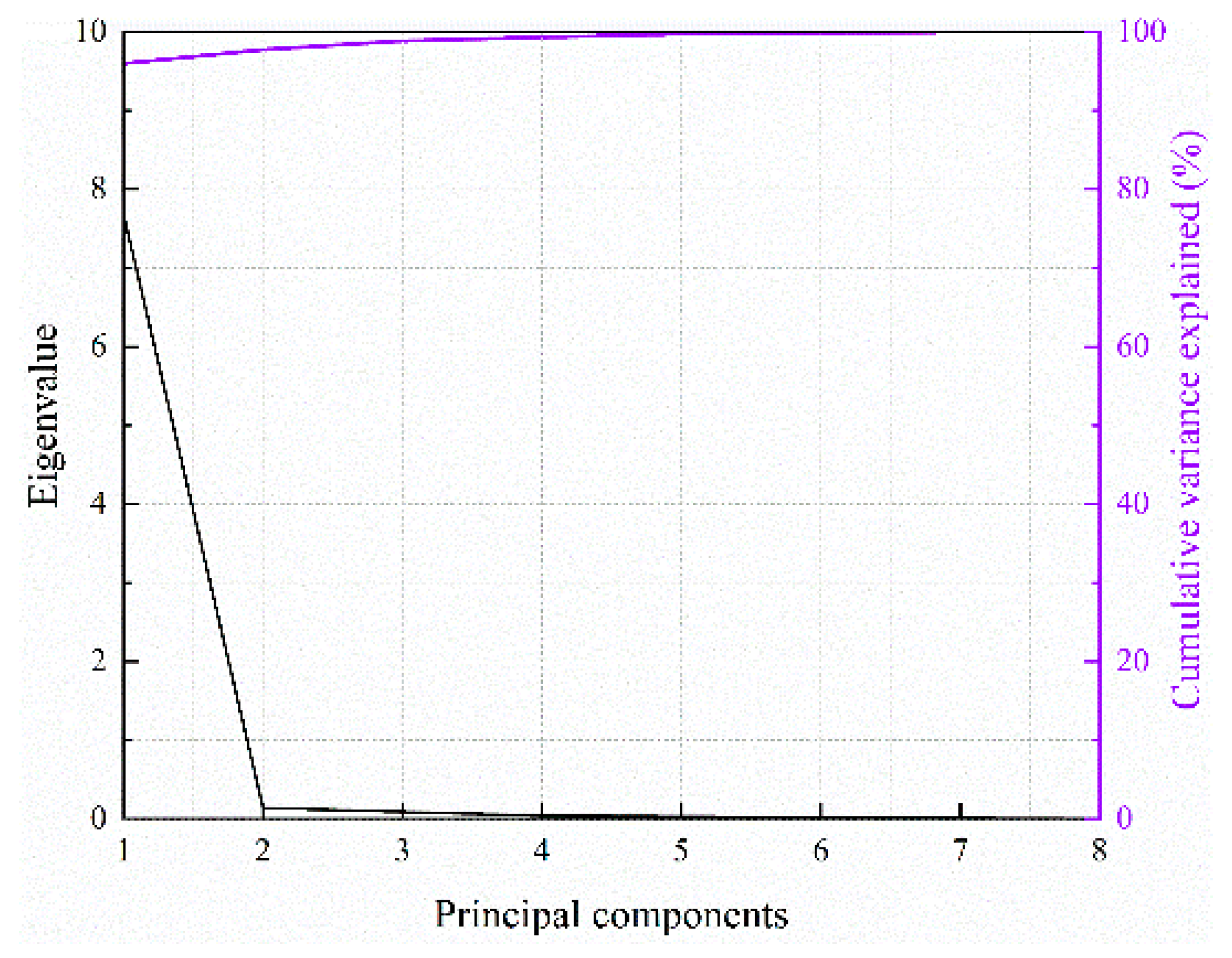
2. A Powerful Dimension-Reduction Method for PCA

The statistical analysis technique called PCA reduces a high dimension of characteristic parameters that describe the properties of a sample to a low dimension of feature parameters [31]. In most cases, the largest eigenvalue of the initial covariance matrix is associated with the information captured by the PCA. The maximum variance belongs to the first $P{C}_1$ and can explain most of the characteristic information of data variables. When the first $P{C}_1$ is not enough to explain the main characteristic information of the data variable, the second $P{C}_2$, that is, the second linear combination, is considered to explain the remaining part of the feature information, which is uncorrelated to the first $P{C}_1$. In addition, the vectors of the eigenvectors of the variance–covariance matrix are applied to specified PCs. Because all PCs are orthogonal to one another, each gathers unique information. In general, given a vector $U_1,U_2,\cdots ,U_n$ of $n$ random variables, this linear transformation permits passage from the initial space to the PC space. Meanwhile, a PC having maximum variance can be defined by the following linear transformation:

$$\mathbf{Y}=\mathbf{P}\mathbf{U}$$

(1)

$$\left[\begin{array}{ccc}{y}_1\left(x_1\right)& \cdots & y_1\left(x_n\right)\\ ⋮& \ddots & ⋮\\ y_m\left(x_1\right)& \cdots & y_m\left(x_n\right)\end{array}\right]=\left[\begin{array}{ccc}{p}_{1,T_1}& \cdots & p_{1,T_m}\\ ⋮& \ddots & ⋮\\ p_{m,T_1}& \cdots & p_{m,T_m}\end{array}\right]\left[\begin{array}{ccc}{u}_{T_1}\left(x_1\right)& \cdots & u_{T_1}\left(x_n\right)\\ ⋮& \ddots & ⋮\\ u_{T_m}\left(x_1\right)& \cdots & u_{T_m}\left(x_n\right)\end{array}\right]$$

(2)

where $\mathbf{Y}=(m\times n)$ represents the transformed variables matrix; $\mathbf{P}=(m\times m)$ indicates an orthogonal linear transformation matrix, and $\mathbf{U}=(n\times n)$ represents the examined original data matrix.

Similarly, the PCs can be converted back into their original space as follows:

$${\mathbf{P}}^{-1}\mathbf{Y}=\mathbf{U}$$

(3)

Based on Equation (3), if the matrix $\mathbf{P}=(m\times m)$ indicates an orthogonal matrix, the matrix of original data $\mathbf{U}=(n\times n)$ can be defined by:

$${\mathbf{P}}^{\mathbf{T}}\mathbf{Y}=\mathbf{U}$$

(4)

In general, the matrix of original data $\mathbf{U}=(n\times n)$ should be pre-processed and normalized before the PCA correlation matrix is analyzed to decrease the effect of the dimensions of different variables. On the other hand, since the PCs are uncorrelated, only the spatial correlation should be considered in Equation (5):

$$Y_i=\left[y_i\left(x_1\right)y_i\left(x_2\right)\cdots y_i\left(x_n\right)\right]$$

(5)

The uncorrelated nature of the PCs eliminates the necessity for cross-semivariograms and permits the independent calculation of semivariograms for each component. In the case of EDPs, this would imply that the requisite number of possible configurations may be emulated with a lesser number of PCs. The variance $Var\left(Y_i\right)$ of each PC may be estimated to determine the number of PCs that can reflect the majority of the variability in the dataset. Typically, the number of PCs that satisfy Equations (6) and (7) is used to express the features of an examined dataset.

$$Var\left[Total\right]={\displaystyle \sum _{i=1}^{m}Var\left[u_{T_i}\left(x\right)\right]}={\displaystyle \sum _{i=1}^{m}Var\left[Y_i\right]}$$

(6)

$$\%{\sigma }_{\exp l.cum}^2={\displaystyle \frac{{\displaystyle {\sum }_{i=1}^{m_{95}}Var\left[Y_i\right]}}{Var\left[Total\right]}}\ge 0.95$$

(7)

Traditionally, the first step is to perform a statistical test of the original data variables when applying PCA. For the statistical test of multivariate correlations among the examined scalar-valued IMs, Bartlett’s statistic and the Kaiser–Meyer–Olkin (KMO) statistic test are used in this study. Following the null and alternative hypotheses, the Bartlett’s statistic text can be calculated as follows:

$${\chi }^2=-\mathrm{l}\mathrm{n}\left|\mathit{R}\right|\left[(n-1)-{\displaystyle \frac{2p+5}{6}}\right]$$

(8)

where $p$ and $n$ are the number of selected scalar-valued IMs and as-recorded GMs, respectively, and $R$ indicates the correlation coefficient matrix. Under a given significance level ($\alpha =0.05$), if ${\chi }^2>{\chi }_{\alpha }^2$, the null hypothesis is generally rejected and the original variables are considered. Moreover, the KMO statistic test is utilized to determine whether the original variables are suitable for PCA by comparing the relative magnitude of the correlation coefficient and the partial correlation coefficient among the original variables. It is worth noting that the key parameters related to the input and selection of earthquake motion intensity in this paper are all implemented through MATLAB Statistics Toolbox R2018a and SPSS software 26.

3. Machine Learning

ML algorithms, which are regarded as an efficient and high-fidelity branch of application of artificial intelligence, have made continuous waves in the field of underground structures and earthquake risk assessment. The mathematical calculations of machine learning have the ability to automate analytical model building and extract effective features from massive data and also have the potential to deduce new features and mechanisms. In addition, they can improve the predictive ability of outcomes and produce reliable, repeatable decisions and results that are complementary to previous massive data with the potential to learn. ML algorithms provide a variety of classification- and regression-based approaches for structural safety assessment. It is common practice to forecast outputs that are thought of as continuous using regression-based methods. An overview of data-driven ML algorithms is given in this section.

3.1. Stepwise Regression

Stepwise (ST) regression is a multivariate statistical method that can eliminate multicollinearity among variables [32]. In the ST linear regression process, the optimal variable is automatically selected from known variables and used to establish the prediction or interpretation model of regression analysis. The ST linear regression method is designed to introduce the independent variables for which the sum of squares of the partial regression is significant in the F-test. The theoretical model is

$$\widehat{y}=a_0+{\displaystyle \sum _{i=1}^k{a}_i{x}_i}$$

(9)

where $a_0$ and $a_i$ are the constant and the coefficients of independent variables, respectively; $\widehat{y}$ indicates the predicted data of the dependent variable; $x_i$ represents a characteristic variable introduced into the regression model, which meets the requirements of the F-test statistic. It is assumed that $m-1$ variables are introduced in the regression equation and the mth variable, $x_j$, is planned to be inputted. The regression sum of squares and residuals of the equation introducing $x_j$, which contains $m$ variables, are $S{S}_r$ and $S{S}_{\sigma }$, respectively.

$$S{S}_r={\displaystyle \sum _{i=1}^n({\widehat{y}}_i-\overline{y}}{)}^2$$

(10)

$$S{S}_{\sigma }={\displaystyle \sum _{i=1}^n(y_i-{\widehat{y}}_i}{)}^2$$

(11)

where ${\widehat{y}}_i$ reflects the predicted data of the dependent variable; $y_i$ indicates the actual value; and $\overline{y}$ represents the mean of n actual values.

The partial regression sum of squares of $x_j$ is denoted by $U$, which can be written as

$$U=S{S}_r-S{S}_{r(-j)}$$

(12)

where $S{S}_{r(-j)}$ is the regression sum of squares of the equation not introducing $x_j$, which contains $m-1$ variables.

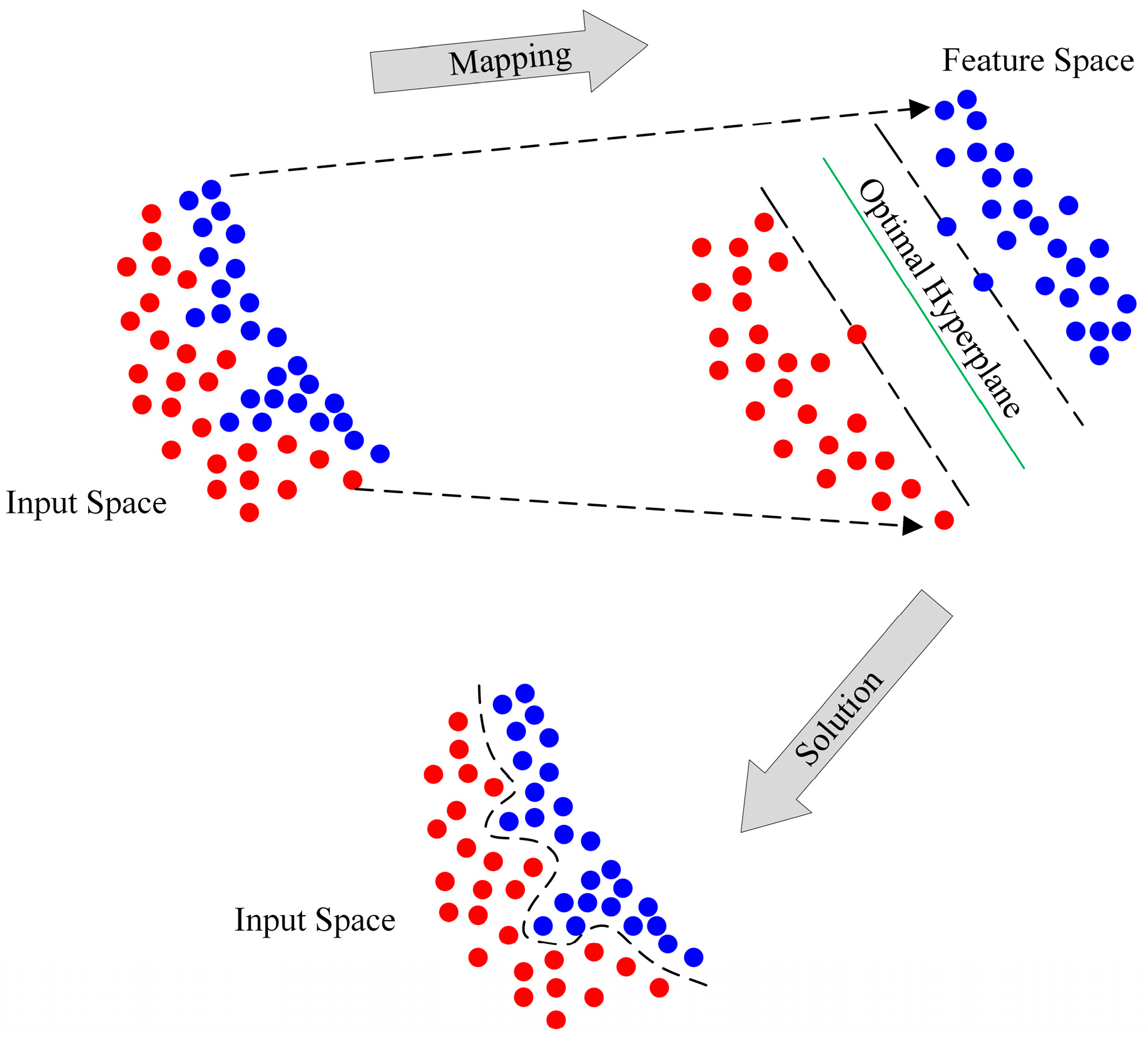
3.2. Support Vector Machine Regression

Classification and tendency analysis models are built using SVM, a supervised associated learning technique employing subsets of training data [33]. As illustrated in Figure 1, this technique divides training data into subsets based on their proximity to a hyperplane used to demarcate the border between classes. In the meantime, a non-probabilistic classifier is typically used to map the input data points from the supplied set of training data points into a higher-dimensional space in order to forecast values. Generally, a linear decision function of SVM can be written as:

$$S(x)=C^{T}x+b$$

(13)

where b indicates the bias scalar term and $C$ represents the weight vector that determines the hyperplane’s orientation.

3.3. Decision Tree Regression

A decision tree (DT) classifies or regresses data using recursive input parameter partitioning [34]. As a non-parametric classification technique, it divides the initial data into successively smaller subgroups while concurrently creating a DT, resulting in a classification or regression model with a tree fork structure. In actual use, a DT iteratively investigates the properties of the provided dataset that are most likely to predict this very same class. The outcomes of categorizing using a DT are decision nodes and leaf nodes. A leaf node represents a categorization or evaluation, but a decision node has at least two branches. The best predictor corresponds to the first or apex decision node, also known as the root node. The class of a node in the test subset may be ascertained by traversing the DT from the root node to the terminal node.

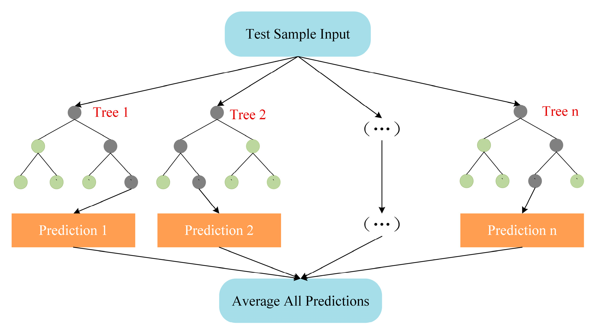
3.4. Random Forest Regression

The RF method forms a forest from several random and unrelated DTs for regression. The bootstrap resampling technique, which creates a new training sample set by repeatedly choosing k samples from the first sample set N, is crucial to this strategy, as shown in Figure 2. Then, the self-help sample set is rooted to make k DTs for the final training sample set, while the score from the DT votes determines the regression prediction for new data. The essence is an enhancement to the DT method that allows for the combination of numerous independently retrieved DTs. Every tree in the forest has the same distribution, and the correlation between them and their ability to predict regression determines the regression error.

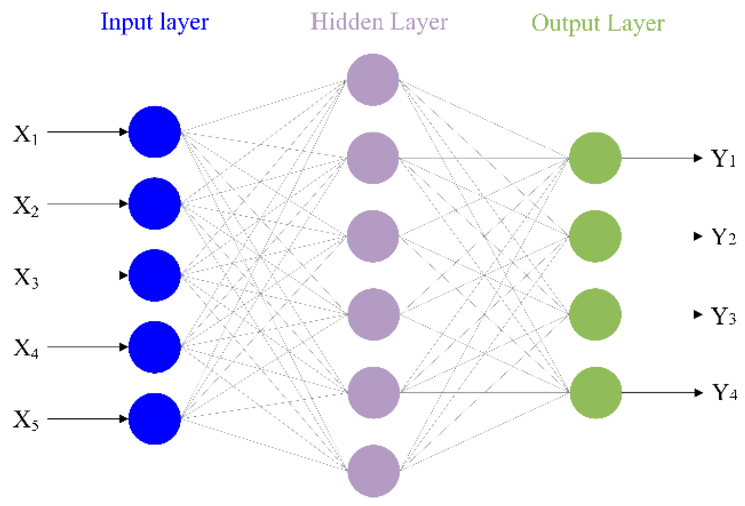
3.5. Neural Networks Regression

An NN serves as a mathematical model capturing the intricate information processing inherent in the human brain’s nervous system. It accomplishes this by approximating the understanding of biological NNs, abstracting the structure and stimulus–response mechanism of the human brain. This approach involves predicting response parameters through the establishment of nonlinear functional links among input characteristics. Illustrated in Figure 3, an NN comprises layers—input, hidden, and output—of neurons, which, in turn, represent specific activation functions. These layers form nodes or neurons, and a distinct set of weights signifies connections between each pair of neuron nodes, assigning priority to inputs for the algorithm’s learning task. Over the course of model training, these weights undergo adjustments to minimize the error between actual and anticipated values.

3.6. Gaussian Process Regression

Gaussian process (GP) regression is a non-parametric kernel statistical learning approach based on the Bayesian probability framework that is ideally suited for complicated regression issues such as high dimensionality, few samples, and nonlinearity. The model simulation requires fewer parameters compared with artificial NNs and SVM, and the optimization and convergence process is simpler to implement. Meanwhile, the hyperparameters may be acquired adaptively by locating the highest value of the log-likelihood function of the training samples, a method with flexible non-parametric inference and the probabilistic interpretation of the anticipated output. For the GP regression problem, let the dataset $D=\left\{\left(x_i,y_i\right),i=1,2,\dots ,n\right\}$ be the initial value of the model, where $x_i$ is the d-dimensional input variable and $y_i$ is the target output. According to the definition of GP regression, the mean function $f\left(x_i\right)$ obeys the multivariate Gaussian distribution can be described as:

$$f\left(x_i\right)~MVN\left[m\left(x_i\right),K\right],i=1,2,\cdots ,n$$

(14)

where $m\left(x_i\right)$ represents the mean vector of the Gaussian distribution and $K$ is the covariance matrix.

4. Framework for the Fragility Curve Fitting Method Coupling the Predicting Data

Seismic fragility analysis is a robust statistical analytical method, instrumental in assessing a structure’s seismic resilience. This assessment often involves gauging the likelihood of surpassing distinct damage states under varying earthquake intensities. Simultaneously, the vulnerability curve enhances the seismic capacity of the structure while streamlining emergency rescue plans through transparent and scientifically quantifiable means. Expressing fragility curves as lognormal cumulative distribution functions further contributes to a comprehensive understanding of a structure’s seismic performance. This approach aligns with the principles of performance-based earthquake engineering, emphasizing interconnectedness in evaluating and enhancing structural resilience [35]:

$$p_f\left(\left.EDP\ge edp\right|IM=im\right)=1-\Phi \left[{\displaystyle \frac{ln(edp)-ln({\lambda }_{EDP\left|IM\right.})}{\sqrt{{\beta }_{EDP\left|IM\right.}^2+{\beta }_C^2+{\beta }_{DS}^2}}}\right]$$

(15)

where $\Phi (\cdot )$ is the cumulative distribution function; ${\beta }_{\left.EDP\right|IM}$ represents the standard deviation; ${\beta }_c$ is the aleatory uncertainty related to the capacity of the tunnel lining and is commonly assumed to be 0.4; ${\beta }_{DS}$ is the epistemic uncertainty related to the structural DS; and ${\lambda }_{\left.EDP\right|IM}$ represents the mean value at different DSs of structures.

Generally, the traditional PSDM can be transformed as a log-linear functional form related to DM and IM samples and is expressed as:

$$ln({\lambda }_{EDP\left|IM\right.})=lna+bln(IM)+{\epsilon }_i$$

(16)

where $a$ and $b$ indicate the simple linear regression values and ${\epsilon }_i$ represents the residual error.

MLE is a technique used to derive statistical parameters from a set of structural responses characterized by a uniform distribution. This approach is instrumental in gauging the variance between the statistical trend model and the EDP within the ML-based PSDM. Employing the MLE-MSA methodology, the primary objective is to pinpoint the most probable occurrence of collapse data, stemming from a trend model rooted in statistics. The MLE-MSA technique enables the estimation of statistical parameters for the lognormal fragility function, achieved by optimizing the likelihood of observing collapse data associated with the ML-based PSDM. The MLS-MSA method can be described as [11,12,36]:

$$\widehat{\theta },\widehat{\beta }=\underset{\theta ,\beta }{{\displaystyle \arg \max }}{\displaystyle \sum _{i=1}^m\left[\mathrm{l}\mathrm{n}\left(\begin{array}{c}{N}_i\\ n_i\end{array}\right)n_i \mathrm{l}\mathrm{n}\left(\Phi \left(\frac{\mathrm{l}\mathrm{n}(x_i)-\theta }{\beta }\right)\right)+\left(N_i-n_i\right)\mathrm{l}\mathrm{n}\left(1-\Phi \left(\frac{\mathrm{l}\mathrm{n}(x_i)-\theta }{\beta }\right)\right)\right]}$$

(17)

where $\theta$ and $\beta$ are the median and the logarithmic standard deviation of the fragility function, respectively; $m$ is the number of GMs at each IM level; and $N_i$ and $n$ represents the predicted total number of structural responses and collapse number of the structural responses, respectively. Herein, the two threshold limits of the drift ratio ($\mathsf{\delta }/{2\mathrm{R}}_{\mathrm{eq}}$), namely, 0.16% and 0.18%, are obtained from dynamic analysis of CFHTs to illustrate the three damage states (DSs) of no, slight/moderate, and extensive, respectively.

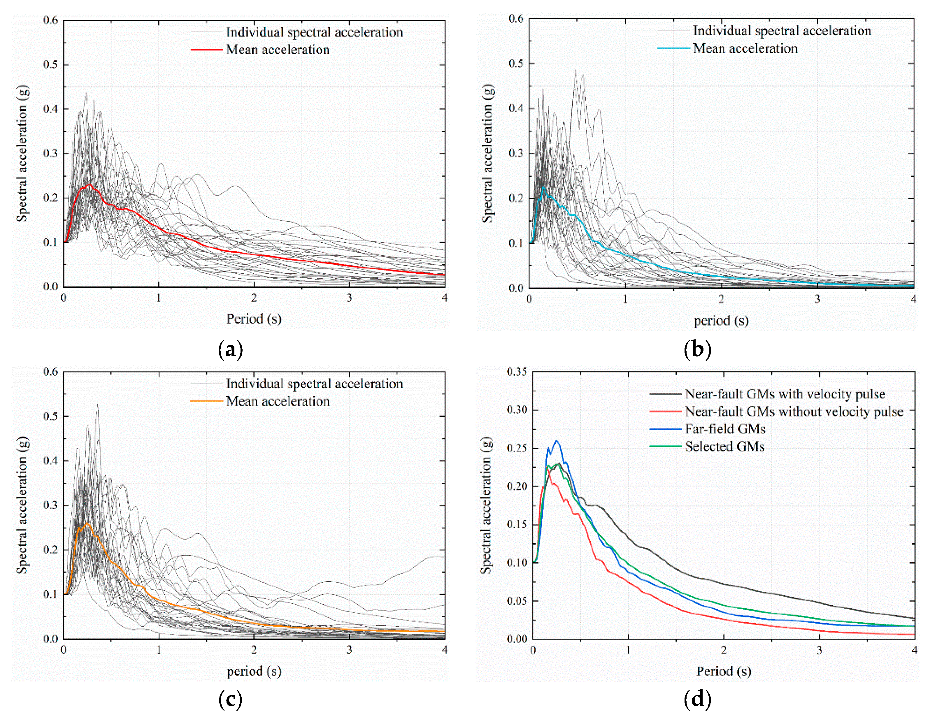
5. Pre-Processing of Ground Motions and Integrated IM

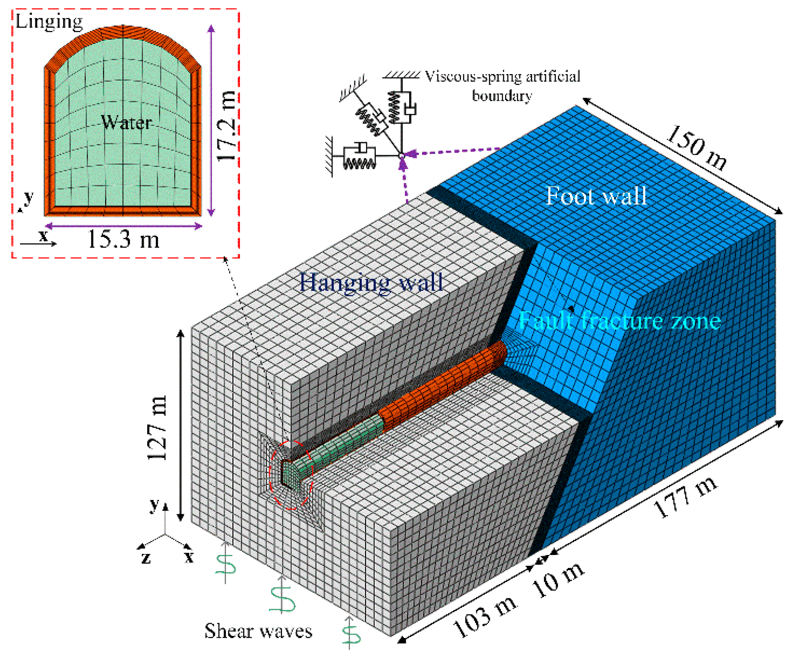
The PEER center of the United States maintains a robust database of strong ground motion (GM) records for researchers, including seismic station data, peak parameters, location, occurrence time, and fault type. Three sets of 90 as-recorded earthquakes, including near-fault GMs with velocity pulse, near-fault GMs without velocity pulse, and far-field GMs, were selected from the Strong Motion Database as the input earthquakes to obtain related data, which obey the following criteria: (i) the moment magnitude of seismic events is greater than 4.5; (ii) the PGA of the as-recorded earthquakes is more significant than 0.1 g; and (iii) the lowest usable frequency is at least 0.25 Hz or less; (iv) the as-recorded velocity pulse is unrestrained [30,37]. The spectral acceleration for single GMs under PGA = 0.1 g is plotted in Figure 4. Clearly, the spectral acceleration of different periods is significantly different for the three types of GMs. In addition, the fifteen scalar-valued intensity measurements (IMs) of the selected GMs were utilized as input variables to develop an integrated IM by the PCA method, as listed in

Table 1. Different intensity measures for the seismic fragility analysis.

Type	Description	Symbol	Definition	Unit	Reference
Amplitude	Peak ground acceleration	PGA	$PGA=\max \left|{\ddot{u}}_g(t)\right|$	g	-
	Peak ground velocity	PGV	$PGV=\max \left|{{\displaystyle \dot{u}}}_g(t)\right|$	m/s	-
	Peak ground displacement	PGD	$PGD=\max \left|u_g(t)\right|$	m	-
	Sustained maximum acceleration	SMA	The third-largest absolute peak in the acceleration time history	m/s2	[38]
	Sustained maximum velocity	SMV	The third-largest absolute peak in the velocity time history	m/s	[38]
Integral	Acceleration root-mean-Square	Arms	$a_{RMS}=\sqrt{1/t_{tot}{\int }_0^{t_{tot}}{\left[{\ddot{u}}_g(t)\right]}^{2}dt}$	g	[39]
	Velocity RMS	Vrms	$v_{RMS}=\sqrt{1/t_{tot}{\displaystyle {\int }_0^{t_{tot}}{\left[{\dot{u}}_g(t)\right]}^{2}dt}}$	m	[40]
	Displacement RMS	Drms	$d_{RMS}=\sqrt{1/t_{tot}{\displaystyle {\int }_0^{t_{tot}}{\left[u_g(t)\right]}^{2}dt}}$	m	[40]
	Arias intensity	IA	${{\displaystyle I}}_a={\displaystyle \frac{\pi }{2g}}{\displaystyle \underset{0}{\overset{t_{tot}}{\int }}{\left[{\ddot{u}}_g(t)\right]}^2}dt$	m/s	[41]
	Characteristic intensity	IC	$I_c=a_{RMS}{ }^{1.5}{t}_d{ }^{0.5}$	-	[28]
	Specific energy density	SED	$SED={\displaystyle {\int }_0^{t_{tot}}{\left[{\dot{u}}_g(t)\right]}^{2}dt}$	m2/s	[42]
	Cumulative absolute velocity	CAV	$CAV={\displaystyle \underset{0}{\overset{t_{tot}}{\int }}\left|{\ddot{u}}_g(t)\right|dt}$	m/s	[43]
Frequency content	Acceleration spectrum Intensity	ASI	$ASI={\displaystyle {\int }_{0.1}^{0.5}{S}_a(\xi =0.05,T)dT}$	m*s	[44]
	Velocity spectrum intensity	VSI	$VSI={\displaystyle {\int }_{0.1}^{0.5}{S}_v(\xi =0.05,T)dT}$	m	[44]
	Housner intensity	HI	$HI={\displaystyle {\int }_{0.1}^{0.5}PSV(\xi =0.05,T)dT}$	m	[45]

. The detailed parameters and characteristics of the data can be found in the work by Sun et al. [37].

The applicability of the selected basic scalar-valued IMs for PCA was examined according to Equations (8) and (9). Among the various combinations, the highest value of the integrated IM (PGA, PGV, PGD, ARMS, VRMS, DRMS, IC, VSI, and HI) of Bartlett’s sphericity statistic test is 26517.28, which is obviously greater than ${\chi }_{0.05}^2\left(28\right)=41.34$. In addition, the value of the KMO statistic examined among the selected scalar-valued IMs is 0.91, which means the original variables are useful. It is shown that the chosen scalar-valued IMs are appropriate for PCA by combining the findings of KMO and Bartlett’s sphericity examination. Figure 5 shows the eigenvalue and cumulative variance contribution rate of each PC by the integrated IM (PGA, PGV, PGD, ARMS, VRMS, DRMS, IC, VSI, and HI). As seen in Figure 5, the cumulative variance contribution rate of the first PC is 95.9%, whereas for the second PC, the contribution rate of 97.7% is also lower than the 99% criterion [17,18]. When the number of PCs exceeds four, the corresponding cumulative contribution rate exceeds 99%. Meanwhile, it can also be seen in Figure 5 that the trends in the fourth eigenvalues begin to stabilize. This paper extracts six PCs with a cumulative variance contribution rate of 99.9%, which can retain more information on the as-recorded GMs and establish a stronger appropriate EDP model, which is applied in the follow-up analysis.

6. Numerical Method

The current study utilized an FE model of the CFHT implemented in ABAQUS 6.14 software to carry out an incremental dynamic analysis from 0.1 g to 1.2 g. The numerical model’s detailed geometric features are presented in Figure 6, with the structure having an external width and height of 15.30 m and 17.15 m, respectively, and a lining thickness of 1.00 m. Moreover, a 60° angle and a width of 10 m for the fault are constructed between the hanging and footwall areas. Linear brick elements with 61,440 structural elements and 69,986 nodes are utilized to mesh the rock and concrete lining, while the fluid element has 3840 elements and 4941 nodes. In accordance with the transmitted wavelengths, the maximum element size is 7.0 m, which reduces the impact of the element mesh size in 3D seismic wave propagation [46]. For the linear/nonlinear mechanical property of the hanging wall and footwall, the Drucker–Prager model with mass density = 2700 kg/m³, elastic modulus = 5.0 GPa, Poisson’s ratio = 0.29, friction angle = 35°, and cohesion = 0.6 MPa is adopted to illustrate the dynamic behavior. Similarly, the Drucker–Prager model for the fault with mass density = 2000 kg/m³, elastic modulus = 0.3 GPa, Poisson’s ratio = 0.33, friction angle = 24.2°, and cohesion = 0.1 MPa is also used to describe the inelastic failure mechanism. A continuous damage–plastic concrete failure model is utilized to identify mechanical behavior and nonlinear cracking of the CFHT lining based on the combination of the theory of plasticity and the theory of damage mechanics. Material properties for the damage–plastic concrete failure model are as follows: elastic modulus = 2.8 × 10⁹ Pa, mass density = 2.45 × 10³ kg/m³, compressive yield stress = 1.67 × 10⁷ Pa, tensile yield stress = 1.78 × 10⁶ Pa, and Poisson’s ratio = 0.167. The elastoplasticity stress–strain relationships of the tunnel lining under cyclic SGM loads with different damage coefficients (0.0–1.0) are adopted to describe cumulative damage cracking according to Sidoroff’s energy equivalent method, as shown in Figure 7. In addition, the viscous-spring artificial boundary for reflecting seismic waves [47], the initial stress field [48], the nonlinear dynamic interaction among the fault fracture zone, footwall/hanging wall, and concrete lining [30], and the fluid–structure interaction are also utilized to develop the multi-physics coupling model. For brevity, in this article, the verification and detailed parameters of the model can be found in the previous work by Sun et al. [30].

7. Analysis Results and Discussion

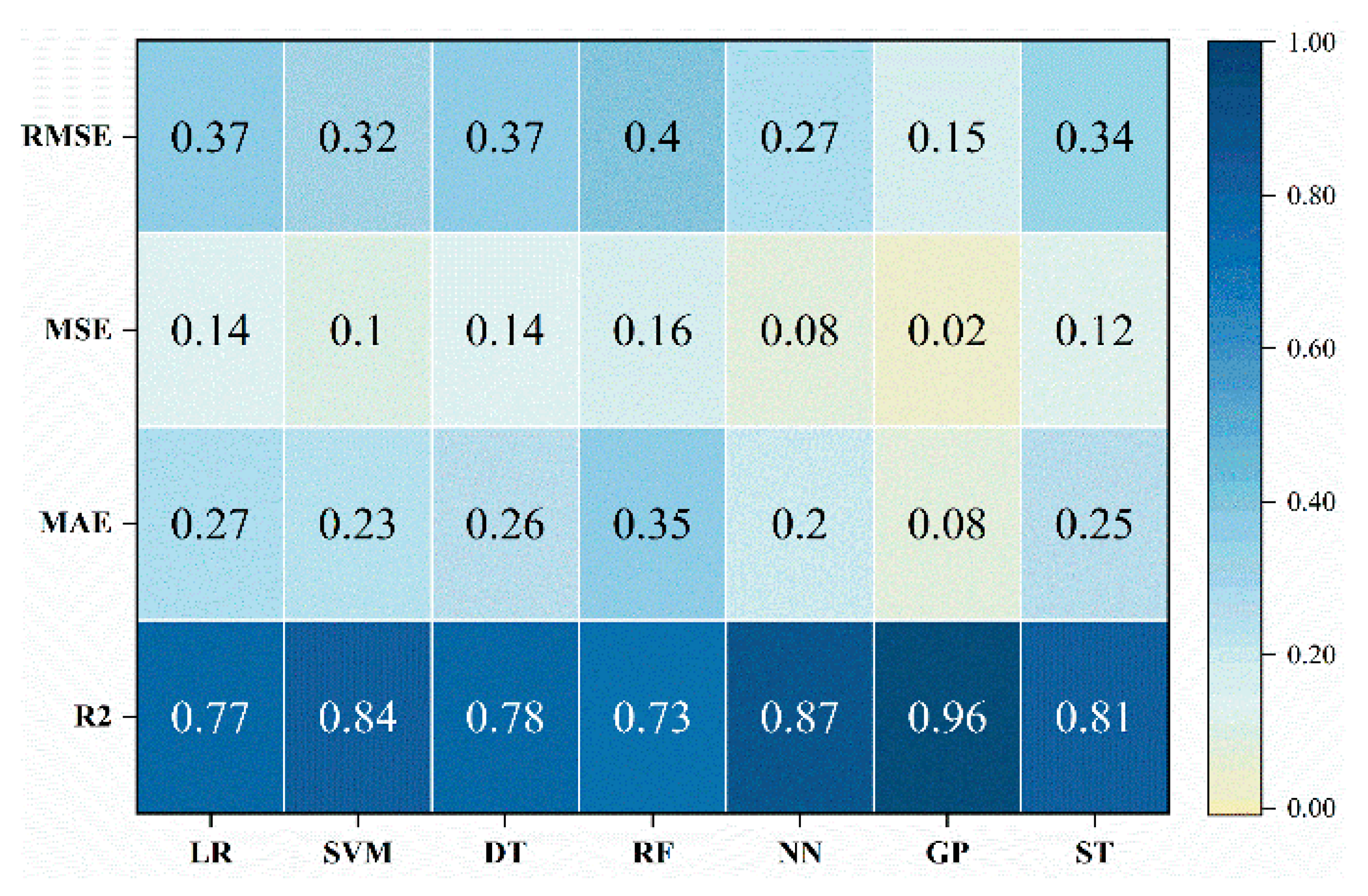
7.1. Predictive Capability Evaluation of Various ML-PCA Approaches

Initially, the predictive capability of the EDP of CFHTs based on various ML-PCA approaches was estimated to choose the optimal model for the PSDM. This study helps determine the optimal ML-PCA prediction model for the MLE-MSA approach by developing fragility curves for CFHTs. To enhance the ML-PCA model’s accuracy, the entire CFHTs EDP dataset underwent a random shuffle, resulting in two distinct subsets for training and testing. The training dataset comprises 70% of the total, while the testing dataset constitutes the remaining 30%, maintaining a proportional connection between them at a 7:3 ratio. Various regression techniques, including linear SVM, stepwise linear regression, coarse DT regression, LSboost RF regression, narrow NN regression, and quadratic rational GP regression, were employed to unveil the predictive capabilities of HTs. To evaluate predictive potential, metrics such as the coefficient of correlation (R²), root mean square error (RMSE), mean square error (MSE), and mean absolute error (MAE) were used. These metrics served as indicators of the disparity between the calculated values derived from the FE method and the predicted values.

Figure 8 shows the values of metrics for training the database of structural EDP calculated by the ML-PCA methodologies. It is observed in Figure 8 that the RMSE coefficient exhibits the lowest value in the GP regression among all the examined ML-PCA methodologies. The MSE of the next two most efficient ML-PCA methodologies is NN ($RMSE=0.33$) and SVM ($RMSE=0.32$), respectively, which are slightly greater than those of the GP regression. Moreover, the largest RMSE of 0.37 belongs to the DT methodology, which means a large difference between the predicted value and training database. Similarly, the top three strongly different ML-PCA methodologies follow the order GP < NN < SVM, compared with the other examined ML-PCA algorithms. Their corresponding MSE coefficients are 0.04, 0.09, and 0.10, respectively. Generally, the coefficients of MSE and RMSE are close to zero and the accuracy is high. On the other hand, it is found that the three ML-PCAs with the smallest MAE values are GP, NN, and SVM, with values equal to 0.11, 0.21, and 0.23, respectively. The success of the ML-PCA methodology may be seen by comparing the correlation coefficients, which show how a predicted value and EDP are related to one another. The predictive power of EDP is improved by a stronger correlation coefficient between the expected value and EDP. The correlation coefficients of the top three most efficient are GP ($R^2=0.94$) > SVM ($R^2=0.84$) > NN ($R^2=0.83$), which are slightly greater than those of ST ($\theta$). Note that the coefficients of RMSE, MSE, and MAE calculated by simple LR-PCA are significantly larger than the ML-PCA except RF. For the correlation coefficient, the value of simple LR-PCA is also larger than the ML-PCA. In other words, the simple LR-PCA.

The test dataset derived from the nonlinear dynamic analysis of the EDP of the CFHT was employed to further reveal the predictive capacity of the training models of the ML-PCA methodologies. The coefficient metrics between the test dataset and the predicted value by the trained models are compared in Figure 9. Regarding the RMSE and MSE, the coefficients of RF, LR, and DT are the top three values among the examined ML-PCA methodologies, which means that the trained models have a significant deviation in the prediction of the EDP of the CFHT under a future unknown earthquake. Simultaneously, the GP, NN, and SVM are the first low values among the examined ML-PCA methodologies. In addition, the MAE coefficients of GP, NN, and SVM, respectively, are 0.08, 0.20, and 0.23, which mean a low absolute error between the predicted values and the test database, as shown in Figure 9. In addition, Figure 9 shows that there is a close correlation among the predicted values by GP, NN, and SVM and the test database. Compared with the seven regression methodologies, the correlation coefficient of GP-PCA is greater than the six regression approaches. Considering the above-mentioned results, it is reasonable to suggest that the GP-PCA has better feasibility and reliability than the examined ML-PCA methodologies based on the RMSE, MSE, MAE, and R².

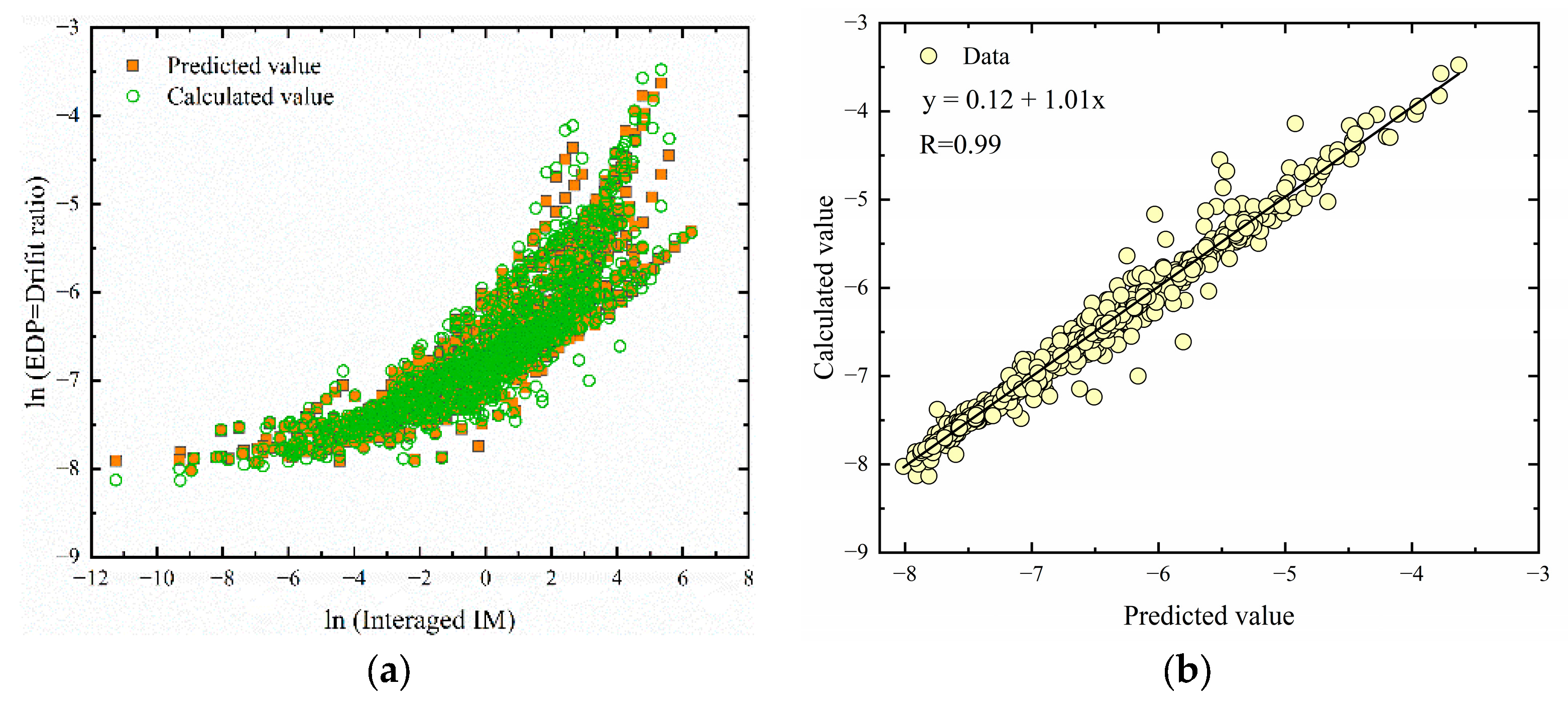
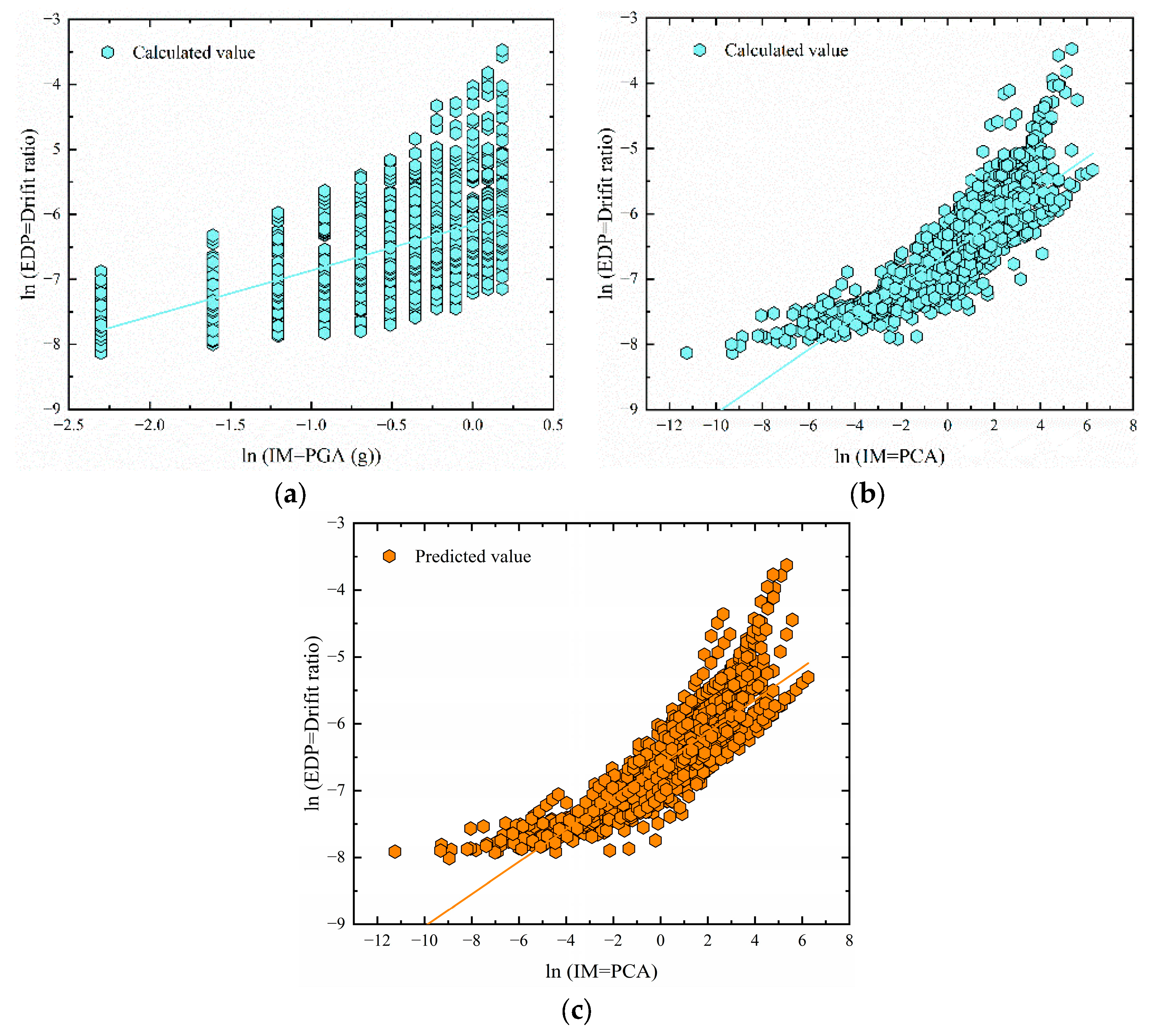
7.2. Traditional Trend Model and ML-PCA Predicted Model

The predicted value of the GP-PCA model was compared with the numerical values in the logarithmic space, as shown in Figure 10. The distribution of predicted values matches the calculated values very well over most seismic intensity ranges (Figure 10a). Also, it was discovered that there is a small discrepancy between the calculated value and the projected GP-PCA value for the CFHT EDP distribution during both low-intensity and extreme-intensity earthquakes. The GP-PCA predicted model shows a significant connection between the predicted value and the calculated value of the numerical analysis of the CFHT, as shown in Figure 10b. This suggests that the seismic assessment of the CFHT can be carried out using the projected value determined by the GP-PCA.

To investigate the discrepancy between the calculated value and predicted number by the GP-PCA mode, the traditional PSDM was utilized, further evaluating the performance of the trend models in accordance with Equation (17), as shown in Figure 11. It can be observed that the traditional PSDM related to PGA, PCA, and GP-PCA shows differences in the calculated value and the predicted value. For ease of understanding, the correlation coefficients and ${\beta }_{\mathrm{EDP}\left|IM\right.}$ are listed in

Table 2. Regression results for the calculated value and predicted value.

IMs	Probabilistic Seismic Demand Models	${\mathit{\beta }}_{\mathbf{EDP}\left|\mathit{I}\mathit{M}\right.}$	Correlation Index (R)
Peak ground acceleration (PGA)	−6.16 + 0.71ln(PGA)	0.61	0.64
Principal component analysis (PCA)	−6.61 + 0.24ln(Arms)	0.42	0.85
Gaussian process–principal component analysis (GP-PCA)	−6.61 + 0.24ln(Vrms)	0.39	0.87

, which reflect the dependency and efficiency between the IM and EDP. For the value of ${\beta }_{\mathrm{EDP}\left|IM\right.}$, the value of the traditional PSDM by PGA is slightly larger than the corresponding PSDM by PCA. This suggests that the PCA correlation index shows a very strong association (R value of 0.85) with EDP for the CFHT, suggesting that the variations in structural responses discovered through the nonlinear dynamic analysis can be partly demonstrated by the variations in PCA. Under the same conditions, the traditional PSDM of the calculated value by PCA is more dependent and efficient than the corresponding PGA, which means that the integrated IM can also improve the reliability of fragility analyses except for the ML methodology. Furthermore, the value of the correlation coefficients of PCA and GP-PCA by the traditional PSDM are almost equal. In other words, predicting values through machine learning cannot violate the mathematical statistical distribution characteristics of the EDP of the CFHTs.

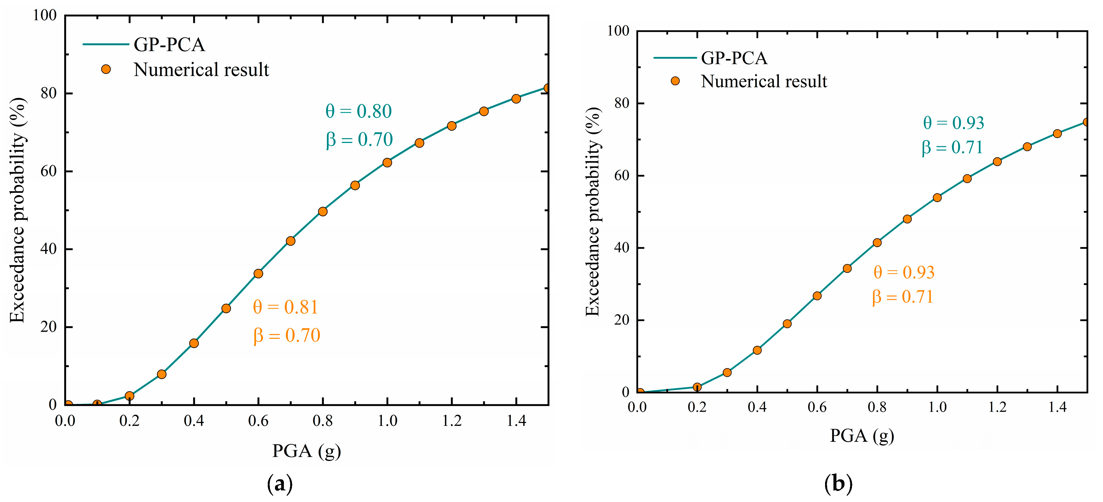
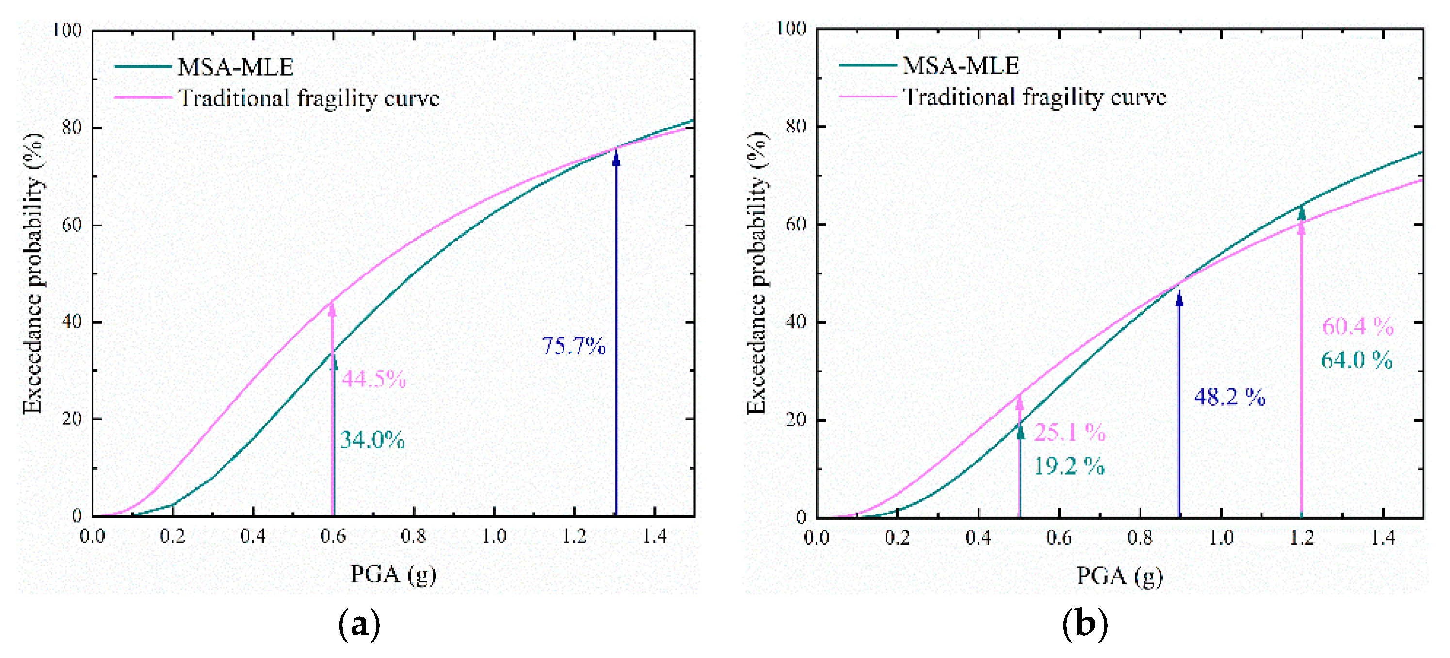
7.3. Fragility Analysis Utilizing the ML-PCA Model

According to the MSA-MLE methodology, a thorough fragility curve of the GP-PCA model for CFHTs is presented in Figure 12. It should be mentioned that in this context, the PGA is the outcropping GM that the surface seismic station saw, even if it is challenging to monitor the actual underlying GMs with accurate information. When comparing the computed fragility curves with the fragility curves based on probabilistic GP-PCA, it is important to notice that there is essentially no difference in the mean (θ) and logarithm standard deviation (β) between the GP-PCA and numerical findings. That is, the MSA-MLE method can reduce the error caused by the mathematical statistical distribution of structural EDP and the probabilistic ML-PCA model. For the second damage state, the CFHT has a probability damage of 20.0% when $\mathrm{PGA}=0.43 \mathrm{g}$, 50.0% when $\mathrm{PGA}=0.8 \mathrm{g}$, and 80.0% when $\mathrm{PGA}=1.4 \mathrm{g}$. For severe damage, the exceedance probability of the CFHT is 20.0% at $PGA=0.55$, 50.0% at $PGA=0.95 \mathrm{g}$, and 70.0% at $PGA=1.35 \mathrm{g}$, as shown in Figure 12b.

The comprehensive fragility curves based on the MSA-MLE and traditional method are compared for CFHTs (Figure 13). As shown in Figure 13, the probability of slight/moderate damage ($Drift=0.16\%$) of traditional fragility curves is equal to 44.5% at $\mathrm{PGA}=0.5 \mathrm{g}$, which approximately exceeds 30.9% compared with the exceedance probability of the MSA-MLE fragility curve. Furthermore, it can be found that only when the PGA exceeds 1.3 g, the probability of damage based on MSA-MLE is higher than the traditional method. However, the difference between the traditional fragility curve and MSA-MLE is very small. That is, the traditional method for evaluating the exceedance probability in the light/moderate damage state of CFHTs is generally higher than the MSA-MLE method. Different from the slight/moderate damage, the exceedance probability of the CFHT under extremely seismic excitation is significantly larger than the traditional method. For instance, the probability of damage to the CFHT based on MSA-MLE and the traditional method is about 64.0% and 60.4 for $\mathrm{PGA}=1.2 \mathrm{g}$, respectively. The area of the difference between the MSA-MLE and conventional methods steadily grows as the PGA rises. Conversely, the area of the difference between MSA-MLE and the traditional method gradually decreases with an increase in the PGA when the seismic intensity lies in the range of 0.0 g to 0.9 g. The above phenomenon induced by the PSDM of structures tends to underestimate or overestimate the EDP at both ends of the range of the PGA [49].

8. Final Remarks

The primary seismic performance framework in relation to earthquake intensity measures (IMs) and engineering demand factors is the fragility analysis of existing subsurface structures (EDPs). This work investigates the use of machine learning (ML) methodologies on EDP prediction and fragility curve generation to improve confidence in structural response predictions. The regression algorithms of ML are first investigated by testing to identify the optimal ML for predicting the structural response. Meanwhile, the main seismology features related to different seismic intensities are considered by the PCA, which can integrate multivariate earthquake IM features into one seismic IM feature through dimensionality reduction. The findings led to the following inferences:

(1) Compared with the seven ML-PCA methodologies in terms of the MSE, RMSE, MAE, and R² based on the training database and test database, it is found that the GP-PCA is relatively the most proper ML-PCA methodology. Accordingly, the use of GP-PCA to build the predicted model may be more efficient for predicting the EDPs among the seven ML-PCA methodologies, taken as the structural drift ratio herein. By employing training and test databases, NN-PCA and SVM-PCA showed the best performance for estimating the structure responses, closely followed by GP-PCA. Furthermore, RF-PCA is not suggested for use in predicting the structural response because of its higher MSE, RMSE, and MAE and lower R². At the same time, it is demonstrated that most ML-PCA methodologies except RF-PCA have higher predictive power for structural response than simple linear analysis.

(2) For the case study, it can be confirmed that the distribution characteristics and mathematical distribution characteristics of the predicted value by GP-PCA have a high matching degree with the calculated value. Using the conventional trend model, the case study demonstrates that integrated IM significantly affects the effectiveness, correlation, and accuracy of the PSDMs of the CFHTs. In other words, multiple seismology features can not only improve the prediction accuracy of the ML algorithm but also improve the reliability of the fragility curves of the CFHTs.

(3) The CFHT produced by MSA-MLE shows a slight difference between its GP-PCA-based fragility curves and computed value-based fragility curves, demonstrating that it is a reliable method for determining the seismic performance of CFHTs. MSA-MLE, on the other hand, overcomes the effect of assuming EDPs to be normally distributed and can also be integrated with statistical parameters of ML algorithms, making it the most appropriate method for fragility analysis of CFHTs. Additionally, there are still some limitations, such as combining the various seismology characteristics of ground motions, using a variety of evaluation indicators of the structural response, taking into account the complex engineering environment and the geometrical properties of HTs, and using various seismic input mechanisms and probabilistic seismic hazard analysis for further research. In addition, the hyper-parameter of the machine learning method also be deeply studied.

It is known that different formation parameter distributions and terrain characteristics will be encountered in actual water conservancy projects. Therefore, the hydraulic tunnel studied in this paper is suitable for actual projects with relatively large fault fracture zones. In addition, this complex prediction framework can be applied by developing a practical engineering monitoring system that is compatible with frequent earthquakes in future work.

References

1. Hashash, Y.M.A.; Hook, J.J.; Schmidt, B.; Yao, J.I.C. Seismic design and analysis of underground structures. Tunn. Undergr. Sp. Technol. 2001, 16, 247–293. [Google Scholar] [CrossRef]
2. Li, T. Damage to mountain tunnels related to the Wenchuan earthquake and some suggestions for aseismic tunnel construction. Bull. Eng. Geol. Environ. 2012, 71, 297–308. [Google Scholar] [CrossRef]
3. Shen, Y.; Gao, B.; Yang, X.; Tao, S. Seismic damage mechanism and dynamic deformation characteristic analysis of mountain tunnel after Wenchuan earthquake. Eng. Geol. 2014, 180, 85–98. [Google Scholar] [CrossRef]
4. Wang, X.; Chen, J.; Xiao, M. Seismic damage assessment and mechanism analysis of underground powerhouse of the Yingxiuwan Hydropower Station under the Wenchuan earthquake. Soil Dyn. Earthq. Eng. 2018, 113, 112–123. [Google Scholar] [CrossRef]
5. Wang, Z.Z.; Zhang, Z. Seismic damage classification and risk assessment of mountain tunnels with a validation for the 2008 Wenchuan earthquake. Soil Dyn. Earthq. Eng. 2013, 45, 45–55. [Google Scholar] [CrossRef]
6. Yu, H.; Chen, J.; Bobet, A.; Yuan, Y. Damage observation and assessment of the Longxi tunnel during the Wenchuan earthquake. Tunn. Undergr. Sp. Technol. 2016, 54, 102–116. [Google Scholar] [CrossRef]
7. Baker, J.W. Quantitative classification of near-fault ground motions using wavelet analysis. Bull. Seismol. Soc. Am. 2007, 97, 1486–1501. [Google Scholar] [CrossRef]
8. Bazzurro, P.; Cornell, C.A.; Shome, N.; Carballo, J.E. Three proposals for characterizing MDOF nonlinear seismic response. J. Struct. Eng. 1998, 124, 1281–1289. [Google Scholar] [CrossRef]
9. Cornell, C.A.; Jalayer, F.; Hamburger, R.O.; Foutch, D.A. Probabilistic basis for 2000 SAC federal emergency management agency steel moment frame guidelines. J. Struct. Eng. 2002, 128, 526–533. [Google Scholar] [CrossRef]
10. Baker, J.W. Efficient analytical fragility function fitting using dynamic structural analysis. Earthq. Spectra 2015, 31, 579–599. [Google Scholar] [CrossRef]
11. Kim, T.; Song, J.; Kwon, O.-S. Probabilistic evaluation of seismic responses using deep learning method. Struct. Saf. 2020, 84, 101913. [Google Scholar] [CrossRef]
12. Kiani, J.; Camp, C.; Pezeshk, S. On the application of machine learning techniques to derive seismic fragility curves. Comput. Struct. 2019, 218, 108–122. [Google Scholar] [CrossRef]
13. Qin, S.; Cheng, Y.; Zhou, W.H. State-of-the-art review on pressure infiltration behavior of bentonite slurry into saturated sand for TBM tunneling. Smart Constr. Sustain. Cities 2023, 1, 14. [Google Scholar] [CrossRef]
14. Huang, H.; Sun, Q.; Xu, T.; Zhou, W. Mechanism analysis of foam penetration in EPB shield tunnelling with a focus on FER and soil particle size. Undergr. Space 2024, 17, 170–187. [Google Scholar] [CrossRef]
15. Sun, B.; Wang, P.X.; Deng, M.; Fang, H.; Xu, J.; Zhang, S.; Wang, C. Seismic performance assessment of hydraulic tunnels considering oblique incoming nonstationary stochastic SV waves based on the generalized PDEM. Tunn. Undergr. Space Technol. 2024, 143, 105481. [Google Scholar] [CrossRef]
16. Sun, B.; Deng, M.; Zhang, S.; Liu, W.; Xu, J.; Wang, C.; Cui, W. Efficient Fragility Analysis of Cross-Fault Hydraulic Tunnels Combining Support Vector Machine and Improved Cloud Method. J. Earthq. Eng. 2024, 28, 2403–2421. [Google Scholar] [CrossRef]
17. Jeddi, A.B.; Shafieezadeh, A.; Hur, J.; Ha, J.; Hahm, D.; Kim, M. Multi-hazard typhoon and earthquake collapse fragility models for transmission towers: An active learning reliability approach using gradient boosting classifiers. Earthq. Eng. Struct. Dyn. 2022, 51, 3552–3573. [Google Scholar] [CrossRef]
18. Liu, C.; Macedo, J. Machine learning-based models for estimating seismically-induced slope displacements in subduction earthquake zones. Soil Dyn. Earthq. Eng. 2022, 160, 107323. [Google Scholar] [CrossRef]
19. Huang, H.; Burton, H.V. Dynamic seismic damage assessment of distributed infrastructure systems using graph neural networks and semi-supervised machine learning. Adv. Eng. Softw. 2022, 168, 103113. [Google Scholar] [CrossRef]
20. Kourehpaz, P.; Molina Hutt, C. Machine Learning for Enhanced Regional Seismic Risk Assessments. J. Struct. Eng. 2022, 148, 4022126. [Google Scholar] [CrossRef]
21. Yu, X.; Wang, M.; Ning, C. A machine-learning-based two-step method for failure mode classification of reinforced concrete columns. J. Build. Struct. 2022, 43, 220. [Google Scholar]
22. Morgenroth, J.; Khan, U.T.; Perras, M.A. An overview of opportunities for machine learning methods in underground rock engineering design. Geosciences 2019, 9, 504. [Google Scholar] [CrossRef]
23. Chimunhu, P.; Topal, E.; Ajak, A.D.; Asad, W. A review of machine learning applications for underground mine planning and scheduling. Resour. Policy 2022, 77, 102693. [Google Scholar] [CrossRef]
24. Mahmoodzadeh, A.; Mohammadi, M.; Ibrahim, H.H.; Noori, K.M.G.; Abdulhamid, S.N.; Ali, H.F.H. Forecasting sidewall displacement of underground caverns using machine learning techniques. Autom. Constr. 2021, 123, 103530. [Google Scholar] [CrossRef]
25. Pu, Y.; Apel, D.B.; Hall, R. Using machine learning approach for microseismic events recognition in underground excavations: Comparison of ten frequently-used models. Eng. Geol. 2020, 268, 105519. [Google Scholar] [CrossRef]
26. Hu, Z.; Wei, B.; Jiang, L.; Li, S.; Yu, Y.; Xiao, C. Assessment of optimal ground motion intensity measure for high-speed railway girder bridge (HRGB) based on spectral acceleration. Eng. Struct. 2022, 252, 113728. [Google Scholar] [CrossRef]
27. Padgett, J.E.; Nielson, B.G.; DesRoches, R. Selection of optimal intensity measures in probabilistic seismic demand models of highway bridge portfolios. Earthq. Eng. Struct. Dyn. 2008, 37, 711–725. [Google Scholar] [CrossRef]
28. Park, Y.-J.; Ang, A.H.-S.; Wen, Y.K. Seismic damage analysis of reinforced concrete buildings. J. Struct. Eng. 1985, 111, 740–757. [Google Scholar]
29. Yan, Y.; Xia, Y.; Yang, J.; Sun, L. Optimal selection of scalar and vector-valued seismic intensity measures based on Gaussian Process Regression. Soil Dyn. Earthq. Eng. 2022, 152, 106961. [Google Scholar] [CrossRef]
30. Sun, B.; Liu, W.; Deng, M.; Zhang, S.; Wang, C.; Guo, J.; Wang, J.; Wang, J. Compound intensity measures for improved seismic performance assessment in cross-fault hydraulic tunnels using partial least-squares methodology. Tunn. Undergr. Sp. Technol. 2023, 132, 104890. [Google Scholar]
31. Abdi, H.; Williams, L.J. Principal component analysis. Wiley Interdiscip. Rev. Comput. Stat. 2010, 2, 433–459. [Google Scholar]
32. Thompson, B. Stepwise regression and stepwise discriminant analysis need not apply here: A guidelines editorial. Educ. Psychol. Meas. 1995, 55, 525–534. [Google Scholar] [CrossRef]
33. Boser, B.E.; Guyon, I.M.; Vapnik, V.N. A training algorithm for optimal margin classifiers. In Proceedings of the Fifth Annual Workshop on Computational Learning Theory, Pittsburgh, PA, USA, 27–29 July 1992; pp. 144–152. [Google Scholar]
34. Myles, A.J.; Feudale, R.N.; Liu, Y.; Woody, N.A.; Brown, S.D. An introduction to decision tree modeling. J. Chemom. A J. Chemom. Soc. 2004, 18, 275–285. [Google Scholar] [CrossRef]
35. Ellingwood, B. Validation studies of seismic PRAs. Nucl. Eng. Des. 1990, 123, 189–196. [Google Scholar] [CrossRef]
36. Baker, J.W. Probabilistic structural response assessment using vector-valued intensity measures. Earthq. Eng. Struct. Dyn. 2007, 36, 1861–1883. [Google Scholar] [CrossRef]
37. Sun, B.; Deng, M.; Zhang, S.; Wang, C.; Cui, W.; Li, Q.; Xu, J.; Zhao, X.; Yan, H. Optimal selection of scalar and vector-valued intensity measures for improved fragility analysis in cross-fault hydraulic tunnels. Tunn. Undergr. Sp. Technol. 2023, 132, 104857. [Google Scholar] [CrossRef]
38. Nuttli, O.W. The Relation of Sustained Maximum Ground Acceleration and Velocity to Earthquake Intensity and Magnitude; US Army Engineer Waterways Experiment Station: Vicksburg, MS, USA, 1979. [Google Scholar]
39. Dobry, R.; Idriss, I.M.; Ng, E. Duration characteristics of horizontal components of strong-motion earthquake records. Bull. Seismol. Soc. Am. 1978, 68, 1487–1520. [Google Scholar]
40. Kramer, S.L. Geotechnical earthquake engineering. Bull. Earthq. Eng. 2013, 12, 1049–1070. [Google Scholar] [CrossRef]
41. Arias, A. Measure of Earthquake Intensity; Massachusetts Institute of Technology: Cambridge, MA, USA; University of Chile: Santiago, Chile, 1970. [Google Scholar]
42. Bolt, B.A. Duration of strong ground motion. In Proceedings of the 5th World Conference on Earthquake Engineering, Rome, Italy, 25–29 June 1973; pp. 1304–1313. [Google Scholar]
43. Reed, J.W.; Kassawara, R.P. A criterion for determining exceedance of the operating basis earthquake. Nucl. Eng. Des. 1990, 123, 387–396. [Google Scholar] [CrossRef]
44. Von Thun, J.L. Earthquake ground motions for design and analysis of dams Earthq. Eng. soil Dyn. II-recent Adv. Ground-Motion Eval. 1988, 20, 463–481. Available online: https://api.semanticscholar.org/CorpusID:132807569 (accessed on 30 July 2024).
45. Housner, G.W. Spectrum Intensities of Strong-Motion Earthquakes; Earthquake Engineering Research Institute: Oakland, CA, USA, 1952. [Google Scholar]
46. Kuhlemeyer, R.L.; Lysmer, J. Finite element method accuracy for wave propagation problems. J. Soil Mech. Found. Div. 1973, 99, 421–427. [Google Scholar] [CrossRef]
47. Liu, J.B.; Du, Y.X.; Du, X. 3D viscous-spring artificial boundary in time domain. Earthq. Eng. Eng. Vib. 2006, 5, 93–102. [Google Scholar] [CrossRef]
48. Wang, Z.; Pedroni, N.; Zentner, I.; Zio, E. Seismic fragility analysis with artificial neural networks: Application to nuclear power plant equipment. Eng. Struct. 2018, 162, 213–225. [Google Scholar] [CrossRef]
49. Huang, P.; Chen, Z. Fragility analysis for subway station using artificial neural network. J. Earthq. Eng. 2021, 26, 6724–6744. [Google Scholar] [CrossRef]
Figure 1. The fundamental concept of SVM.
Buildings 14 02608 g001
Figure 2. The fundamental concept of RF.
Buildings 14 02608 g002
Figure 3. The fundamental concept of an NN.
Buildings 14 02608 g003
Figure 4. Spectral acceleration for the selected GMs [30,37]: (a) near-fault GMs with velocity pulse, (b) near-fault GMs without velocity pulse, (c) far-field GMs, and (d) the 90 selected GMs.
Buildings 14 02608 g004
Figure 5. Eigenvalue and cumulative variance contribution rate to the PCs.
Buildings 14 02608 g005
Figure 6. Information on the 3D computational FE model.
Buildings 14 02608 g006
Figure 7. Stress–strain curve of the concrete lining. (a) Damage factor and compressive stress–strain. (b) Damage factor and tensile stress–strain.
Buildings 14 02608 g007
Figure 8. The statistical coefficients of the RMSE, MSE, MAE, and R2.
Buildings 14 02608 g008
Figure 9. The statistical coefficients of the RMSE, MSE, MAE, and R2.
Buildings 14 02608 g009
Figure 10. Comparison of the calculated value and predicted value by GP-PCA. (a) Distribution. (b) Correlation.
Buildings 14 02608 g010
Figure 11. Traditional probabilistic seismic demand analysis for the calculated value and predicted value. (a) PGA. (b) PCA. (c) GP-PCA.
Buildings 14 02608 g011
Figure 12. Comparison of the exceedance probability of the CFHT. (a) Slight/moderate damage. (b) Severe damage.
Buildings 14 02608 g012
Figure 13. Comparison of the exceedance probability between the MSA-MLE and traditional fragility curves. (a) Slight/moderate damage. (b) Severe damage.
Buildings 14 02608 g013