Article

A Simple Explicit Formula for Evaluating the Total Capacity of Chilled-Water Cooling Coils under Wet Conditions

1
School of Environment and Energy Engineering, Beijing University of Civil Engineering and Architecture, Beijing 100044, China
2
Division of Urban Construction, Beijing University of Technology, Beijing 100124, China
*
Author to whom correspondence should be addressed.
Buildings 2024, 14(9), 2630; https://doi.org/10.3390/buildings14092630
Submission received: 11 July 2024 / Revised: 19 August 2024 / Accepted: 21 August 2024 / Published: 24 August 2024
(This article belongs to the Section Building Energy, Physics, Environment, and Systems)

Abstract

:
A simple explicit formula for evaluating the total capacity of chilled-water cooling coils under wet conditions is reported in this paper. The formula is developed through theoretical and analogical analysis from a practical viewpoint. With the formula, a wet coil’s total cooling capacity can be predicted straightforwardly, given the inlet air and water conditions. The formula was cross-validated against a set of catalog performance data from a series of fan coil unit (FCU) coils and simulated performance data from a series of air handling unit (AHU) coils. The mean errors in the calculated results of the present formula did not exceed 5% in the training and test sets for each coil, showing it has good accuracy and generalizability over a wide operating range and various coil types. This formula is expected to have wide applications in energy simulation and control optimization of building air-conditioning systems.

1. Introduction

Chilled-water cooling coils are widely used in building air-conditioning systems for air cooling and dehumidifying. As a main component of air handling units (AHU) or fan coil units (FCU), it interconnects the chilled water loop to the air loop, and it transfers the cooling energy by forcing air flow over the coil and into the conditioned space. In practice, cooling coils are operated under various conditions (e.g., varying air or water flows, varying inlet air temperature and humidity, or varying inlet water temperature). They often operate under wet conditions where the passing moist air drops below its dewpoint and moisture condensates [1,2,3].
The total capacity of a chilled-water cooling coil is a key parameter for its energy performance, and it is significantly influenced by varying operation conditions [4]. Because of the dominant role of wet conditions in real operation and the complexity of the coupled heat and mass transfer in the dehumidification process, evaluating the cooling coil’s total capacity under wet conditions is important in the energy simulation and operation optimization of building air-conditioning systems.
There is a rich literature on modeling cooling and dehumidifying coils for different purposes and different available performance data resources [1,2,3,4,5,6,7,8,9,10,11,12,13,14,15]. Traditionally, the cooling coil models can be classified into two schemes: (1) multi-node numerical scheme and (2) lumped scheme.
The multi-node numerical scheme is commonly used in computational fluid dynamics and heat transfer. In a multi-node scheme, the cooling coil is discretized into numerous segments along the water and air flow paths. Governing equations and correlations for heat and mass transfer are established in each segment. Each segment’s heat exchange is calculated sequentially from the water and air inlets to the outlets and iteratively until convergence is met. This numerical method can analyze complex circuiting arrangements and consider the local variations of parameters along the coil, but it requires coil geometry details and consumes a long computation time. It is adopted by [3,4,5,6,16,17,18,19,20,21,22,23,24,25,26] and is mainly used for design optimization and dynamic control of cooling coils.
The lumped scheme is considered the easiest approach to simplify the performance calculation of cooling coils with reasonable accuracy and less computation time. The inlet and outlet conditions and their psychrometric process for the lumped scheme are illustrated in Figure 1. In a lumped scheme, local variations of parameters on air and water sides are neglected, mathematical relations between the inlet and outlet conditions are derived, and the calculation is made for the entire coil to seek the solution of unknown variables, including the total cooling capacity. The mathematical relations for the entire coil are generally obtained by four approaches: entirely empirical correlations [12,22]; analytical approach [27,28]; LMTD (log mean temperature difference) or LMED (log mean enthalpy difference) approach [1,8,29,30]; and, ε-NTU approach [31,32,33,34,35,36,37,38,39,40,41,42]. These approaches in the literature differ regarding model assumptions, heat transfer correlations, whether coil geometry information is required, and whether iterative calculations are required.
The ε-NTU-based lumped models of cooling and dehumidifying coils are primarily applied in the energy simulation and control optimization of building air-conditioning systems. Among the mentioned four lumped approaches, the advantages of the ε-NTU methods are: (1) they have more physical basis and physical meaning than the entirely empirical correlations; (2) they require fewer or no coil geometry data, which is hard to obtain, compared with the analytical methods; (3) they require fewer iterations for coil performance calculation than the LMTD or LMED methods [43]. Thus, they have been widely adopted in popular building energy simulation toolkits like DeST (Ver. 20230713), EnergyPlus (Ver. 24.1.0), and TRNSYS (Ver. 18.02) [39,40,41]. DeST uses a temperature-based ε-NTU method [43,44], while EnergyPlus and TRNSYS use an enthalpy-based ε-NTU method [38]. The key equations and variables used for the enthalpy- and temperature-based ε-NTU methods are summarized in Table 1. Note that (1) there are two effectiveness relations used in the classical ε-NTU-based model for a wet cooling coil, aiming at the entire coil and the air side, respectively; (2) the counterflow configuration is taken as an example for the overall effectiveness of the coil and it is similar for a crossflow configuration or others by replacing the overall effectiveness relation. Readers can refer to the literature [38,43,44] for more details.
However, from the perspective of total cooling capacity calculation, most of the existing lumped models, including the ε-NTU methods, have some common drawbacks: they involve multiple equations that may be complex and difficult to replicate, and they need a simultaneous and iterative solution procedure since the equations usually contain a few “lumped” parameters that depend on both inlet and outlet conditions and may be unknown at the beginning of the calculation. Such parameters for the entire coil process are, for example, the sensible heat ratio Q s / Q in the analytical solution proposed by Xia et al. [28], the fictitious specific heat c s , or moisture separation coefficient ξ in the effectiveness models listed in Table 1.
There are several ways to avoid the iteration in traditional ε-NTU solutions. A strategy to avoid iteration is to approximate such parameters by the inlet conditions only, as adopted by Lee’s explicit model [30] and some simple cooling coil models in EnergyPlus and TRNSYS [40,41]. However, this strategy for a lumped model may not be appropriate and cause large errors since the inlet and outlet conditions of cooling and dehumidifying coils may differ significantly. The appropriate value of a lumped parameter is an average value evaluated by both inlet and outlet conditions rather than that approximated by inlet conditions only [38].
Another way to overcome the above issues of lumped models is to find an explicit formula for calculating the total cooling capacity of wet cooling coils. Wang et al. [7] proposed a practical single-formula model in 2004, which expressed the total cooling capacity of a wet coil as a function of the air inlet wet bulb temperature, water inlet temperature, air flow rate, and water flow rate and had two or three constants to be determined. The formula can directly evaluate the total cooling capacity of a cooling coil given the inlet conditions without any iterative calculation and any coil geometry information. It is simple and was reported to be accurate by [7,45]. However, it assumed a fixed temperature difference along the coil and used an identical exponent value for air and water flows, which was unusual in heat transfer correlations, and it was only tested with very limited coil types and in very limited conditions.
The paper aims to propose a novel, simple, yet accurate formula for evaluating the total cooling capacity of chilled-water cooling coils under wet conditions. The scientific novelty of the formula includes that (1) it is based on theoretical and analogical analysis, (2) it does not need any iterative calculation nor any coil geometric information like other lumped models do, and (3) it has been cross-validated with a large set of FCU and AHU coil performance data. The formula is based on an enthalpy difference instead of a temperature difference. It contains five unknown constants, which use two separate exponents for air and water flows in the correlation and can be determined through a small number of coil performance data. In the following sections, we will introduce the development of the formula, give the procedure for determining the unknown constants, and cross-validate the formula with a large set of coil performance data, including the catalog performance data of a series of FCU coils and simulated performance data of a series of AHU coils via a known ε-NTU method.

2. Proposed Calculation Formula

2.1. Mathematical Formulation

In the following, we first introduce the general integral expression of the total cooling capacity of a wet cooling coil based on heat transfer principles. Then, we use an analogy method to establish the final formula to calculate the total cooling capacity explicitly.
The schematic of a chilled-water cooling coil is shown in Figure 1. The inlet and outlet variables are listed in Table 1. In evaluating its thermal performance, a chilled-water coil can be normally treated as a water/air heat exchanger. A condensate film is on the coil’s surface for wet conditions, as shown in Figure 2a. For simplifying the coupled heat and mass transfer process, the following assumptions are usually made:
(1)
The energy flow due to the condensate draining from the coil is small compared to the other energy terms and is neglected.
(2)
The coil surface is assumed to be totally and evenly wet. It has been proven that the error caused by approximating a partially wet coil as totally wet is generally less than 5% [2].
(3)
The temperature gradients along the thickness of the coil surface and condensate film are neglected since they are thin. Thus, the surface and the film have an identical temperature.
With the assumptions, the fundamental governing equations for energy flows taking place in a control volume of the wet coil, as shown in Figure 2b, can be established as follows:
On the air side, the energy transfer d Q at the control volume is given by:
d Q = m a d h a
Meanwhile, it equals the energy transfer between the coil surface and the air stream, which is driven by the enthalpy difference between the enthalpy of saturated air at the coil surface temperature ( h s , s a t ) and the enthalpy of the air stream far from the surface ( h a ), and can be represented by [38]:
d Q = η o U a c a h a h s , s a t d A a
On the water side, the energy transfer is given by:
d Q = m w c w d t w
d Q = U w t s t w d A w
Define an effective specific heat, c s , as the change in enthalpy to temperature along the moist air saturation line and assume it is constant for the entire coil. It is represented by:
c s = d h w , s a t d t w t w = h s , s a t h w , s a t t s t w
The heat transfer area on the air side ( d A a ) and that on the water side ( d A w ) for the control volume follows Equation (6).
d A a d A w = A a A w
Substituting Equations (5) and (6), Equations (3) and (4) can be rewritten as:
d Q = m w c w c s d h w , s a t
d Q = U w c s h s , s a t h w , s a t d A w = U w A w c s A a h s , s a t h w , s a t d A a
The energy transfer at a unitary area and the total area of the wet coil can be represented by Equation (9) and Equation (11), respectively.
d Q d A a = h a h s , s a t c a η o U a = h s , s a t h w , s a t c s A a U w A w = h a h w , s a t c a η o U a + c s A a U w A w = h a h w , s a t A a c a η o U a A a + c s U w A w = U A h A a h a h w , s a t
U A h = c a η o U a A a + c s U w A w 1
Q = 0 A a d Q = 0 A a U A h A a h a h w , s a t d A a = U A h A a 0 A a h a h w , s a t d A a
Equation (11) gives an integral form for evaluating the total cooling capacity of the wet coil. It shows that the total cooling capacity of the coil is a product of the enthalpy-based overall heat exchange coefficient at a unitary area and the integral of the enthalpy difference between the passing air and the saturated air at the chilled water temperature ( h a h w , s a t ) along the coil surface. The enthalpy difference varies along the coil surface, and the variation cannot be neglected. It can be proven that solving the integral in Equation (11) will further derive an LMED solution in Equation (12) or an ε-NTU solution in Equation (13) [38,44].
Q = U A h Δ h L M
Q = m a ε h a , i h w , s a t , i
Equation (11) can help theoretically explain why the iterative calculation was usually required in traditional LMED and ε-NTU solutions since the equations contain a few parameters that depend on both inlet and outlet conditions and may be unknown at the beginning of the calculation. It also indicates that the existing explicit methods [7,26,40,41], which can avoid iterations and rely on additional heat transfer assumptions, may be rough and lead to a loss of accuracy, as mentioned in the introduction section.
To avoid the drawbacks of traditional LMED and ε-NTU solutions and keep the rigor of derivation, we use an analogy method instead to establish the explicit expression of Q .
We first define a new effective energy transfer coefficient, S E , to replace the product of effectiveness and air flow rate ( m a ε ) in Equation (13). Thus, the total heat transfer rate of the wet coil is expressed by:
Q = S E h a , i h w , s a t , i
where S E is the cooling capacity of the wet coil provided by the action of unit inlet air-water enthalpy difference in   W   kg / J . Since S E = Q / ( h a , i h w , s a t , i ) = m a ε , S E is also a form of heat transfer efficiency, which can be used as an index to evaluate the heat and moisture exchange perfection of cooling coils under wet conditions. For a cooling coil with a fixed structure, the coefficient S E could be only related to the flow states and inlet condition on the air and water sides.
From a physical viewpoint, the definition of S E for a wet coil is similar to the definition of the overall heat transfer efficiency S w u used in the thermal performance calculation of a spray chamber in literature [44] and the overall heat transfer coefficient U A in the temperature-based ε-NTU methods [43,44]. In engineering practice, S w u or U A is a measure for the overall heat transfer of a forced flow, so it is usually simplified to be a power-like function of the air and water flow rates and other variables, as shown in Equations (15) and (16), respectively.
S w u = 1 C 1 m a e 1 + 1 C 2 m w e 2 1
U A = 1 C 1 m a e 1 ξ e 3 + 1 C 2 m w e 2 1
where m a ,   m w are the air and water flow rates, linear constants C 1 , C 2 and power exponents e 1 ,   e 2 ,   e 3 are parameters to be determined from experimental performance data.
By analogy to the empirical correlation of the heat transfer efficiency S w u of a spray chamber, and the overall heat transfer coefficient U A of a heating/cooling coil, S E can be expressed as a function of air and water flowrates in Equations (17)–(19):
S E = 1 C 1 m a e 1 + 1 C 2 m w e 2 1
C 1 = a 1 d a , i b 1
C 2 = a 2 t w , i b 2
In Equation (17), the exponents e 1 and e 2 are constants, and the power terms m a e 1 and m w e 2 , respectively, represent the impact of air and water flowrates on S E . Here we take e 2 = 0.8 since the water flow in coil tubes is usually in forced convection, which follows a Dittus-Boelter correlation [38,44], i.e., Nu R e 0.8 .   C 1 ,   C 2 are further taken as a power function of the inlet air humidity d a , i and inlet water temperature t w , i in Equations (18) and (19), respectively. a 1 , b 1 , a 2 , b 2 are constants. Equation (18) represents the impact of inlet air humidity conditions on the condensate formation on the coil tube’s external surface and, consequently, on S E or η o . Equation (19) represents the impact of the moist-air dew-point temperature at the water inlet (i.e., the inlet water temperature) on the condensate formation and, consequently, on S E or c s .
Finally, the formula for evaluating the total cooling capacity of a cooling coil under wet conditions is as follows:
Q = 1 a 1 d a , i b 1 m a e 1 + 1 a 2 t w , i b 2 m w 0.8 1 h a , i h w , s a t , i
Given the inlet air and water conditions, the total cooling capacity of the wet coil can be calculated immediately.

2.2. Parameter Identification

The calculation formula in Equation (20) contains five parameters a 1 , b 1 , e 1 ,   a 2 , b 2 to be determined. If the operation variables m a , m w , h a , i , h w , s a t , i , d a , i , t w , i , and Q for a wet cooling coil can be obtained and manipulate the coil into N states, rearranging Equation (20), we have:
h a , i , k h w , s a t , i , k Q k = 1 a 1 d a , i , k b 1 m a , k e 1 + 1 a 2 t w , i , k b 2 m w , k 0.8      ( k = 1 , , N )
where the subscript k stands for the k-th operation state of the coil.
To determine the empirical parameters, a 1 , b 1 , e 1 ,   a 2 , b 2 , an objective scalar function of five variables is defined as:
min F a 1 , b 1 , e 1 ,   a 2 , b 2 T = min k = 1 N 1 a 1 d a , i , k b 1 m a , k e 1 + 1 a 2 t w , i ,   k b 2 m w , k 0.8 h a , i , k h w , s a t , i , k Q k 2
It is a non-linear, unconstraint optimization problem. Here, we call the optimize.minimize function in the SciPy package (Ver. 1.10.1) for Python [46] and uses the Nelder–Mead algorithm [47] to solve the minimization problem. The best estimates of the five empirical parameters can then be obtained.

3. Validation of the Formula

3.1. Data Source and Evaluation Indicators

In this study, the fitness of the new formula is tested for both FCU coils and AHU coils. The catalog performance data from a brand of FCU manufacturer and the simulation performance data from a series of AHU cooling coils are used. The FCU catalog provides cooling performance data of fan coils measured in various operation conditions, which follow the Chinese standard [48]. The performance data of AHU coils are calculated by an implicit temperature-based ε-NTU model, known empirical correlations for each coil’s overall heat transfer coefficient [49]. In this study, we selected JW series AHU coils since they have been adopted by DeST, a famous building energy simulation tool in China, and their coil performance data can be directly simulated. Note that the coils’ details, such as the tube and fins’ material and geometry, are usually unavailable in practice, and they are not necessary for the new formula.
An easy-to-use model with strong predictive ability should be able to perform parameter identification with high goodness-of-fit on a small dataset while making accurate predictions on larger datasets [50]. To test the prediction accuracy and generalization (i.e., extrapolation) ability of the proposed formula, we divide the performance data of each coil into two parts with different sizes, the smaller one for training (i.e., parameter identification) and the larger one for testing, and evaluate the fitness of the new model on both parts [51,52].
The prediction accuracy of the formula is quantitatively evaluated through several indicators: the coefficient of variation (CV), P 5 , and   P 10 . The CV value is the absolute root mean squared error (RMSE) relative to the mean value of the measured observations, representing an overall mean prediction accuracy. P 5 and   P 10 values are two proportion indicators of the relative error distribution. Taking ±5% and ±10% as the relative error limit, P 5 ,   P 10 is the proportion of the number of points to all operating points, with a relative prediction error smaller than 5% and 10%, respectively. The three indicators reflect the deviation of the predicted values from the reference values. A smaller CV and a higher P 5 and P 10 mean that the prediction accuracy of the formula is higher. By comparing the changes in the CV, P 5 and   P 10 values between the training and test datasets, the formula’s generalizability can be tested. A smaller change in CV, P 5 , and   P 10 mean that the formula has a better generalizability.
The indicators are defined as follows:
R M S E = k = 1 N Q k Q k ^ 2 N
Q ¯ = 1 N k = 1 N Q k
C V = R M S E Q ¯ × 100 %
P 5 = n Q k Q k ^ Q k 0.05 N × 100 %
P 10 = n Q k Q k ^ Q k 0.10 N × 100 %
where Q k is the total cooling capacity from catalog or experimental data, Q k ^ is the total cooling capacity predicted by the proposed formula, N is the number of points, and the subscript k denotes the k -th measured value or predicted value from 1 to N .

3.2. FCU Cooling Coils

The FCU cooling performance data is from the product catalog of a fan coil series [53]. FCU models with three coil rows, No. 200, 300, 400, 500, 600, 800, 1000, 1200, and 1400, 9 models in total, were selected from the catalog. The series models have different nominal operation conditions, and their cooling capacity, air flow rate, and water flow rate increase with the model number. The cooling performance data of each coil model consists of the total cooling capacity at 240 operating conditions, including 5 levels of inlet chilled water temperature, 4 levels of water flow rate, 4 levels of inlet air temperature (dry-bulb and wet-bulb), and 3 levels of air flow rate.
To identify the formula parameters, we selected 48 conditions with 2 levels of inlet water temperature, 2 levels of inlet air temperature, and all levels of water and air flow rates, i.e., 20% of the total catalog data; the remaining conditions are used for test sets, i.e., predict the total cooling capacity of the coil with the inlet conditions and fitted formula, and then compare with the catalog performance data to evaluate the prediction accuracy. With the test sets, we can validate the formula’s effectiveness in the cases of interpolation and extrapolation.
Table 2 provides the details of cooling conditions provided by the catalog and the conditions selected for training formula parameters. Please note that the catalog cooling performance tables may include a few data in dry conditions, which were excluded from our study.
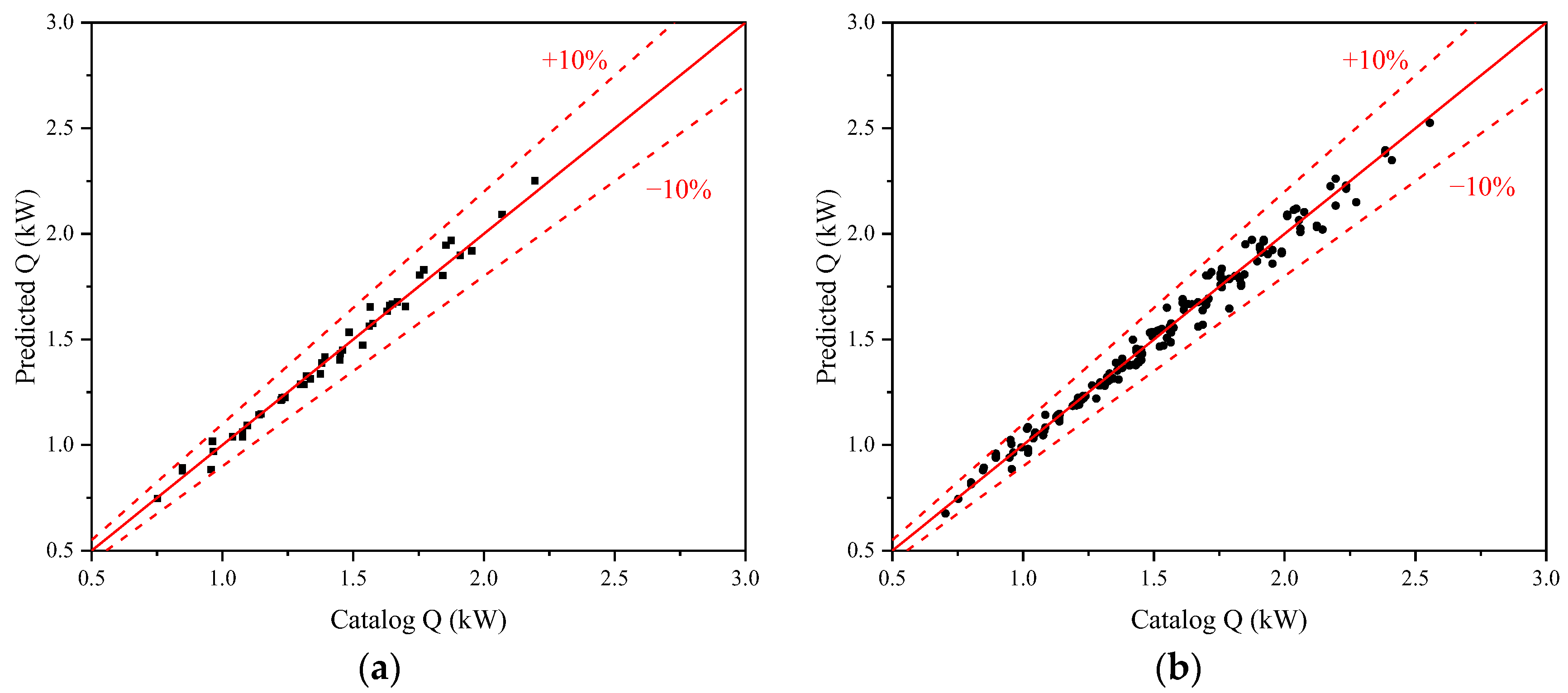
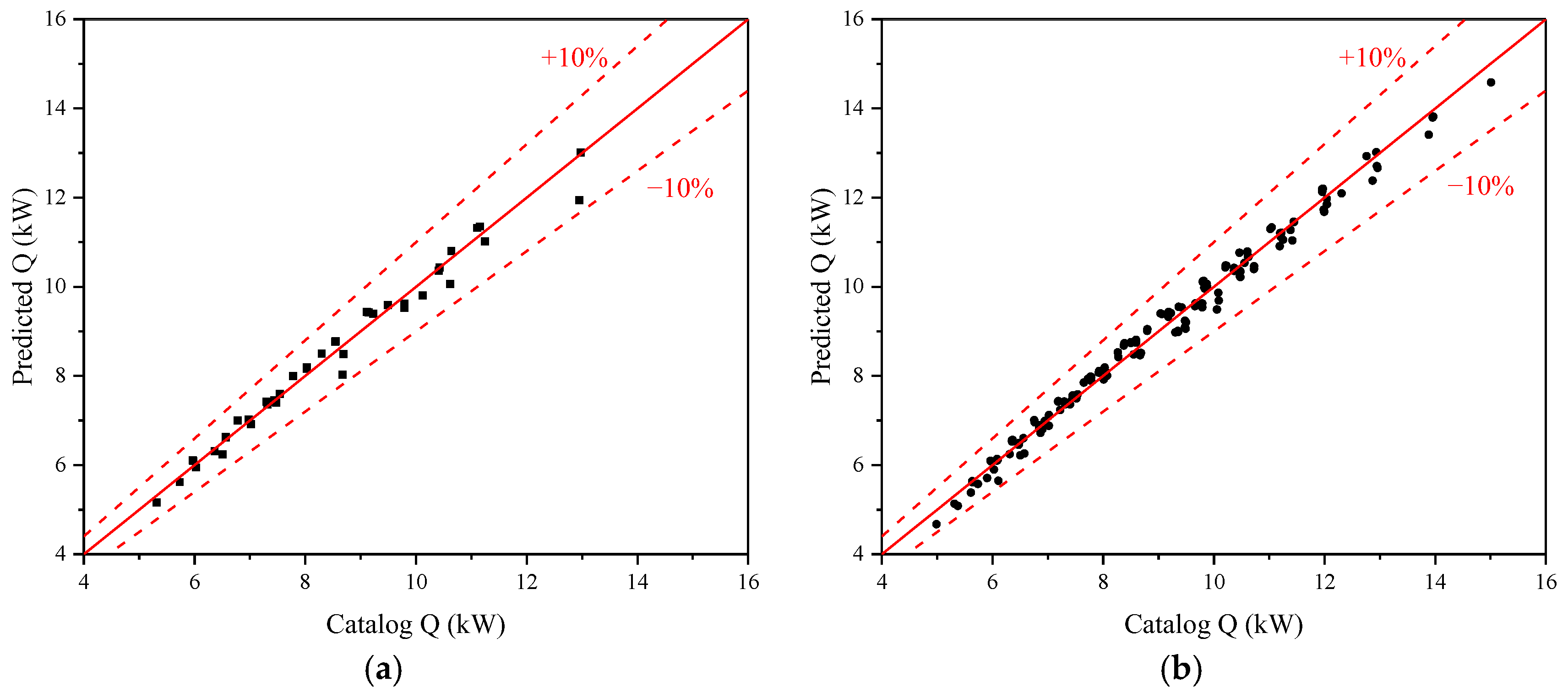
Based on the training and test datasets, the explicit calculation formula for each FCU model can be identified and tested. Take the models no. 200 and no. 1400, for example. Figure 3 compares the predicted and cataloged total cooling capacity of the FCU model no. 200 for the two sets, respectively. Figure 4 depicts the comparison for the model no. 1400. In the scatter plots, every black point represents an operating condition; the red solid and dotted lines refer to the relative error limits of 0%, −10%, and +10% to the catalog data. It can be observed that all points fall close to the 0% error line and between the ±10% error lines for both training and test sets. The total cooling capacity predicted by the proposed formula matches the catalog data well across all the operation conditions. It performs consistently from the training to the test datasets, indicating the formula’s accuracy and generalizability.
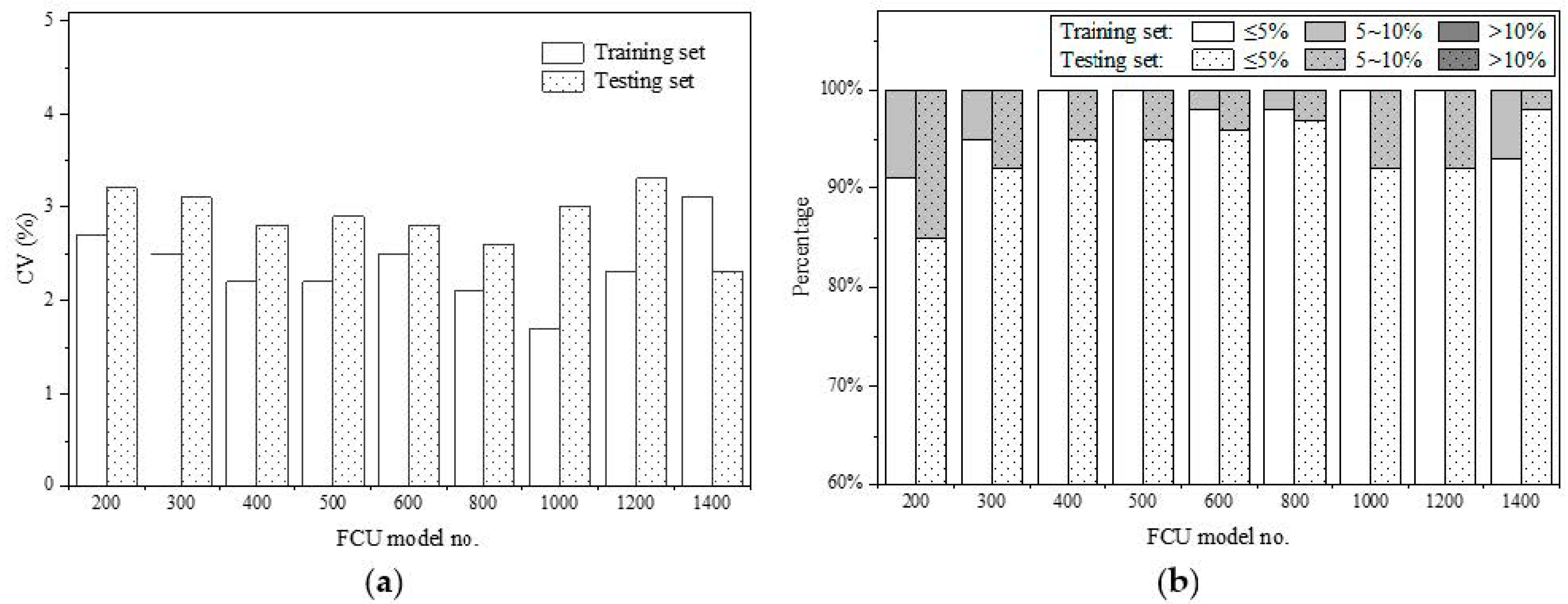
Table 3 lists the formulas’ identified parameters and overall accuracy indicators for all 9 FCU coils. Figure 5 depicts the CV values and relative error distribution of the prediction by the formulas. For the training sets, the CV values are about 2%, over 90% of points have a relative error of less than 5% (i.e., the average of P 5 is about 97%), and all points have a relative error of less than 10% (i.e., P 10 values). For the test sets, the CV and P 5 indicators degrade very slightly, i.e., the CV values are about 3%, and the average of P 5 is about 94%, but still, all points are within 10% error. The results indicate that the formula is robust for the series coils, from small nominal capacity to large capacity.

3.3. AHU Cooling Coils

Unlike FCU product catalogs, only one or two pieces of nominal cooling performance data are usually in AHU catalogs. They cannot directly support the validation approach like FCU coils. Therefore, we use a known coil model to generate the performance data of AHU coils for validation. The coil model is based on the classical temperature-based ε-NTU method, and it needs the technical parameters of the coils and heat transfer correlations obtained from experiments. The engineering handbook [49] provides some series AHU coils to meet the needs. We selected JW series coils from the handbook in the study since they have been adopted by DeST [39,54] and can be directly used to simulate the coil performance data.
The JW series coils have 4 coil types (JW10, JW20, JW30, JW40) and 3 kinds of tube rows (4 rows, 6 rows, and 8 rows), 12 coil models in total. We denote them by JW10_4R, JW10_6R, JW20_4R, etc. in the following. Table 4 shows an example of the JW20 6-row coil and lists the coil’s technical parameters and empirical correlations. With the information, the total cooling capacity of the coil can be iteratively calculated by the temperature-based ε-NTU method, given the inlet air and water conditions. Then, the simulated total capacity data are used as the benchmark for the training and test of the proposed formula.
According to the recommended conditions for the empirical correlations of JW series coils, we selected 216 conditions, including 3 levels of inlet chilled water temperature, 3 levels of water flow rate, 4 levels of air flow rate, 3 levels of inlet air dry-bulb temperature, and 2 levels of inlet air relative humidity, to train the proposed formula. For the test dataset, we use an interpolation method to construct the new conditions of the inlet water temperatures, water flow rates, and airflow rates, and use the air temperature and humidity data from Beijing’s typical meteorological year (TMY) weather data [54,55] in the summer, from 1 May to 30 September, to increase the new conditions of the inlet air dry-bulb temperature and humidity, to represent the coils working over a wide operating range. To ensure the AHU coils operate in wet conditions, we selected the TMY weather data where the air dry-bulb is higher than 26 °C and the air humidity is higher than 40%, i.e., 815 points. Table 5 details the training and test sets for validating the formula for AHU coils. Figure 6 depicts the inlet air conditions for the training and test sets. Overall, the test set has 500 times more data than the training set.
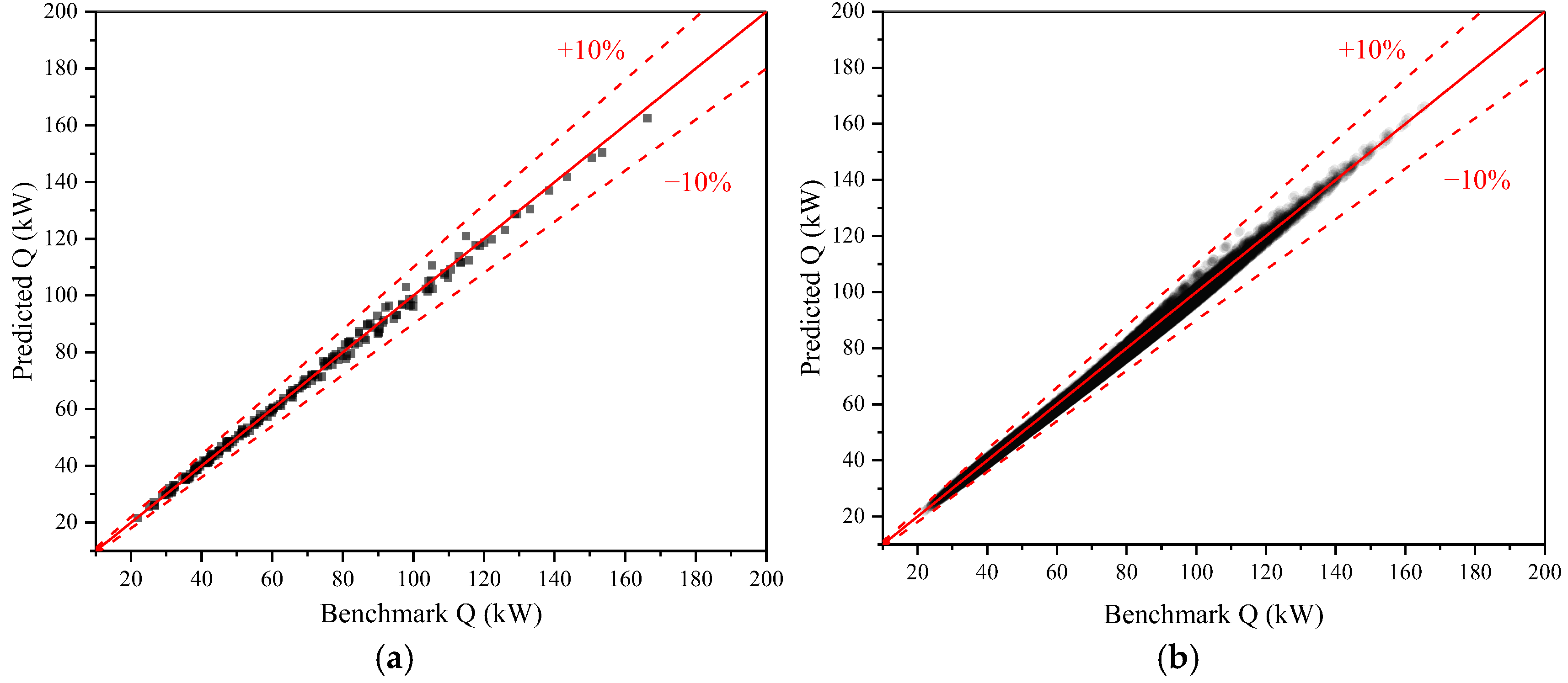
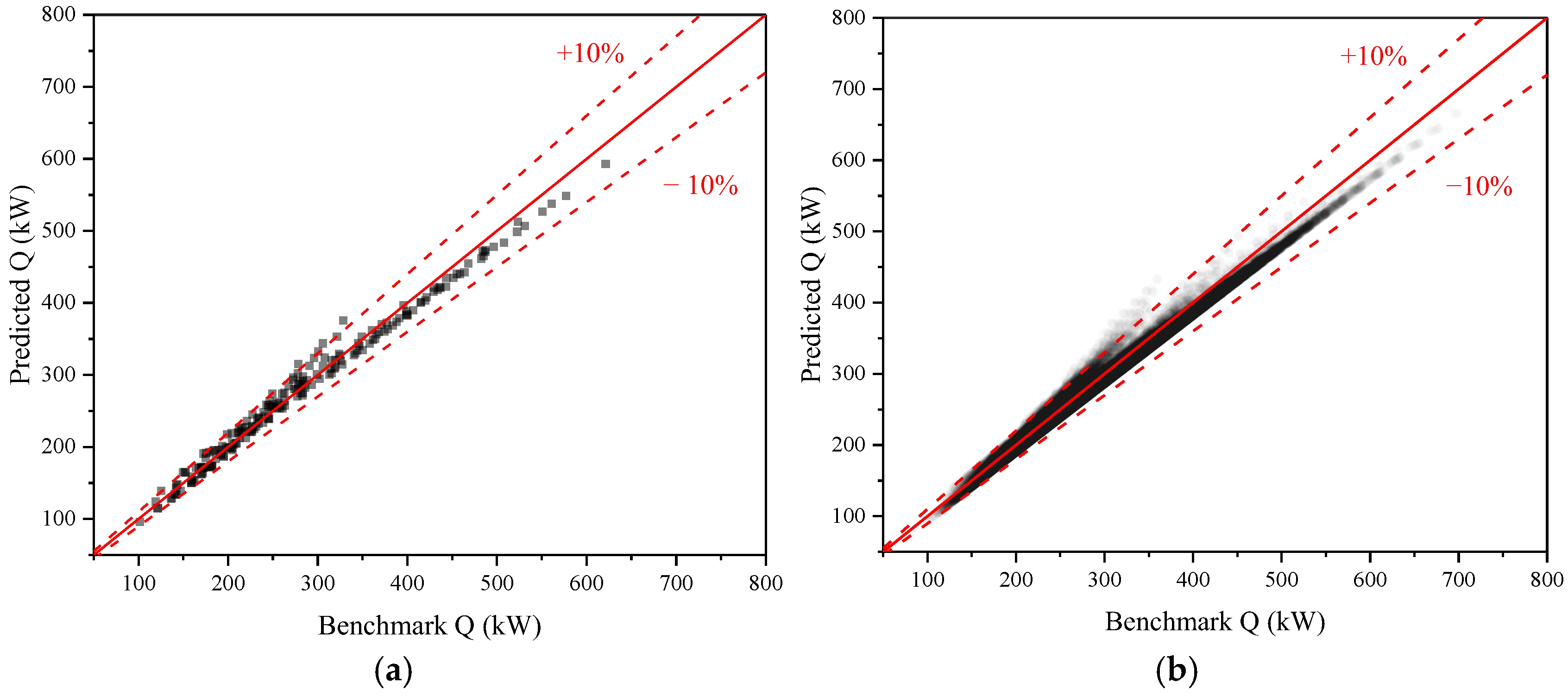
The proposed formula for each AHU coil was identified using the training set and tested using the test set. Take the coil JW10_4R and JW40_8R as examples. Figure 7 compares the predicted and benchmark total cooling capacity of JW10_4R for the two sets. Figure 8 depicts the comparison for JW40_8R. In the scatter plots, every black point represents an operating condition; the red solid and dotted lines refer to the relative error limits of 0%, −10%, and +10% to the benchmark capacity. For the coil JW10_4R with a smaller capacity, all points fall close to the 0% error line and between the ±10% error lines for both training and test sets. The comparison results for the coil JW40_8R with a larger capacity are similar. The predicted total capacity by the new formula is close to that calculated by the classical coil model in most cases; a few points around 300 kW exceed the relative error limit of ±10%; however, the size of these points is very small and does not exceed 0.3%. This discrepancy will be discussed in the next section. Overall, the simple explicit formula can get very close to the classical method well across the wide operation conditions and perform consistently from the training set to the test set, indicating that the formula has good accuracy and generalizability.
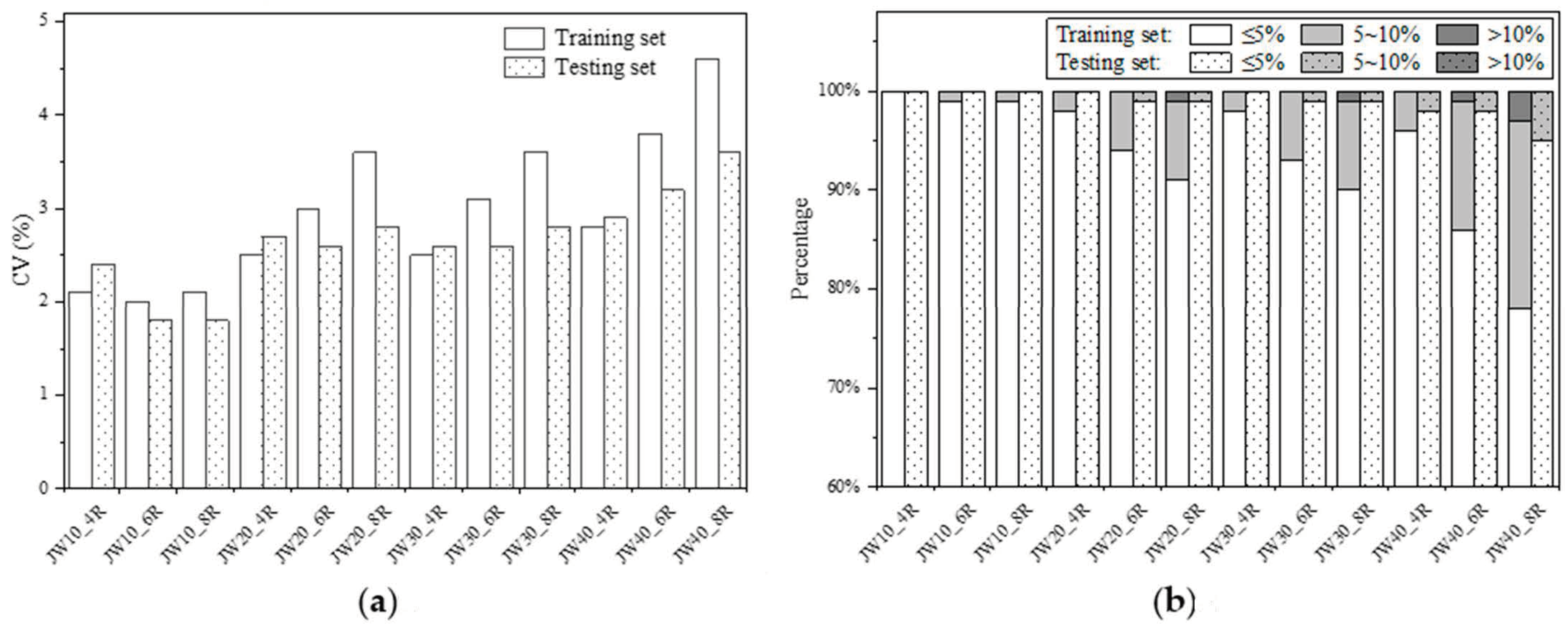
Table 6 lists all identified parameters and overall accuracy indicators of the formulas for all 12 AHU coils. Figure 9 depicts the CV values and relative error distribution of the prediction by the formulas. For the training sets, all the CV values are less than 5%, over 90% of points of 9 coils have a relative error of less than 5% (i.e., P 5 values), and nearly 100% of points of all coils have a relative error of less than 10% (i.e., P 10 values). For the test sets, the CV indicators of all coils remained mostly stable, i.e., nearly the same as those of the training sets; the P 5 and P 10 indicators of all coils got slightly better for all coils. Although a few points of 4 coils have a relative error of greater than 10%, the points are very tiny (less than 0.5%). Overall, the proposed formula performs with good accuracy and stability for the series AHU coils with various capacities and wide operation ranges.
Validation results on the FCU and AHU cooling coils show that the new explicit formula for calculating the total cooling capacity has high accuracy and generalizability for all the test cases, which would be essential for modeling the air-conditioning system in building energy simulation and control optimization.

4. Discussion

As shown in Figure 8 and 9b and Table 6, the proposed formula appeared to have a relative error of higher than 10% in some conditions comparing the performance data generated from the classical numerical AHU coil model when it was applied to the coils with six or eight tube rows (i.e., JW20_8R, JW30_8R, JW40_6R, and JW40_8R). The bias is mainly rooted in the cases of high moisture separation coefficients and small water flow rates. It might be an issue of the classical model since the classical coil model is based on empirical correlations that are fitted from experiment data and have a certain degree of errors. By consulting the original literature [56], we find that the classical AHU coil model’s error can reach over 20%. Since the literature did not list the original experimental data, we cannot compare our formula with them directly. Instead, we calculated the maximum deviations between the two models, i.e., about 16% for JW20_8R and JW30_8R, 17% for JW40_6R, and 21% for JW40_8R, and they are comparable with the inherent maximum error of the classical AHU coil model. Thus, although this discrepancy persists, we believe the generalizability of the formula can be stated. Further experimental data on AHU cooling coils will be needed to analyze and verify the issue.
The availability of the proposed explicit formula provides a much quicker method for evaluating the total cooling capacity of a chilled-water cooling coil under wet conditions compared to the classical implicit temperature-based or enthalpy-based coil models since it does not need any iteration. It would help improve computation efficiency in building energy simulation and control optimization.
Additionally, the explicit formula provides a new objective correlation for measuring the total performance of chilled-water cooling coils by experiments, which might help reduce the number of experimental conditions. As we can see, a small training set can have a close prediction performance compared to a large testing set, at least from the perspectives of the inlet water temperature (e.g., reduced from 5 levels to 2 levels for FCU coils and from 5 levels to 3 levels for AHU coils) and inlet air dry-bulb and humidity (e.g., reduced from 4 levels to 2 levels for FCU coils and from 815 levels to 6 levels for AHU coils), as shown in Table 2 and Table 5.

5. Conclusions

A simple explicit formula has been developed to evaluate the total capacity of chilled-water cooling coils under wet conditions. It is based on the principles of heat transfer and energy balance and the analogy to the empirical correlation of a forced flow’s overall heat transfer coefficient. It correlates the total capacity of a cooling coil to the air-side and water-side inlet conditions and has five variable parameters. Given the inlet air and water conditions, the total cooling capacity of the coil can be calculated immediately without any trial calculation or iteration. Therefore, it has a much faster computation speed than the classical implicit model of a wet cooling coil.
The new formula has been cross-validated using the catalog performance data of a series of FCU coils from the manufacturer and the generated performance data of a series of AHU coils from a well-established implicit ε-NTU model. By dividing the performance data of each coil into a training set with a smaller size and a test set with a larger size, i.e., the training set accounts for 20% for each FCU coil and 0.2% for each AHU coil, the formula exhibits a mean prediction error (i.e., CV value) of less than 5% in both sets of all the coils. Compared to the benchmark data from catalogs or classical models, all of the data points fall within a relative error range of ±10% for all FCU coils and most of the AHU coils, and only a very few points (less than 0.3%) exceed the 10% error limit for several AHU coils. This indicates that the formula has high accuracy and generalizability and the potential to obtain its five parameters with a small set of experiment conditions.
Overall, the formula has the advantages of a simple structure, fast calculation, and high accuracy when applied to the modeling of chilled-water-based air-cooling coils under wet conditions. A small issue is that the coil performance predicted by the formula and the implicit AHU cooling coil model do not match well in very few cases, so further experimental data will need to be analyzed in the future. Additional work includes building a complete cooling coil model for wet and dry conditions, integrating it into an annual building energy simulation software like DeST (Ver. 20230713), and exploring its feasibility in the control optimization and performance diagnosis of on-site air-conditioning system operation.

Author Contributions

Conceptualization, C.W. and J.A.; methodology, C.W., S.W., X.D. and J.A.; validation, S.W., X.D. and C.W.; writing—original draft preparation, C.W., S.W. and X.F.; writing—review and editing, C.W.; visualization, C.W., S.W. and X.D. All authors have read and agreed to the published version of the manuscript.

Funding

This work was supported by the National Natural Science Foundation of China (No. 51608297), the Scientific Research Project of Beijing Municipal Education Commission (No. KM201910016009 and No. KZ202110016022), BUCEA Pyramid Talent Training Project (No. JDYC20220815).

Data Availability Statement

Data will be made available on request.

Conflicts of Interest

The authors declare no conflicts of interest.

Nomenclature

Q total cooling capacity, in W; Q s sensible cooling capacity, in W;
m a air flow rate, in kg/s; m w water flow rate, in kg/s;
c a moist air-specific heat, in J/kg-K; c w water-specific heat, in J/kg-K;
t a , i air inlet dry-bulb temperature, in °C; t w , i water inlet temperature, in °C;
t a , o air outlet dry-bulb temperature, in °C; t w , o water outlet temperature, in °C;
h a , i air inlet enthalpy, in J/kg; h w , s a t , i saturated air enthalpy at the water inlet temperature, in J/kg;
h a , o air outlet enthalpy, in J/kg;
d a , i air inlet humidity, in g/kg; h w , s a t , o saturated air enthalpy at the water outlet temperature, in J/kg;
t s effective coil surface temperature, in °C;
h s , s a t saturated air enthalpy at the coil surface temperature, in J/kg; η o overall fin surface efficiency;
U a air-side thermal conductance, in W/(K·m2); U w water-side thermal conductance, in W/(K·m2);
A a air-side heat transfer area, in m2; A w water-side heat transfer area, in m2;
ε overall effectiveness of the coil; ε a air-side effectiveness of the coil;
U A h enthalpy-based overall thermal conductance, in W/(J/kg); U A temperature-based overall thermal conductance, in W/K;
Δ h L M log mean enthalpy difference, in J/kg; Δ t L M log mean temperature difference, in K;
c s fictitious specific heat; ξ moisture separation coefficient
C V coefficient of variation; R M S E root mean squared error;
P 5 relative prediction error proportion of the number of points to all operating points smaller than 5%; P 10 relative prediction error proportion of the number of points to all operating points smaller than 10%.

References

  1. Elmahdy, A.H.; Mitalas, G.P. A Simple Model for Cooling and Dehumidifying Coils for Use in Calculating Energy Requirements for Buildings. ASHRAE Trans. 1977, 83, 103–117. [Google Scholar]
  2. Braun, J.E. Methodologies for the Design and Control of Central Cooling Plants. Ph.D. Thesis, University of Wisconsin-Madison, Madison, WI, USA, 1988. [Google Scholar]
  3. Chow, T.T. Chilled water cooling coil models from empirical to fundamental. Numer. Heat Transf. Part A Appl. 1997, 32, 63–83. [Google Scholar] [CrossRef]
  4. Vardhan, A.; Dhar, P.L. A New Procedure for Performance Prediction of Air Conditioning Coils. Int. J. Refrig. 1998, 21, 77–83. [Google Scholar] [CrossRef]
  5. Zhou, X.; Braun, J.E. Transient Modeling of Chilled Water Cooling Coils. In Proceedings of the International Refrigeration and Air Conditioning Conference, West Lafayette, IN, USA, 12–15 July 2004. [Google Scholar]
  6. Yao, Y.; Lian, Z.; Hou, Z. Thermal Analysis of Cooling Coils Based on a Dynamic Model. Appl. Therm. Eng. 2004, 24, 1037–1050. [Google Scholar] [CrossRef]
  7. Wang, Y.-W.; Cai, W.-J.; Soh, Y.-C.; Li, S.-J.; Lu, L.; Xie, L. A Simplified Modeling of Cooling Coils for Control and Optimization of HVAC Systems. Energy Convers. Manag. 2004, 45, 2915–2930. [Google Scholar] [CrossRef]
  8. Khamis, M.; Hassab, M. Thermal Design of Cooling and Dehumidifying Coils. In Heat Exchangers—Basics Design Applications; Mitrovic, J., Ed.; InTech: Houston, TX, USA, 2012; ISBN 978-953-51-0278-6. [Google Scholar]
  9. Song, L.; Wang, G. Using a Hybrid Method to Construct a Computational Efficient Cooling Coil Model for an Automated Single-Duct Variable Air Volume System Fault Detection and Diagnosis. Energy Build. 2015, 92, 363–373. [Google Scholar] [CrossRef]
  10. Nazari, M.; Ghaffari, A. Modeling and Analysis of Cooling Coil for Control System Design Using Gray Box Approach. Mod. Appl. Sci. 2016, 10, 23. [Google Scholar] [CrossRef]
  11. Liao, H.; Cai, W.; Cheng, F.; Dubey, S.; Rajesh, P.B. An Online Data-Driven Fault Diagnosis Method for Air Handling Units by Rule and Convolutional Neural Networks. Sensors 2021, 21, 4358. [Google Scholar] [CrossRef] [PubMed]
  12. Yin, P.; Alam, T.; O’Neal, D. Empirical Modeling of Variable Air Variable Water Fan Coil Units in Cooling Mode for Building Energy Calculations (RP-1741). ASHRAE Trans. 2019, 125, 49–52. [Google Scholar]
  13. Morisot, O.; Marchio, D.; Stabat, P. Simplified Model for the Operation of Chilled Water Cooling Coils Under Nonnominal Conditions. HVAC&R Res. 2002, 8, 135–158. [Google Scholar] [CrossRef]
  14. Rabehl, R.; Mitchell, J.; Beckman, W. Parameter Estimation and the Use of Catalog Data in Modeling Heat Exchangers and Coils. HVAC&R Res. 1999, 5, 3–17. [Google Scholar] [CrossRef]
  15. Yan, C.; Yang, X.; Xu, Y. Mathematical Explanation and Fault Diagnosis of Low Delta-T Syndrome in Building Chilled Water Systems. Buildings 2018, 8, 84. [Google Scholar] [CrossRef]
  16. Wang, C.-C.; Chang, C.-T. Heat and Mass Transfer for Plate Fin-and-Tube Heat Exchangers, with and without Hydrophilic Coating. Int. J. Heat Mass Transf. 1998, 41, 3109–3120. [Google Scholar] [CrossRef]
  17. Wang, J.; Hihara, E. Prediction of Air Coil Performance under Partially Wet and Totally Wet Cooling Conditions Using Equivalent Dry-Bulb Temperature Method. Int. J. Refrig. 2003, 26, 293–301. [Google Scholar] [CrossRef]
  18. Yu, X.; Wen, J.; Smith, T.F. A Model for the Dynamic Response of a Cooling Coil. Energy Build. 2005, 37, 1278–1289. [Google Scholar] [CrossRef]
  19. Wang, G.; Liu, M.; Claridge, D.E. Decoupled Modeling of Chilled Water Cooling Coils Using a Finite Element Method. In Proceedings of the Fifth International Conference for Enhanced Building Operations, Pittsburgh, PA, USA, 11–13 October 2005. [Google Scholar]
  20. Zhou, X.; Braun, J. A Simplified Dynamic Model for Chilled-Water Cooling and Dehumidifying Coils—Part 1: Development (RP-1194). HVAC&R Res. 2007, 13, 785–804. [Google Scholar] [CrossRef]
  21. Li, P.; Li, Y.; Seem, J. Modelica-Based Dynamic Modeling of a Chilled-Water Cooling Coil. HVAC&R Res. 2010, 16, 35–58. [Google Scholar] [CrossRef]
  22. Stoecker, W.F. Procedures for Simulating the Performance of Components and Systems for Energy Calculations, 3rd ed.; U.S. Department of Energy Office of Scientific and Technical Information: Oak Ridge, TN, USA, 1975. [Google Scholar]
  23. De La Cruz-Loredo, I.; Zinsmeister, D.; Licklederer, T.; Ugalde-Loo, C.E.; Morales, D.A.; Bastida, H.; Perić, V.S.; Saleem, A. Experimental Validation of a Hybrid 1-D Multi-Node Model of a Hot Water Thermal Energy Storage Tank. Appl. Energy 2023, 332, 120556. [Google Scholar] [CrossRef]
  24. Bell, I.H.; Quoilin, S.; Georges, E.; Braun, J.E.; Groll, E.A.; Horton, W.T.; Lemort, V. A Generalized Moving-Boundary Algorithm to Predict the Heat Transfer Rate of Counterflow Heat Exchangers for Any Phase Configuration. Appl. Therm. Eng. 2015, 79, 192–201. [Google Scholar] [CrossRef]
  25. Heinz, A.; Lerch, W.; Heimrath, R. Heat Pump Condenser and Desuperheater Integrated into a Storage Tank: Model De-velopment and Comparison with Measurements. Appl. Therm. Eng. 2016, 102, 465–475. [Google Scholar] [CrossRef]
  26. Cadafalch, J.; Carbonell, D.; Consul, R.; Ruiz, R. Modelling of Storage Tanks with Immersed Heat Exchangers. Sol. Energy 2015, 112, 154–162. [Google Scholar] [CrossRef]
  27. Ren, C.; Yang, H. An Analytical Model for the Heat and Mass Transfer Processes in Indirect Evaporative Cooling with Parallel/Counter Flow Configurations. Int. J. Heat Mass Transf. 2006, 49, 617–627. [Google Scholar] [CrossRef]
  28. Xia, L.; Chan, M.Y.; Deng, S.M.; Xu, X.G. Analytical Solutions for Evaluating the Thermal Performances of Wet Air Cooling Coils under Both Unit and Non-Unit Lewis Factors. Energy Convers. Manag. 2010, 51, 2079–2086. [Google Scholar] [CrossRef]
  29. Xia, L.; Chan, M.Y.; Deng, S.M.; Xu, X.G. A Modified Logarithmic Mean Enthalpy Difference (LMED) Method for Evaluating the Total Heat Transfer Rate of a Wet Cooling Coil under Both Unit and Non-Unit Lewis Factors. Int. J. Therm. Sci. 2009, 48, 2159–2164. [Google Scholar] [CrossRef]
  30. Lee, C.K. A Simplified Explicit Model for Determining the Performance of a Chilled Water Cooling Coil. Int. J. Refrig. 2014, 43, 167–175. [Google Scholar] [CrossRef]
  31. Wetter, M. Simulation Model Finned Water-to-Air Coil without Condensation; Lawrence Berkeley National Laboratory: Berkeley, CA, USA, 1999. [Google Scholar]
  32. Lemort, V.; Lebrun, J.; Cuevas, C.; Teodorese, I.V. Development of Simple Cooling Coil Models for Simulation of HVAC Systems. ASHRAE Trans. 2008, 114, 319–328. [Google Scholar]
  33. Bertagnolio, S.; Lebrun, J. Simulation of a Building and Its HVAC System with an Equation Solver: Application to Benchmarking. Build. Simul. 2008, 1, 234–250. [Google Scholar] [CrossRef]
  34. Xia, L.; Yang, T.; Chan, Y.; Tang, L.; Chen, Y.-T. Optimisation of Direct Expansion (DX) Cooling Coils Aiming to Building Energy Efficiency. J. Build. Constr. Plan. Res. 2015, 03, 47–59. [Google Scholar] [CrossRef]
  35. Mansour, M.K.; Fath, H.E. A New and Practical ε-NTU Correlation for the Humidification Process under Different Lewis Number. Desalination 2016, 395, 72–78. [Google Scholar] [CrossRef]
  36. Mansour, M.K.; Hassab, M.A. Simplified Approach of Predictions of Thermal Performance for Counterflow Fully-Wet Cooling Coil. Heat Mass Transf. 2017, 53, 2211–2217. [Google Scholar] [CrossRef]
  37. Ruivo, C.R.; Dominguez-Muñoz, F.; Costa, J.J. Simplified Model of Finned-Tube Heat Exchangers Based on the Effectiveness Method and Calibrated with Manufacturer and Experimental Data. Appl. Therm. Eng. 2017, 111, 340–352. [Google Scholar] [CrossRef]
  38. Mitchell, J.W.; Braun, J.E. Principles of Heating, Ventilation, and Air Conditioning in Buildings, 1st ed.; Wiley: Hoboken, NJ, USA, 2012; ISBN 978-0-470-62457-9. [Google Scholar]
  39. Yan, D.; Xia, J.; Tang, W.; Song, F.; Zhang, X.; Jiang, Y. DeST—An Integrated Building Simulation Toolkit Part I: Fundamentals. Build. Simul. 2008, 1, 95–110. [Google Scholar] [CrossRef]
  40. U.S. Department of Energy. EnergyPlus Version 23.1: Engineering Reference; U.S. Department of Energy: Washington, DC, USA, 2023. [Google Scholar]
  41. Thermal Energy System Specialists, LLC. TRNSYS 18: Mathematical Reference; Thermal Energy System Specialists, LLC.: Madison, WI, USA, 2019. [Google Scholar]
  42. Zendehboudi, A. Experimental Analysis of a Tri-Partite Brazed Plate Gas Cooler for CO2 Heat Pump Water Heaters. Appl. Therm. Eng. 2024, 241, 122376. [Google Scholar] [CrossRef]
  43. Lian, Z.; Chen, B. Fundamentals & Equipment of Heat & Mass Transfer, 4th ed.; China Architecture & Building Press: Beijing, China, 2018. [Google Scholar]
  44. Zhao, R.; Fan, C.; Xue, D.; Qian, Y. Air Conditioning, 4th ed.; China Architecture & Building Press: Beijing, China, 2009. [Google Scholar]
  45. Jin, G.-Y.; Cai, W.-J.; Wang, Y.-W.; Yao, Y. A Simple Dynamic Model of Cooling Coil Unit. Energy Convers. Manag. 2006, 47, 2659–2672. [Google Scholar] [CrossRef]
  46. Virtanen, P.; Gommers, R.; Oliphant, T.E.; Haberland, M.; Reddy, T.; Cournapeau, D.; Burovski, E.; Peterson, P.; Weckesser, W.; Bright, J.; et al. SciPy 1.0: Fundamental Algorithms for Scientific Computing in Python. Nat. Methods 2020, 17, 261–272. [Google Scholar] [CrossRef] [PubMed]
  47. Gao, F.; Han, L. Implementing the Nelder-Mead Simplex Algorithm with Adaptive Parameters. Comput. Optim. Appl. 2012, 51, 259–277. [Google Scholar] [CrossRef]
  48. GB/T 19232-2003; Ministry of Construction of P.R. China. National Standard: Fan Coil Units. China Architecture & Building Press: Beijing, China, 2003.
  49. Lu, Y. Practical Design Handbook for Heating and Air-Conditioning, 2nd ed.; China Architecture & Building Press: Beijing, China, 2008. [Google Scholar]
  50. Zhang, B.; You, S.; Wang, S.; Ding, X.; Wang, C.; Gao, Y. From Laboratory to On-Site Operation: Reevaluation of Empirically Based Electric Water Chiller Models. Build. Simul. 2022, 15, 213–232. [Google Scholar] [CrossRef]
  51. Palaić, D.; Štajduhar, I.; Ljubic, S.; Wolf, I. Development, Calibration, and Validation of a Simulation Model for Indoor Temperature Prediction and HVAC System Fault Detection. Buildings 2023, 13, 1388. [Google Scholar] [CrossRef]
  52. Talib, R.; Nabil, N.; Choi, W. Optimization-Based Data-Enabled Modeling Technique for HVAC Systems Components. Buildings 2020, 10, 163. [Google Scholar] [CrossRef]
  53. Shanghai SINKO Co. Ltd. SINKO Fan Coil Unit—SGCR2006A Series Catalog (Following GB/T19232-2003). 2015, p. 490. Available online: https://wenku.baidu.com/view/f4f98a03ec3a87c24128c47e.html (accessed on 11 July 2024).
  54. Tsinghua DeST Group. DeST—Designer’s Simulation Toolkit. 2024. Available online: https://www.dest.net.cn/ (accessed on 11 July 2024).
  55. Wang, C.; Li, X.; Sun, W.; An, J.; Gao, S. Occupant Behavior, Thermal Environment, and Appliance Electricity Use of a Single-Family Apartment in China. Sci. Data 2024, 11, 65. [Google Scholar] [CrossRef]
  56. Zhang, Y.; Xue, D. Enthalpy efficiency method for air cooling coils on wet conditions. Chinese Journal of Refrigeration. 1984, 4, 33–42. (In Chinese) [Google Scholar]
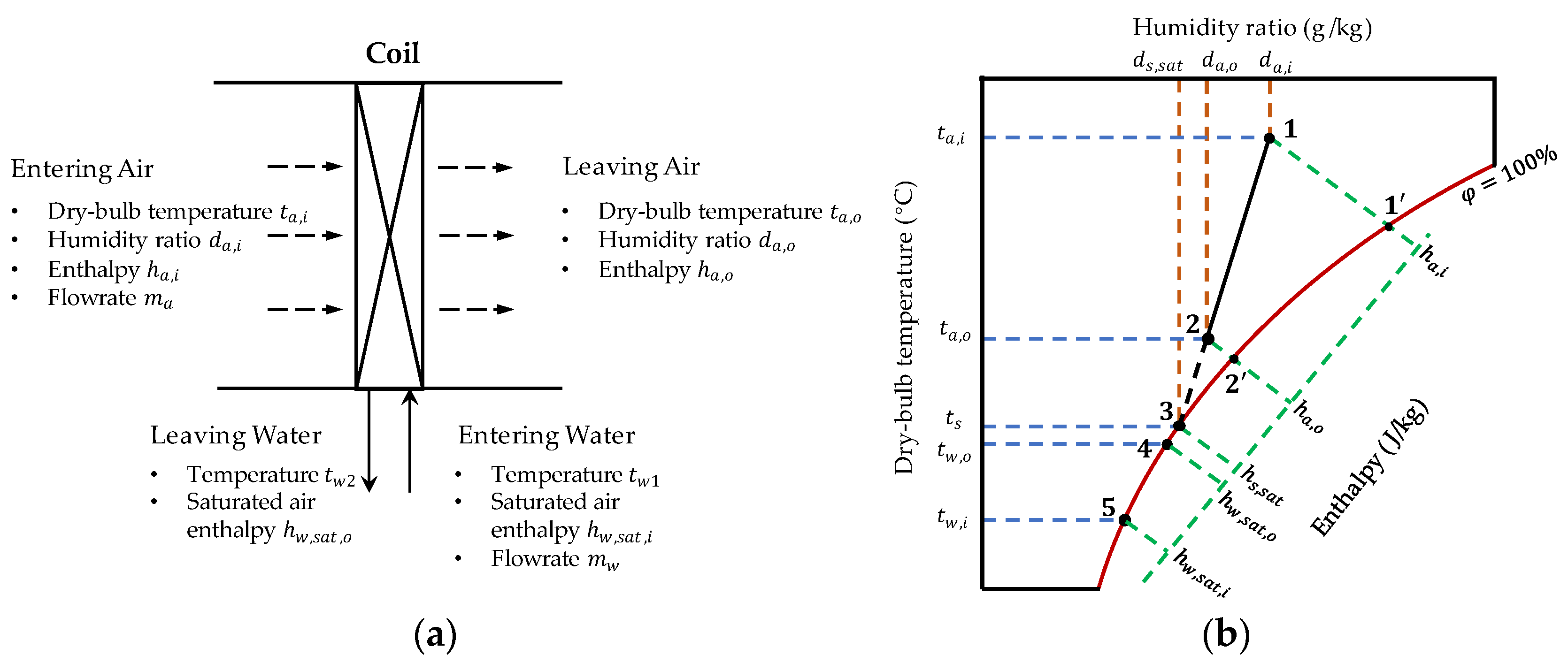
Figure 1. Lumped scheme of a cooling and dehumidifying coil: (a) Flow paths and inlet/outlet conditions; (b) Psychrometric process.
Buildings 14 02630 g001
Figure 2. Property profiles and energy flows in a wet cooling coil (modified from [38]): (a) Property profiles in the air stream; (b) Energy flows in the wet section.
Buildings 14 02630 g002
Figure 3. Predicted vs. catalog values of total cooling capacity of FCU model no. 200: (a) Training set; (b) Test set.
Buildings 14 02630 g003
Figure 4. Predicted vs. catalog values of total cooling capacity of FCU model no. 1400: (a) Training set; (b) Test set.
Buildings 14 02630 g004
Figure 5. Overall prediction accuracy of the formulas for series FCU coils: (a) Coefficient of variation; (b) Relative error distribution.
Buildings 14 02630 g005
Figure 6. Inlet air conditions for the training and test datasets.
Buildings 14 02630 g006
Figure 7. Predicted vs. benchmark total cooling capacity of AHU JW10_4R: (a) Training set; (b) Test set.
Buildings 14 02630 g007
Figure 8. Predicted vs. benchmark total cooling capacity of AHU JW40_8R: (a) Training set; (b) Test set.
Buildings 14 02630 g008
Figure 9. Overall prediction accuracy of the formula for JW series coils: (a) Training set; (b) Test set.
Buildings 14 02630 g009
Table 1. Enthalpy-based vs. temperature-based ε-NTU methods.
Equation TypeEnthalpy-Based ε-NTU MethodTemperature-Based ε-NTU Method
Total capacity Q = m a h a , i h a , o = m w c w ( t w , o t w , i )
Sensible capacity Q s = m a c a t a , i t a , o
Overall effectiveness Q = U A h Δ h L M Q = U A Δ t L M
c s = d h w , s a t d t w t w = h w , s a t , i h w , s a t , o t w , i t w , o ξ = 1 c a d h a d t a x = Q Q s = h a , i h a , o c a ( t a , i t a , o )
For wet conditions, ξ > 1 .
U A h = c a η o U a A a + c s U w A w 1 U A = 1 η o U a A a + 1 U w A w 1 = f ( ξ , V a , V w )
N T U = U A h m a
C r = m a c s m w c w
ε = h a , i h a , o h a , i h w , s a t , i
N T U = U A ξ m a c a
C r = ξ m a c a m w c w
ε = t a , i t a , o t a , i t w , i
ε = 1 e x p [ N T U 1 C r ] 1 C r e x p [ N T U 1 C r ] (e.g., for counterflow cooling coils)
Air-side effectiveness (or contact effectiveness [32,43,44]) N T U a = η o U a A a m a c a
ε a = t a , i t a , o t a , i t s = h a , i h a , o h a , i h s , s a t = 1 exp N T U a = f ( V a )
Table 2. Operation conditions in FCU catalog performance tables and the selected training set.
ParameterAll Operation ConditionsTraining Set
Inlet water temperature (°C)Five levels: 5, 6, 7, 8, 9Two levels: 6, 8
Water flow rate (L/min)Four levels that differ with model number, i.e.,
2.4, 4.8, 6, 7.2 for model no. 200;
3.6, 4.8, 7.2, 9.6 for model no. 300;
4.8, 7.2, 9.6, 12 for model no. 400;
6.0, 9.6, 13.2, 15.6 for model no. 500;
7.2, 12, 15, 18 for model no. 600;
12, 15.6, 19.2, 24 for model no. 800;
14.4, 18, 24, 30 for model no. 1000;
18, 24, 30, 33 for model no. 1200;
18, 24, 30, 39 for model no. 1400.
All four levels
Inlet air dry and wet bulb temperature (°C)Four levels: (24, 17), (25, 17.8), (26, 18.7), (27, 19.5)Two levels: (24, 17), (26, 18.7)
Air flow rate (m3/h)Three levels that differ with model number, i.e.,
195, 280, 360 for model no. 200;
290, 415, 550 for model no. 300;
380, 560, 720 for model no. 400;
450, 675, 900 for model no. 500;
545, 765, 1040 for model no. 600;
755, 1090, 1450 for model no. 800;
910, 1355, 1800 for model no. 1000;
1095, 1650, 2180 for model no. 1200;
1550, 2050, 2600 for model no. 1400.
All three levels
Number of operation states 5 × 4 × 4 × 3 = 240 2 × 4 × 2 × 3 = 48
(20%)
Table 3. Parameter and evaluation indicators for the series FCU coils.
FCU No.Training SetTest Set
a 1 b 1 e 1 a 2 b 2 CV P 5 P 10 CV P 5 P 10
2000.499−0.5021.15227.7660.0322.7%91%100%3.2%85%100%
3000.606−0.7071.15728.5100.0982.5%95%100%3.1%92%100%
4001.294−0.5510.96736.6330.0312.2%100%100%2.8%95%100%
5001.061−0.5290.98138.9310.0442.2%100%100%2.9%95%100%
6001.552−0.4900.91149.894−0.0262.5%98%100%2.8%96%100%
8002.335−0.6020.89241.2530.1222.1%98%100%2.6%97%100%
10002.138−0.5270.88747.0940.0461.7%100%100%3.0%92%100%
12003.088−0.5070.82553.2540.0282.3%100%100%3.3%92%100%
14000.166−0.4921.20054.2310.0183.1%93%100%2.3%98%100%
Table 4. Technical parameters and empirical correlations of JW20 6-row coil.
InformationValue
Tube-fin surface area of each row (m2)24.05
Airflow windward area (m2)1.87
Waterflow crossing area (m2)0.00407
Overall thermal conductance (W/m2-K) K = 1 41.5 V y 0.52 ξ 1.02 + 1 325.6 w 0.8 1
Air-side effectiveness ε = 0.0454 V y + 1.0049
Table 5. Information on the training and test datasets for AHU coils.
ParameterTraining DatasetTest Dataset
Number of LevelsValuesNumber of LevelsValues
Inlet water temperature (°C)35, 7, 955, 6, 7, 8, 9
Water velocity (m/s)30.6, 1.2, 1.870.6, 0.8, 1, 1.2, 1.4, 1.6, 1.8
Air velocity (m/s)41.5, 2, 2.5, 341.8, 2.1, 2.4, 2.7
Inlet air dry-bulb temperature (°C)328, 30, 32815Beijing TMY weather data in summer [54]
(>26 °C, >40%)
Inlet air relative humidity (%)240, 80
Number of operation states216
(<0.2%)
114,100
Table 6. Parameter and evaluation indicators for the series AHU cooling coils.
AHU No.Training SetTest Set
a 1 b 1 e 1 a 2 b 2 CV P 5 P 10 CV P 5 P 10
JW10_4R0.6150.1720.7182.323−0.3042.1%99.5%100.0%2.4%99.9%100.0%
JW10_6R0.9650.0470.8062.993−0.2372.0%99.1%100.0%1.8%100.0%100.0%
JW10_8R0.9670.0420.8494.085−0.2482.1%98.6%100.0%1.8%99.9%100.0%
JW20_4R0.8410.1480.7272.832−0.2402.5%97.5%100.0%2.7%99.5%100.0%
JW20_6R1.416−0.0140.8123.331−0.1843.0%93.8%100.0%2.6%99.4%100.0%
JW20_8R1.422−0.0270.8573.945−0.1783.6%90.6%98.6%2.8%98.9%99.9%
JW30_4R0.9480.1360.7323.021−0.2352.5%97.5%100.0%2.6%99.7%100.0%
JW30_6R1.539−0.0220.8163.552−0.1813.1%92.9%100.0%2.6%99.4%100.0%
JW30_8R1.519−0.0340.8604.194−0.1753.6%89.7%98.6%2.8%98.8%99.9%
JW40_4R1.1450.1120.7403.113−0.2122.8%95.9%100.0%2.9%98.3%100.0%
JW40_6R2.097−0.0900.8263.493−0.1643.8%86.4%99.0%3.2%98.0%99.9%
JW40_8R2.126−0.1160.8763.920−0.1584.6%78.1%96.7%3.6%95.4%99.7%
Disclaimer/Publisher’s Note: The statements, opinions and data contained in all publications are solely those of the individual author(s) and contributor(s) and not of MDPI and/or the editor(s). MDPI and/or the editor(s) disclaim responsibility for any injury to people or property resulting from any ideas, methods, instructions or products referred to in the content.