A Real-Time Inverted Velocity Model for Fault Detection in Deep-Buried Hard Rock Tunnels Based on a Microseismic Monitoring System

Abstract

Microseismic monitoring is an effective and widely used technology for dynamic fault disaster early warning and prevention in deep-buried hard rock tunnels. However, the insufficient understanding of the distribution of native faults poses a major challenge to yielding precise early warnings of disasters using an MS (Microseismic Monitoring System). Velocity field inversion is a reliable means to reflect fault information, and there is an urgent need to establish a real-time velocity field inversion method during tunnel excavation. In this paper, a method based on an MS is proposed to achieve the inversion of the velocity field in the monitoring area using microseismic event and excavation blasting data. The velocity field inversion method integrates the reflected wave ray-tracing method based on PSO (Particle Swarm Optimization) theory and FWI (Full-Waveform Inversion) theory. The accuracy of the proposed velocity inversion method was verified by various classic numerical simulation cases. In numerical simulations, the robustness of our method is evident in its ability to identify anomalous structural surfaces and velocity discontinuities ahead of the tunnel face.

1. Introduction

Currently, an increasing number of deep-buried tunnels are being utilized for transportation, hydropower, mining, and energy storage, among other purposes. The geological environment of deep rock engineering is extremely complex, influenced by the strong coupling effects of internal and external forces within the Earth’s multiple layers, and it exhibits susceptibility to severe forms of geological disasters such as water and mud outbursts, high-intensity rock bursts, etc. With the increase in tunnel burial depth, the increasing frequency of rock burst incidents seriously affects construction progress and operational safety, leading to a series of safety hazards including casualties, equipment damage, delays in project completion, and project failure [1,2].

The occurrence of fault disasters such as rock bursts is the result of the combined effects of excavation disturbance and the development of fault fissures. We can use mechanical behavior analysis and relevant statistical methods to predict and simulate the impact of excavation disturbance [3,4,5]. For the dynamic development of faults, we can use some in-situ monitoring methods. Microseismic monitoring technology is an effective technique for the monitoring and early warning of rock mass failure, and is considered crucial for obtaining premonitory information on rock fracture to predict rock burst risk. It has been widely used in deep rock engineering [6,7]. Previous studies have indicated that the occurrence of instantaneous rockbursts near fault zones and fractured zones tend to have a higher intensity, often resulting in larger “V”-shaped blast craters [8]. The spatial evolution of microseismic events indicates that cracks initially propagate along the structural surface, and eventually slide and fail along the surface [9]. The presence of structural surfaces is the dominant factor triggering such disasters. However, these conclusions are mostly drawn from post-exposure fault analysis. In other words, if we can master information in advance on native faults during microseismic monitoring and combine it with new seismic events, we can effectively improve the accuracy of fault disaster early warning. Therefore, understanding the distribution of forward faults ahead of the tunnel face is a crucial task for an MS.

Geophysical methods primarily involve the identification of fault geological bodies by utilizing differences in the velocity fields of waves. They were first applied in the field of Earth sciences. The scholars initially used a regular linear observation method to interpret plate tectonics based on seismic profiles. Dickmann proposed the concept of tunnel geophysics based on this approach [10]. Shortly after, the Swiss company Amberg introduced the TSP (Tunnel Seismic Prediction) series of products, leading to a gradual rise in the popularity of advance geological forecasting [11]. The theoretical basis of TSP involves scanning the velocity field of the seismic source profile with small-aperture borehole sensors, followed by Kirchhoff migration or reverse-time migration using the scanned velocity field to achieve imaging of geological bodies in front of the tunnel face [12,13,14].

However, the large-scale application of the TSP method has also brought about some difficulties and challenges. For example, the repeated triggering of explosive sources during geophysical exploration may damage the integrity of the rock mass at the site, leading to increased maintenance costs in the later stages due to the development of fractures in the surrounding rock mass caused by the vibrations [15]. In addition, the geophysical exploration process takes a considerable amount of time, which has a certain impact on the construction progress of the tunnel. Lastly, geophysical exploration is intermittent, while excavation disturbances occur in real time, and may cause certain changes in the structural area. To address the above limitations, relevant work has been carried out around the triggers of seismic sources and inversion methods. For example, the TRT (True Reflection Tomography) method, utilizing hammering or air-gun seismic sources, has effectively mitigated the damage to the surrounding rock mass [16]. However, its limited energy results in a shorter forecasting range. Regarding TBM construction conditions, some scholars have proposed using TBM cutterhead vibrations as seismic sources. They analyzed and extracted virtual seismic wavefields from different geophone data using autocorrelation processing. Nonetheless, this method still encounters challenges related to a low signal-to-noise ratio [17,18]. Similarly, some researchers have used random noise recorded by TBM borehole sensors and sidewall sensors during TBM operation to image geological bodies, achieving certain results [19,20,21]. However, this method requires a more robust observation system, making it challenging to apply in confined areas such as tunnel observations [22].

The key technical route for advance forecasting involves inverting the velocity field and combining it with migration theory to ensure accurate imaging [23,24]. The accuracy of imaging results relies primarily on the accuracy of the velocity field. FWI is considered an effective means of velocity field inversion by continuously updating the velocity field model through optimization algorithms to minimize the residual between the simulated and observation wavefield. However, the local minimum effect caused by incorrect initial models remains a challenge for FWI, and for tunnel exploration, it is impractical to choose the appropriate source and observation system.

To solve the above issue, this paper proposes a velocity field inversion method based on an MS, which simultaneously utilizing information from active and passive seismic sources to achieve the real-time updating of the velocity field in the monitoring area for fault detection. Firstly, we derive the equation for the non-linear microseismic source reflection wave travel time curve based on reflected wave ray-tracing theory, and establish the RMS (Root Mean Square) velocity field inversion method based on PSO to establish an initial velocity field that can describe preliminary fault information. Secondly, we propose an adjoint-state full-waveform inversion method using the updated blasting source and RMS velocity field to update the heterogenous P-wave velocity model for fault detection. Finally, a classical numerical study based on an actual MS detection situation is used to test the accuracy of the proposed velocity inversion method when used in fault detection.

2. Methodology

The overall workflow of fault detection in a deep tunnel based on an MS using an updating heterogeneous velocity model in this article is constructed around three main objectives, as illustrated in Figure 1. Firstly, the establishment of a real-time observation system is targeted. During excavation, the MS achieves the continuous monitoring of active and passive seismic source information. Secondly, a theoretical equation of the propagation paths of passive seismic sources through inclined faults called the time–distance curve equation is proposed based on the reflection wave ray-tracing method, which can be used to calculate the theoretical travel time of a primary reflection wave when it arrives. Furthermore, based on PSO algorithms and waveform cross-correlation principles, we can find the correct arrival time of reflected waves and establish the RMS velocity field. Thirdly, based on this RMS velocity field and in conjunction with blasting sources from tunnel face excavation, the heterogenous P-wave velocity model for fault detection in the observation area is updated using adjoint-state full-waveform inversion.

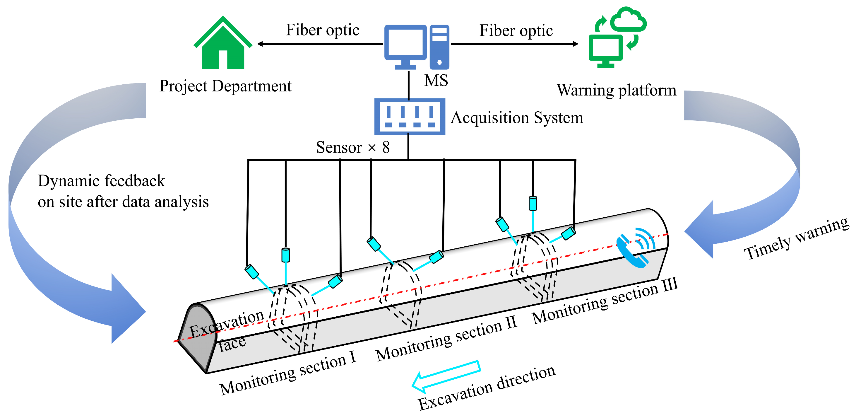
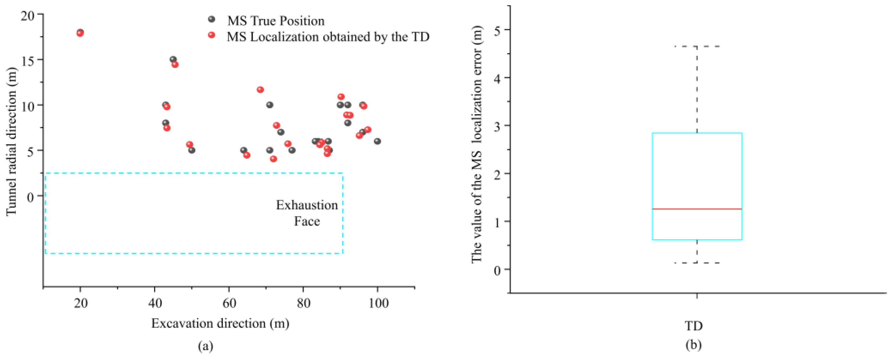
2.1. Real-Time Observation System

During tunnel excavation, the MS is deployed between the tunnel crown and the sidewalls with two or three monitoring surfaces for real-time microseismic monitoring. The MS equipment mainly includes microseismic sensors, data acquisition units, microseismic monitoring servers, and other supporting devices. The typical layout of the MS in the tunnels during the drilling and blasting method is shown in Figure 2. A set of acquisition equipment contains eight uniaxial sensors, typically covering an area of 40–120 m behind the tunnel face, which advances as the tunnel face progresses. The sensors monitor the information of active and passive seismic sources in real time and upload it through a fiber optic ring network to the project department and the early warning cloud for real-time data analysis and the timely release of warning information. We hope to master the current and future states of unfavorable geological bodies using blasting and rock fracture information monitored by the MS.

2.2. Inversion of the RMS Velocity Field Based on Microseismic Sources

2.2.1. Time–Distance Curve Equation in Cases of Nonlinear Seismic Sources

As previously discussed, our goal is to establish an RMS velocity field based on the propagation paths of passive seismic sources in an ideal medium without considering multiple waves. Following established research approaches, the RMS velocity field is constructed using a time–distance curve equation. This equation reflects the theoretical travel time of a primary reflection wave when it arrives, describing the paths of wave propagation in a homogeneous medium in accordance with the Fermat principle. For the horizontal interface illustrated in Figure 3a, the time–distance curve equation can be formulated as Equation (1),

$$\left\{\begin{array}{l}{t}^2\left(M_i\right)=4\left[{\left({\displaystyle \frac{h}{v_0}}\right)}^2+{\left({\displaystyle \frac{X_i}{2v_0}}\right)}^2\right]\\ t_0={\displaystyle \frac{2h_i}{v_0}}\end{array}\right.\Rightarrow t^2\left(M_i\right)={t_0}^2+{\left({\displaystyle \frac{X_i}{v_0}}\right)}^2$$

(1)

where the following is the case:

• t represents the first reflected wave travel time;
• v₀ represents the RMS velocity value in a homogeneous medium;
• X_i is the horizontal distance between the seismic source and the sensor;
• t₀ is self-excitation and self-collection time;
• h is the depth of the corresponding layer.

The RMS velocity field obtained during the inversion process can be converted into the laminar velocity field for stacking migration imaging using the Dix formula. For the faulted medium in the tunnel excavation direction, as shown in Figure 3b, we can derive the time-distance curve equation for the seismic sources in the tunnel observation system via the same approach, expressed as Equation (2), as follows:

$${t_i}^2\left(M_i\right)={\displaystyle \frac{{S_i}^2+{H_i}^2-2S_i{H}_i\cos \left(\alpha +{\alpha }^{\prime }\right)}{v_0^2}}$$

(2)

Figure 3. Schematic diagram of the seismic source propagation path without considering multiple waves: (a) vertical construction propagation path; (b) horizontal construction propagation path.

Figure 3. Schematic diagram of the seismic source propagation path without considering multiple waves: (a) vertical construction propagation path; (b) horizontal construction propagation path.

In the xy-plane, Si represents the distance between the sensor and the seismic source, calculated using the built-in positioning algorithm of the MS. H_i is the shortest distance from the seismic source to the fault interface, which is defined as half of the self-excitation and self-collection travel path, and α′ is the angle between the line connecting the seismic source and the sensor and the vertical direction, determined by Equation (3). α represents the angle between the fault interface and the tunnel axis. For discontinuous bodies nearly perpendicular to the tunnel axis, Equation (2) can be simplified to Equation (4), representing the conventional linear TSP forward geological prediction observation mode’s time–distance curve equation, as follows:

$${\alpha }^{\prime }=\arctan \left|{\displaystyle \frac{x_i-x_{sensor}}{{\mathrm{y}}_i-y_{sensor}}}\right|,{\alpha }^{\prime }\le 90°$$

(3)

$$t_i={\displaystyle \frac{S_i+2H_i}{v}}$$

(4)

For the self-excitation and self-collection travel path corresponding to each non-linear seismic source inside the tunnel, taking the travel path corresponding to the nearest source to the structural surface as an example, the travel path corresponding to the other sources can be expressed as in Equation (5a,b),

$$\begin{array}{l}{H}_i=2\left(H_1+\sin (\alpha -\beta )\sqrt{{\left(x_i-x_1\right)}^2+{\left(y_i-y_1\right)}^2}\right)y_i<y_1(a)\\ H_i=2\left(H_1+\sin (\alpha +\beta )\sqrt{{\left(x_i-x_1\right)}^2+{\left(y_i-y_1\right)}^2}\right)y_i>y_1(b)\end{array}$$

(5)

Here, β is the angle between the line connecting source M_i+1 and source M_i and the vertical axis direction in the xy-plane, which can be determined using Equation (6):

$$\beta =\arctan \left|{\displaystyle \frac{y_i-y_1}{x_i-x_1}}\right|,\beta \le 90°$$

(6)

By combining Equations (2) and (6), we obtain Equation (7a,b):

$$\begin{array}{c}{t}_i^2={\left({\displaystyle \frac{S_i}{v_{\mathrm{ori}}}}\right)}^2+{\displaystyle \frac{4{\left(H_1+\sin (\alpha -\beta )\sqrt{{\left(x_i-x_1\right)}^2+{\left(y_i-y_1\right)}^2}\right)}^2}{v^2}}-{\displaystyle \frac{2S_i\cos \left(\alpha +{\alpha }^{\prime }\right)2\left(h+\sin (\alpha -\beta )\sqrt{{\left(x_i-x_1\right)}^2+{\left(y_i-y_1\right)}^2}\right)}{v_{\mathrm{ori}}v}}\\ y_i\le y_1(a)\\ t_i^2={\left({\displaystyle \frac{S_i}{v_{\mathrm{ori}}}}\right)}^2+{\displaystyle \frac{4{\left(H_1+\sin (\alpha +\beta )\sqrt{{\left(x_i-x_1\right)}^2+{\left(y_i-y_1\right)}^2}\right)}^2}{v^2}}-{\displaystyle \frac{2S_i\cos \left(\alpha +{\alpha }^{\prime }\right)2\left(h+\sin (\alpha -\beta )\sqrt{{\left(x_i-x_1\right)}^2+{\left(y_i-y_1\right)}^2}\right)}{v_{\mathrm{ori}}v}}\\ y_i\ge y_1(b)\end{array}$$

(7)

Finally, this study establishes a nonlinear seismic source time–distance curve equation in an ideal layered medium. It is not difficult to see from Equation (7) that this travel time model is closely related to the establishment of the RMS velocity field.

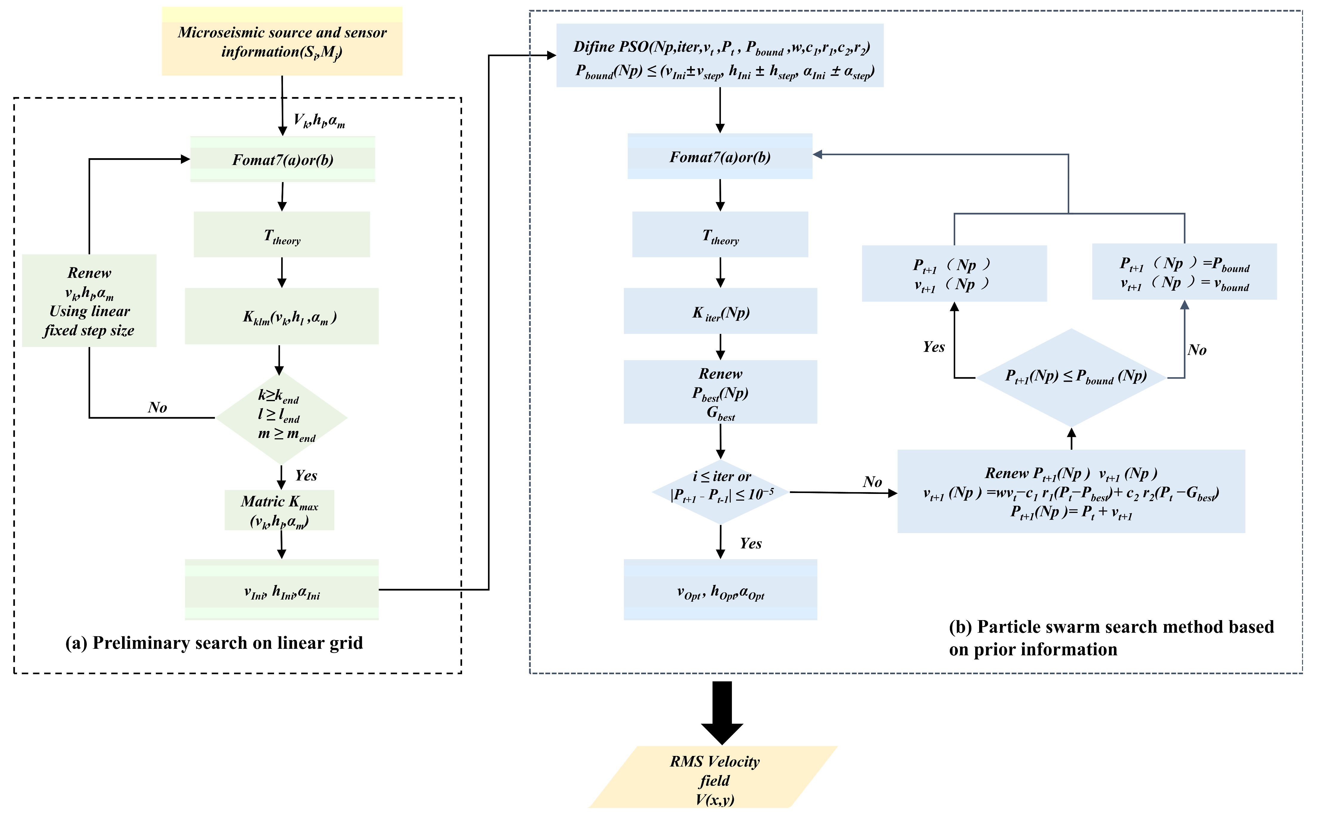
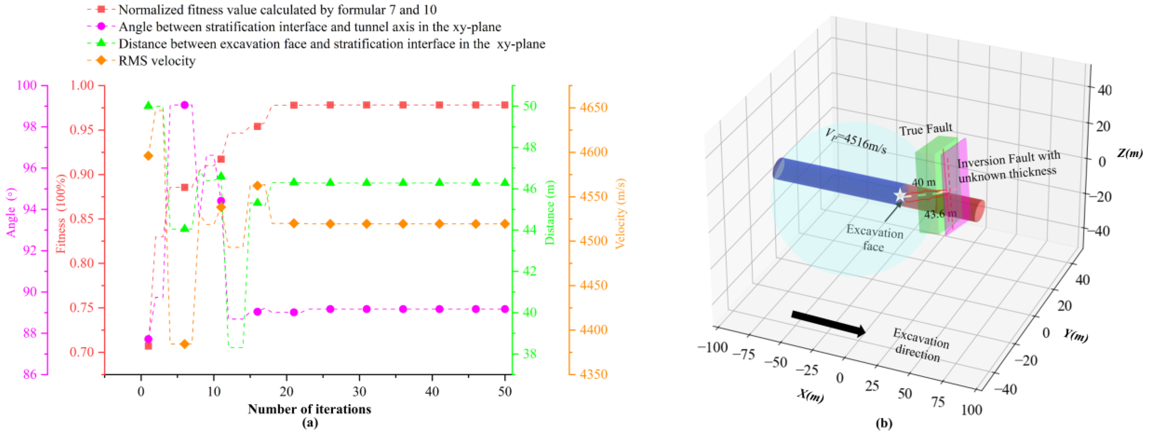
2.2.2. PSO Nonlinear Search Method for Establishing the RMS Velocity Field

After establishing Equation (7), the corresponding theoretical reflection wave travel time can be derived based on the given parameters. For microseismic sources that are disorganized, the absence of coherent axes complicates the direct observation of reflected wave arrival times, preventing the construction of a least squares solution between theoretical calculations and actual reflected wave arrival times. Consequently, the objective function is adapted to evaluate the similarity between the theoretical arrival times and the signals within the designated windows. The most widely used methods for evaluating similarity information are divided into stacking and similarity coefficient methods, as shown in Equation (8a–c) [25].

$$\begin{array}{c}E={\displaystyle \sum _{j=1}^M}{\left({\displaystyle \frac{1}{N}}{\displaystyle \sum _{i=1}^N}{f}_{i,j+r_i}\right)}^2\hspace{1em}\hspace{1em}\hspace{1em}\left(a\right)\\ S_c={\displaystyle \frac{{\displaystyle \sum _{j=1}^M}{\left({\displaystyle \sum _{i=1}^N}{f}_{i,j+r_i}\right)}^2}{N{\displaystyle \sum _{j=1}^M}{\displaystyle \sum _{i=1}^N}{f}_{i_s,j+r_i}^2}}\hspace{1em}\hspace{1em}\hspace{1em}\left(b\right)\\ corr={\displaystyle \frac{2}{N(N+1)}}{\displaystyle \sum _{i=1}^{N-1}}{\displaystyle \sum _{i^{\prime }>i}^N}{\displaystyle \sum _{j=0}^M}{\displaystyle \frac{f_{i,j+r_i}{f}_{i,j+r_i^{\prime }}}{\sqrt{{\displaystyle \sum _{j=0}^M}{f}_{i,j+r_i}^2{\displaystyle \sum _{j=0}^M}{f}_{i,j+r_i^{\prime }}^2}}}\hspace{0.17em}\left(c\right)\end{array}$$

(8)

In Equation (8), N denotes the number of traces within the selected window, M refers to the window size, and f represents the amplitude at each sampling point. These methods tend to be well-suited for systems featuring a single seismic source and multiple detectors. However, in an MS, there is a significant degree of anisotropy in both the relative signal-to-noise ratio (SNR) and amplitude spectrum among microseismic sources, which negatively affects the adaptability of these methods. Consequently, this study adopts an approach inspired by Chen [26] for calculating the SNR, and introduces an evaluation metric K that integrates both correlation and SNR to improve the applicability of these methods. The formulas for the SNR and K are provided in Equations (9) and (10), respectively.

$$SNR=10{\log }_{10}\left\{{\displaystyle \frac{{\sigma }^2\left[M_{\mathrm{windows}}\left(t\right)\right]-{\sigma }^2[n(t)]}{{\sigma }^2[n(t)]}}\right\}$$

(9)

$$\begin{array}{c}K={\displaystyle \frac{2}{N(N+1)}}{\displaystyle \sum _{i=1}^{N-1}\sum _{i^{\prime }>i}^N\sum _{j=0}^M}{\displaystyle \frac{f_{i,j+r_i}{f}_{i_i,j+r_i^{\prime }}\sqrt{\frac{SN{R}_{i}SN{R}_{i^{\prime }}}{SN{R}_{\max }^2}}}{\sqrt{{\displaystyle \sum _{j=0}^M}{f}_{i,j+r_i}^2{\displaystyle \sum _{j=0}^M}{f}_{i_i,j+{r_i}^{\prime }}^2}}}\\ ={\displaystyle \frac{2}{N(N+1)}}{\displaystyle \sum _{i=1}^{N-1}\sum _{i^{\prime }>i}^N}{\displaystyle \frac{R_{i{i}^{\prime }}(0,H,v,\alpha )S\left(i,i^{\prime }\right)}{\sqrt{R_{ii}(0,H,v,\alpha )S\left(i,i^{\prime }\right)}}}\end{array}$$

(10)

In Equation (9), M_windows represents the theoretical arrival time data. In Equation (10), R signifies the non-normalized cross-correlation values obtained from seismic data along the propagation trajectory with zero-time delay, and S stands for the normalized signal-to-noise ratio weight of adjacent traces. The final inversion result corresponds to the parameters for which the computed comprehensive evaluation index K is maximized.

It is important to note that conventional methods for analyzing a travel-time curve RMS velocity field have often relied on simple grid searches. However, optimization algorithms can be limited in multi-extremum inversions. In this study, we considered the advantages of PSO in updating search directions nonlinearly. We adopted a PSO-based parameter inversion approach with passive seismic information that incorporates prior information from grid searches. By determining the optimal values of K from theoretical inversions, we established the inversion process for establishing the RMS velocity field, as depicted in Figure 4.

The calculation steps for the proposed RMS velocity field based on PSO are as follows:

• Step 1—Select signals with high signal-to-noise ratios from the nonlinear seismic source parameters (xi, yi, t0i) computed in Section 2.1 based on the MS. These signals are reassembled into profiles to serve as the inputs for inversion;
• Step 2—Implement a linear search strategy with specifically set intervals (v_step, h_step, α_step) for the grid search, taking into account the findings from prior geological surveys during the initial phase of the inversion process;
• Step 3—Using the nonlinear seismic source parameters and sensor coordinates from Step 1, calculate the theoretical arrival times T_theory of reflected waves based on Equation (7) under the designated parameters (v_t, h_l, α_m);
• Step 4—Window the signals based on the theoretical arrival times T_theory using a Hamming window to obtain the windowed data S_window;
• Step 5—Using the proposed correlation function K from Equation (10), calculate the comprehensive evaluation index and generate the correlation matrix K (v_t, h_l, α_m);
• Step 6—From Step 5, choose the parameters corresponding to the maximum value Corr(K) in the correlation matrix as the starting input values for the PSO algorithm. Define the particle search range and initialize the particle parameters, which include the number of particles Np, current flight speed v_t, position P_t, position P_boundary, individual best values P_best, group best values g_best, and some common control parameters for PSO algorithms (w, c₁, r₁, c₂, r₂);
• Step 7—Repeat Steps 3–5, update the parameters, and end the loop when conditions are met. Output the current optimal values and corresponding parameters, which will be used to establish the initial RMS velocity field model (v_{opt, hopt}, α_opt).

2.3. Adjoint-State Full-Waveform Inversion Based on the RMS Velocity Model and Blasting Seismic Sources

It is worth noting that the method described in Section 2.2 directly fits fault structures or the RMS velocity field, such as y = f(x, α, v), using passive seismic sources observed by the MS. However, for a single structure such as the one depicted in Figure 3b, due to the difference between the microseismic signals from different sources, it is difficult to directly apply adjoint-state full-waveform inversion to obtain the heterogenous P-wave velocity field for fault detection because of the lack of information on the time of earthquake occurrence. To address this limitation, this study integrates information from the known blasting seismic sources, with the RMS velocity field optimized from passive seismic sources to enable the updating of the velocity field to approach the real wave field, thus achieving precise imaging of the target area [27,28,29].

By replacing the conventional least-squares objective function with the formula specified in Equation (11), and integrating features of RTM theory, this study utilizes a cross-correlation objective function to invert the velocity field in Equation (12). This function effectively mitigates the impact of variations in active source quality due to factors such as borehole conditions, explosive charges, and the coupling between the explosives and the surrounding rock, as well as the unevenness in micro-seismic amplitude information, thereby significantly enhancing the robustness of the inversion results against noise.

$$J_1(v)={\displaystyle \frac{1}{2}}\sum _{N_{\mathrm{s}},N_{\mathrm{r}}}{{\displaystyle \int }}_t{\left[d_{\mathrm{syn}}-d_{\mathrm{obs}}\right]}^2\mathrm{d}t$$

(11)

$$J_2(v)=-\sum _{N_{\mathrm{s}},N_{\mathrm{r}}}{\displaystyle \frac{{{\displaystyle \int }}_t\left(d_{\mathrm{syn}}{d}_{\mathrm{obs}}\right)\mathrm{d}t}{\sqrt{{{\displaystyle \int }}_t{d}_{\mathrm{syn}}^2\mathrm{d}t}\sqrt{{{\displaystyle \int }}_t{d}_{\mathrm{obs}}^2\mathrm{d}t}}}$$

(12)

Here, N_s and N_r represent the numbers of microseismic sensors and seismic sources, respectively; d_syn represents the forward data under the current model; and d_obs represents the blasting seismic data received by the microseismic sensors. For the objective function in Equation (13), we typically use methods such as the conjugate gradient or the adjoint-state method. In this study, we mainly employ the adjoint-state method to compute the gradient of the objective function. The gradient calculation method is shown in Equation (14):

$${\displaystyle \frac{\mathsf{\partial }J(v)}{\mathsf{\partial }v}}=\sum _{N_{\mathrm{s}},N_{\mathrm{r}}}{{\displaystyle \int }}_t{\displaystyle \frac{\mathsf{\partial }{d}_{\mathrm{cal}}}{\mathsf{\partial }v}}\cdot \chi \mathrm{d}t$$

(13)

$$\chi ={\displaystyle \frac{{{\displaystyle \int }}_t\left(d_{\mathrm{syn}}{d}_{\mathrm{obs}}\right)\mathrm{d}t\cdot d_{\mathrm{syn}}}{{\sqrt{{\displaystyle \underset{t}{\int }{d}_{\mathrm{syn}}^{2}dt}}}^3\sqrt{{{\displaystyle \int }}_t{d}_{\mathrm{obs}}^2\mathrm{d}t}}}-{\displaystyle \frac{d_{\mathrm{obs}}}{\sqrt{{{\displaystyle \int }}_t{d}_{\mathrm{syn}}^2\mathrm{d}t}\sqrt{{{\displaystyle \int }}_t{d}_{\mathrm{obs}}^2\mathrm{d}t}}}$$

(14)

Here, χ represents the adjoint source, which is the residual wavefield between the observed wavefield and the simulated wavefield based on RTM theory; thus, the velocity gradient formula in the time domain can be simplified to Equation (15),

$${\displaystyle \frac{\mathsf{\partial }J(v)}{\mathsf{\partial }v}}={\displaystyle \frac{2}{v^3}}\sum _{N_{\mathrm{s}},N_{\mathrm{r}}}{{\displaystyle \int }}_t{\displaystyle \frac{{\mathsf{\partial }}^2{P}_{\mathrm{f}}}{\mathsf{\partial }{t}^2}}\cdot P_{\mathrm{r}}^{\chi }\mathrm{d}t$$

(15)

where P_r^χ is the reverse-time wavefield of the adjoint source. Through the established gradient iteration formula, we can establish the final velocity field model. Its gradient iteration formula and gradient update step calculation formula can be expressed as Equations (16) and (17),

$${\displaystyle \frac{\mathsf{\partial }J(v+1)}{\mathsf{\partial }v}}={\displaystyle \frac{\mathsf{\partial }J(v)}{\mathsf{\partial }v}}-{\alpha }_k{\displaystyle \frac{\mathsf{\partial }J(v)}{\mathsf{\partial }v}}$$

(16)

$${\alpha }_k=max\left(0,{\alpha }_1,{\alpha }_2\right)\left\{\begin{array}{l}{\alpha }_1={\displaystyle \frac{{\displaystyle \sum _{N_{\mathrm{s}},N_{\mathrm{r}}}(\frac{\mathsf{\partial }J\left(v+1\right)}{\mathsf{\partial }v})\cdot {(\frac{\mathsf{\partial }J\left(v+1\right)}{\mathsf{\partial }v})}^T}}{{\displaystyle \sum _{N_{\mathrm{s}},N_{\mathrm{r}}}{V}_{k+1}^T\cdot \left(\frac{\mathsf{\partial }J\left(v+1\right)}{\mathsf{\partial }v}-\frac{\mathsf{\partial }J}{\mathsf{\partial }v}\right)}}}\\ {\alpha }_2={\displaystyle \frac{{\displaystyle \sum _{N_{\mathrm{s}},N_{\mathrm{r}}}{(\frac{\mathsf{\partial }J\left(v+1\right)}{\mathsf{\partial }v}-\frac{\mathsf{\partial }J}{\mathsf{\partial }v})}^T\cdot (\frac{\mathsf{\partial }J\left(v+1\right)}{\mathsf{\partial }v}-\frac{\mathsf{\partial }J}{\mathsf{\partial }v})}}{{\displaystyle \sum _{N_{\mathrm{s}},N_{\mathrm{r}}}{V}_{k+1}^T\cdot (\frac{\mathsf{\partial }J\left(v+1\right)}{\mathsf{\partial }v}-\frac{\mathsf{\partial }J}{\mathsf{\partial }v})}}}\end{array}\right.$$

(17)

In summary, by combining Section 2.1, Section 2.2 and Section 2.3, this study establishes a velocity inversion method for detecting faults in tunnel construction using both rock fracture passive seismic sources and blasting sources.

3. Numerical Validation

We used numerical simulations of actual deep tunnel models to characterize the propagation properties of waves within the tunnels. During the simulation process, we will consider the influence of the Excavation Damaged Zone (EDZ). We use seismic data from rock fractures and blasting to invert the velocity model. Finally, we compare the inverted results with the real velocity model to verify the accuracy of the proposed joint active–passive seismic source method for detecting faults based on the velocity field in tunnels.

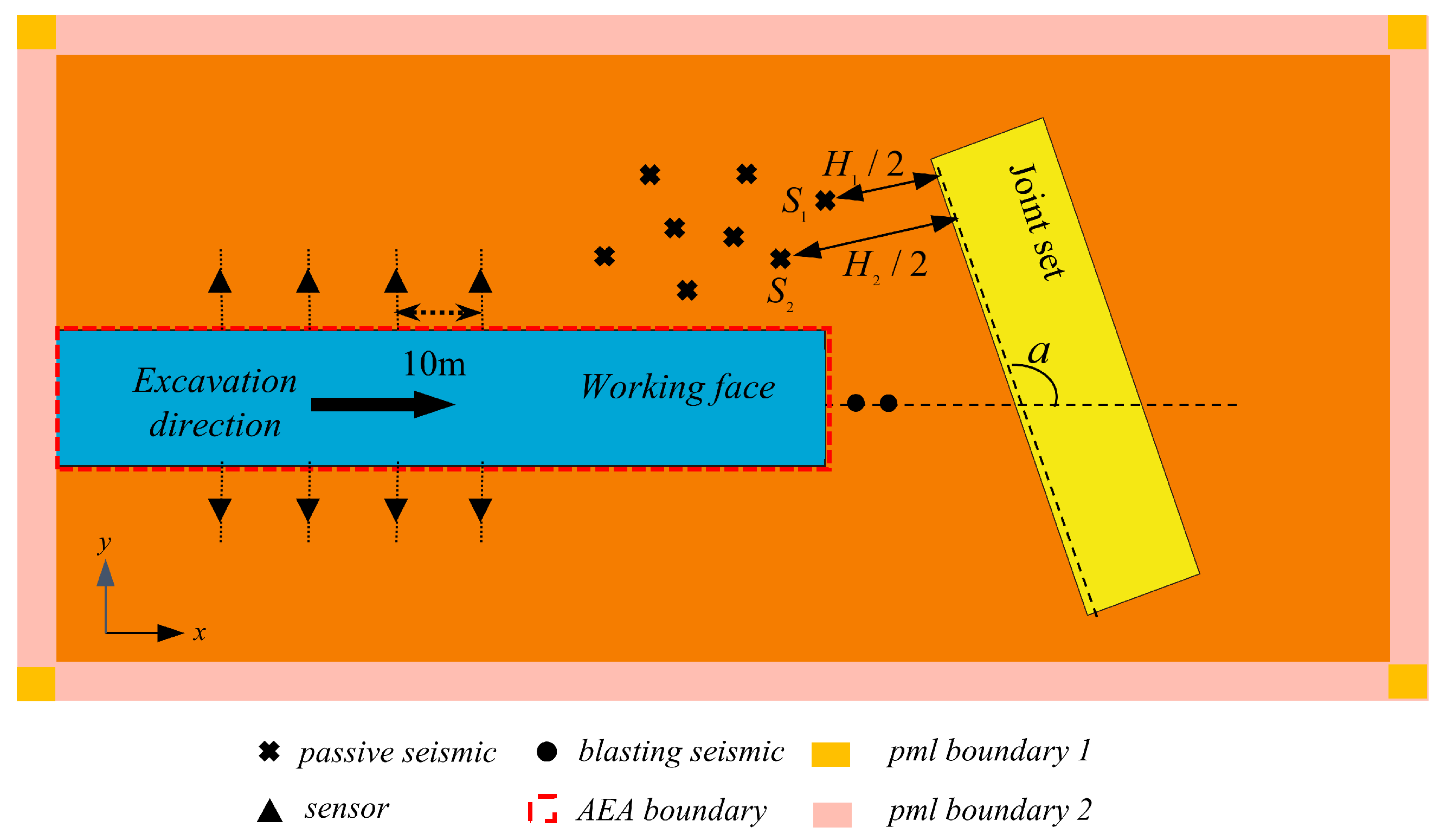
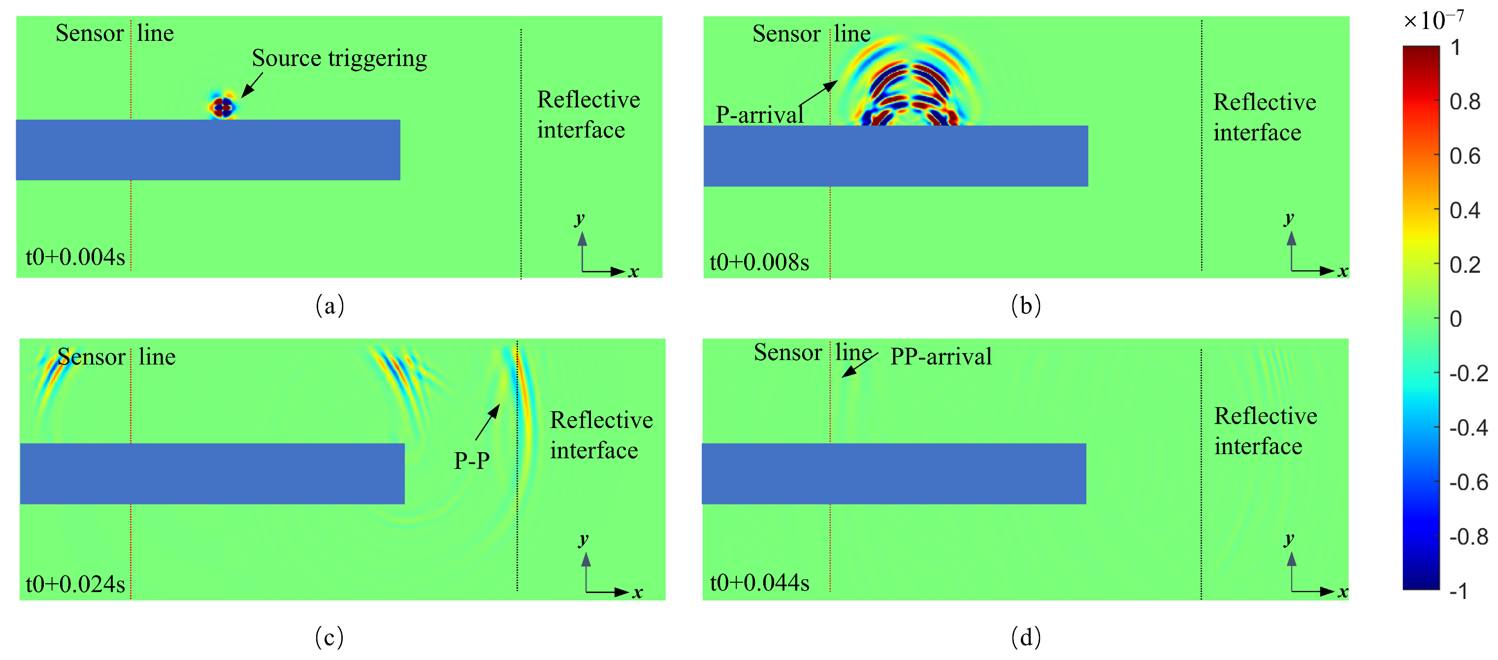
3.1. Numerical Modeling and MS Simulation

We first establish a common tunnel microseismic observation system in the xy-plane. It simulates multiple random fracture seismic sources within the monitoring range based on the two-dimensional time-domain elastic equations. Furthermore, convolutional perfectly matched layer (CPML) boundaries were defined at the calculation domain’s boundaries [30], and an absorbing edge boundary (AEA) was defined in the Excavation Damaged Zone (EDZ) region to better reflect the wave field’s propagation characteristics [31]. The elastic wave equation used in this paper is shown in Equation (18) [32], and the source wavelet employed was a Ricker wavelet with a dominant frequency f_m of 200 Hz, as shown in Figure 5.

$$\begin{array}{c}{\displaystyle \frac{\mathsf{\partial }{v}_x}{\mathsf{\partial }t}}={\displaystyle \frac{1}{\rho }}\left({\displaystyle \frac{\mathsf{\partial }{\tau }_{xx}}{\mathsf{\partial }x}}+{\displaystyle \frac{\mathsf{\partial }{\tau }_{xy}}{\mathsf{\partial }y}}\right)\\ {\displaystyle \frac{\mathsf{\partial }{v}_y}{\mathsf{\partial }t}}={\displaystyle \frac{1}{\rho }}\left({\displaystyle \frac{\mathsf{\partial }{\tau }_{xy}}{\mathsf{\partial }x}}+{\displaystyle \frac{\mathsf{\partial }{\tau }_{yy}}{\mathsf{\partial }y}}\right)\\ {\displaystyle \frac{\mathsf{\partial }{\tau }_{xx}}{\mathsf{\partial }t}}=(\lambda +2G){\displaystyle \frac{\mathsf{\partial }{v}_x}{\mathsf{\partial }x}}+\lambda {\displaystyle \frac{\mathsf{\partial }{v}_y}{\mathsf{\partial }y}}\\ {\displaystyle \frac{\mathsf{\partial }{\tau }_{yy}}{\mathsf{\partial }t}}=(\lambda +2G){\displaystyle \frac{\mathsf{\partial }{v}_y}{\mathsf{\partial }y}}+\lambda {\displaystyle \frac{\mathsf{\partial }{v}_x}{\mathsf{\partial }x}}\\ {\displaystyle \frac{\mathsf{\partial }{\tau }_{xy}}{\mathsf{\partial }t}}=G\left({\displaystyle \frac{\mathsf{\partial }{v}_x}{\mathsf{\partial }y}}+{\displaystyle \frac{\mathsf{\partial }{v}_y}{\mathsf{\partial }x}}\right)\end{array}$$

(18)

As shown in Figure 6, the model measured 150 m in length × 50 m in width, with a 0.25 m spatial interval in both the x- and y-directions. The designated tunnel area, shaped as a rectangle, spanned from the starting point at (0, 20) to the endpoint at (90, 30). For this simulation, the MS was positioned on both sides of the tunnel’s sidewall, comprising eight sensors with coordinates J1 (30, 17), J2 (40, 17), J3 (50, 17), J4 (60, 17), J5 (30, 33), J6 (40, 33), J7 (50, 33), and J8 (60, 33). The microseismic source locations ranged between the x-coordinates of 40 and 100 and the y-coordinates of 5 and 20. The background properties, consisting of the surrounding rock’s P-wave and S-wave velocities and density, were 4500 m/s, 2600 m/s, and 2 g/cm³, respectively. Near the fault zone, the medium properties were a P-wave velocity of 3500 m/s, an S-wave velocity of 2000 m/s, and a density of 1 g/cm³. The sampling rate was set at 2 × 10⁻⁵ s, with a total simulation time of 0.06 s.

From the wavefield snapshots of the seismic source propagation process at different times based on the MS shown in Figure 7a–d, it was observed that the energy of the reflected waves in the theoretical reflection zone was relatively weak. In this study, noise was added, and constant Q compensation was applied to the forward-modeled data, reflecting the unique characteristics of the microseismic sources. The noise addition function is shown in Equation (19), where i and j represent the number of sampling points and the number of seismic traces, and the waveforms from different seismic sources recorded by the same sensor, before and after the addition of noise and the application of Q compensation, are shown in Figure 8a,b.

$${\mathrm{d}}_{i,j}={\mathrm{d}}_{i,j}+{\displaystyle \frac{\frac{1}{N}{\displaystyle \sum _{i=1}^N{d}_{i,j}^2}}{{10}^{\frac{SNR}{10}}}}$$

(19)

In Section 3.2, we applied the TD (Time Difference) localization method to the passive source observation data. In this method, we assumed an unknown velocity field and performed localization using only five sensors based on the MS [33]. The resulting localization data were then reorganized into profiles to serve as input models for the method described in Section 2.1.

Table 1. Source location and localization results based on TD.

Number	True Position	Source Location	Error in the y-Direction	Error in the x-Direction	Localization Error
	(m)	(m)	(m)	(m)	(m)
1	(5, 77)	(5.72, 75.88)	−0.72	−1.02	1.25
2	(7, 74)	(7.75, 72.81)	0.75	−1.21	1.42
3	(10, 43)	(9.78, 43.33)	−1.22	0.33	1.26
4	(10, 96)	(9.86, 96.31)	−0.14	0.31	0.34
5	(6, 84)	(4.64, 86.51)	−1.36	2.51	2.85
6	(6, 85)	(5.87, 85.01)	−0.13	0.01	0.13
7	(8, 43)	(7.45, 43.30)	−0.55	0.30	0.63
8	(8, 92)	(6.62, 95.12)	−1.38	3.12	3.41
9	(7, 96)	(8.89, 91.75)	1.89	−4.25	4.65
10	(6, 100)	(7.26, 97.38)	1.266	−2.62	2.91
11	(10, 92)	(10.90, 90.19)	0.9	−1.81	2.02
12	(5, 87)	(5.21, 86.49)	0.21	−0.51	0.55
13	(5, 71)	(4.05, 72.03)	−0.95	1.03	1.40
14	(5, 50)	(5.65, 49.41)	0.65	−0.59	0.88
15	(5, 64)	(4.45, 64.84)	−0.55	0.84	1.00
16	(10, 90)	(8.86, 92.59)	−1.14	2.59	2.83
17	(6, 85)	(5.61, 85.45)	−0.39	0.45	0.60
18	(15, 45)	(14.43, 45.53)	−0.57	0.53	0.78
19	(10, 71)	(11.66, 68.46)	1.66	−2.54	3.03
20	(18, 20)	(17.85, 19.90)	−0.15	−0.1	0.18

shows the microseismic source localization results, while Figure 9 displays the distribution maps before and after localization, along with the localization error boxplot. From the perspective of the positioning results, the maximum error before and after seismic source localization was around 5 m, with an average error of about 1.5 m. Considering the assumed distribution of 20 rock fracture seismic sources, they exhibited a strong nonlinearity with respect to the sensors. It is worth noting that in Figure 8, it is not difficult to see that the nonlinearity of heterogeneous seismic sources makes it difficult to pick up the events directly. This characteristic facilitates the validation of the proposed nonlinear travel-time curve model in this paper. We solved this problem through the method proposed in Section 2.2. However, due to the nonsensitivity of the microseismic positioning process to the time of detonation, and the high accuracy requirement of full waveform inversion for the time of detonation, we chose a blasting source that could relatively effectively control the detonation time.

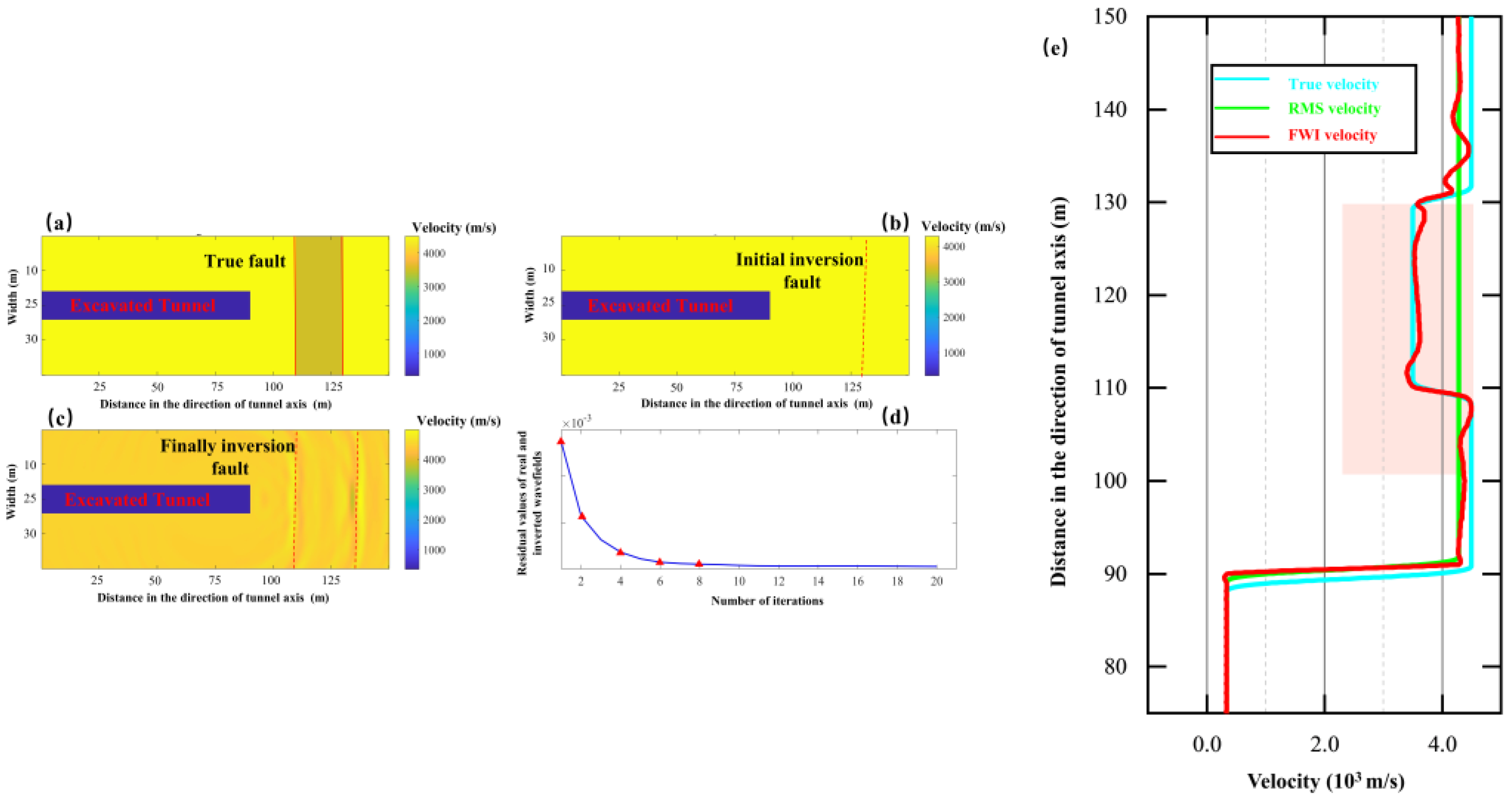
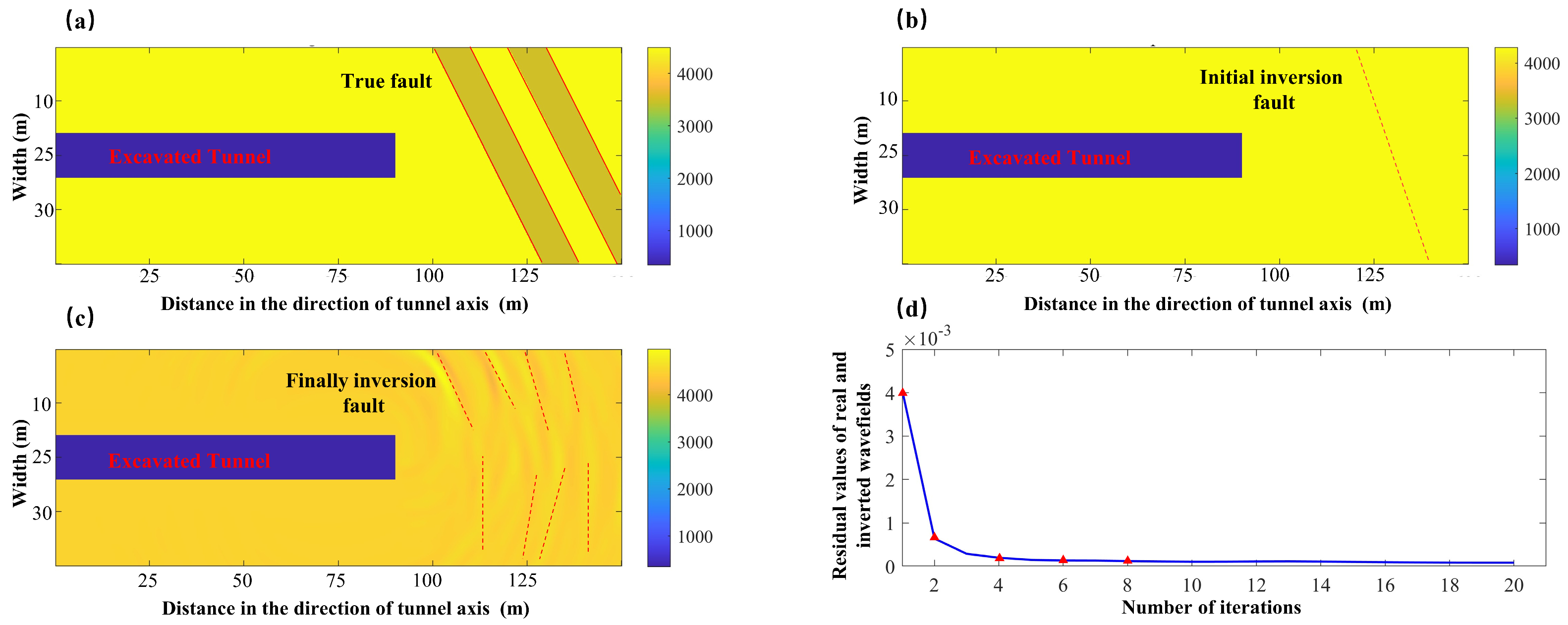
3.2. Validation and Performance Analysis of Inversion Methods

Based on the preliminary passive source localization information and observation data, we applied the method proposed in Section 2.2.1 to conduct a linear grid search for the RMS velocity field in the simulated area. The three-dimensional results of the grid search in terms of the RMS velocity field are shown in Figure 10. In the image, the red area represents the input search range of the PSO described in Section 2.2.2, and the search range for the three parameters is v from 4000 to 5000 m/s, with an α of 80–120 degrees and an h of 20–50 m. Subsequently, based on the search range of the RMS velocity field, we used the PSO nonlinear search method proposed in Section 2.2.2 to invert the final RMS velocity field as the initial velocity field of the monitoring area. We calculated the velocity parameter based on Formulas (7)–(10). The inversion results of the final RMS velocity field and inversion fault model are shown in Figure 11.

From the final results, we can see that based on the method proposed in Section 2.2, there was a certain deviation in the RMS velocity field. For example, the relative position between the current working face and the fault should be 20–40 m, while the final inversion value was around 44 m. This was because, using the method in Section 2.2, we only approximated the theoretical propagation path of the seismic source using the reflection wave ray-tracing method, and the location of the source was also inaccurate. This method provided us with initial fault information (more precisely, the location information of the fault, not the thickness information) and solved the cycle-skipping phenomenon in FWI. As mentioned earlier, for the blasting source of the excavation face, the actual time and location of the source can be approximately recorded. To obtain more accurate velocity field information, it is necessary to perform full waveform gradient correction based on this RMS velocity field.

Subsequently, the RMS velocity field inverted using the current PSO was used as the initial velocity model for FWI. Given the conditions of the inverted velocity field model and the need for efficient inversion, we utilized the recorded signals from five blasting active seismic sources within our observation system. These signals served as our observed sources for full-waveform inversion, all under the same boundary conditions. Specific details regarding the locations of these blasting sources are provided in

Table 2. Information of blasting seismic sources.

Blasting Number	Position x (m)	Position y (m)
1	93	25
2	96	25
3	99	25
4	102	25
5	105	25

.

The results of FWI are shown in Figure 12a–d. From the results, it can be seen that, based on the RMS velocity field established in Section 2 and the FWI method for inverting the velocity fields, even with some offset noise, we can still clearly see the abnormal velocity values at the fault boundary. To further assess the method’s accuracy, we extracted the wave speed distribution along the tunnel axis shown in Figure 12e. For instance, up to a distance of 90 m and within the tunnel width range, both the true and input model wave speeds were set at 340 m/s. Our focus lay in comparing the velocity discrepancies highlighted in the diagram. Although there was a slight overestimation of velocity at the fault boundary, the difference in the inverted fault thickness from the true value was minimal. This discrepancy did not hinder our ability to accurately determine the fault’s real shape and position. Based on the results, when the quality of blasting data is dependable and both the location and seismic moment are determined, the method proposed in this paper enables the effective inversion of information pertaining to regular linear faults.

To further validate the adaptability of this method, we created additional typical cases based on the previous simulation conditions, including single-layer and double-layer structures with a 60° dip angle. The final results of the full waveform inversion are shown in Figure 13, Figure 14 and Figure 15. From these results, it is evident that the proposed joint inversion method for the blasting and passive seismic sources exhibits strong adaptability to velocity structures with “linear” characteristics, often converging to the structural features in around 10 iterations. However, due to the narrow observation aperture of the tunnel and the large inclination angle of the anomalous body, it is difficult for the detector to receive effective reflection signals from the side of the anomalous body far from the palm surface. Therefore, the imaging effect of the fault boundary far from the palm face is not good. Furthermore, the adaptability of the tunnel observation system to cave structures is limited. Due to the system’s limitations and uneven illumination, it is relatively easy to consider the arc-shaped boundary of the karst cave as a layered boundary.

Furthermore, we summarized the error results of the fault detection method proposed in this article under different working conditions during the passive and active source detection stages, as shown in

Table 3. Summary of inversion errors at different stages under different operating conditions.

Case	Stage	Fault Position in X-Axis (m)	Fault Thickness (m)
Rectangular fault model	1	14	×
	2	2	5
Single-dip structural fault model	1	9	×
	2	4	1
Double-dip structural fault mode	1	9(7)	×
	2	2.3	2.1
Circular karst cave model	1	13	×
	2	1	5

(× represents that the corresponding result cannot be calculated at this stage).

. We defined the process of fault inversion in this article as taking place over two stages—passive and active source inversion— and we used the boundary and thickness of the leftmost interface of the anomalous velocity body as references for inversion errors. The results from the different cases indicate that during the passive source exploration phase, the initial position information of the velocity structure could be inferred. However, due to its resemblance to a single straight-line fitting process, errors were larger. Building on this foundation, the active source exploration phase primarily addressed the issue of fault thickness information.

4. Discussion

In this study, various typical numerical simulation scenarios demonstrated that the proposed joint inversion method for active and passive seismic sources can theoretically address real-time geophysical exploration challenges in tunnels, particularly for structures with regular linear features. The velocity model is essential for the fault disaster warning work of the MS. However, certain aspects of the proposed inversion method require further discussion.

Firstly, the method proposed in this article to invert the RMS velocity using micro-seismic events is mainly used for deep-buried hard rock tunnels, and it is difficult to consider the influence of the EDZ region in establishing the travel-time curve model of the RMS velocity field. Additionally, the method of picking up the arrival time of reflected waves based on the similarity principle can also cause certain errors. Although ray-tracing methods can consider the influence of the EDZ region, they are primarily used to calculate the travel time of direct waves, mainly updating the velocity model, where the ray path density is high [34,35]. Accurately picking up the arrival time of reflected waves is crucial for the establishment of the velocity model. The overlap of reflected P-waves and S-waves in actual signals poses a challenge to picking up the arrival time of reflected waves. In further research, we can explore the identification of the arrival time of reflected waves based on the phase difference to establish a more accurate velocity model.

Additionally, in the numerical simulation process, the origin time of the seismic source signal is known, but in practical scenarios, recording the initiation time of the detonation signal from surface blasting is a topic for further discussion. We may need to use ray tracing to approximate the time of seismic source occurrence by using the RMS velocity field in reverse, or a trigger MS instrument will be required to directly record the t₀ blasting source under complex geological conditions, which can completely remove the error in the estimated t₀.

Finally, there is no noise interference between blasting source signals during adjoint-state full-waveform inversion, whereas actual blasting signals are often multi-segment millisecond-delayed mixed signals. Industrial testing is needed to control the appropriate initiation intervals and separate the initial segment of the blasting signal. For example, we can try to control the interval between the second and the first blasting signals to achieve this goal.

5. Conclusions

This paper introduced a heterogenous P-wave velocity inversion method for fault detection in deeply buried hard rock tunnels using active–passive seismic sources. A reflection wave ray-tracing method based on the time–distance curve model and PSO optimization method was proposed to establish an RMS velocity field based on the distribution and amplitude characteristics of heterogeneous micro seismic sources. When establishing the RMS velocity field, the diffraction effects of passive seismic sources within the tunnel void are generally not accounted for. If the seismic source is limited to surface blasting, this could result in a substantial amplification of the error.

Additionally, based on the RMS velocity field and blasting seismic source information, an adjoint-state full-waveform inversion was conducted to renew the heterogenous P-wave velocity model for fault detection. In the scenario where there were multiple types of abnormal structures, it was shown that coupling the microseismic signals with the excavation blasting signals of the palm surface monitored by MS can detect abnormal structures inside the tunnel. The errors observed in the inversion results suggest that the proposed method exhibits a high sensitivity to the velocity interface (faults).

However, due to the limitations of model assumptions and observation systems, there remain certain errors in the inversion results under nonlinear special conditions such as karst caves. Nevertheless, for MS systems, we can continuously utilize this seismic source information to perform real-time updates and corrections to the inversion results during tunnel excavation. Our ultimate goal is to provide early warnings of potential fault-slip disasters and the healthy control of geotechnical engineering by combining reverse-engineered fault information with newly generated microseismic events.

References

1. Cai, M.; Kaiser, P.K.; Martin, C.D. Quantification of Rock Mass Damage in Underground Excavations from Microseismic Event Monitoring. Int. J. Rock Mech. Min. Sci. 2001, 38, 1135–1145. [Google Scholar] [CrossRef]
2. Dai, F.; Li, B.; Xu, N.; Meng, G.; Wu, J.; Fan, Y. Microseismic Monitoring of the Left Bank Slope at the Baihetan Hydropower Station, China. Rock Mech. Rock Eng. 2017, 50, 225–232. [Google Scholar] [CrossRef]
3. Jiang, Q.; Yang, B.; Yan, F.; Xu, D.; Feng, G.; Li, S. Morphological Features and Fractography Analysis for in Situ Spalling in the China Jinping Underground Laboratory with a 2400 m Burial Depth. Tunn. Undergr. Space Technol. 2021, 118, 104194. [Google Scholar] [CrossRef]
4. You, R.-Z.; Yi, T.-H.; Ren, L.; Li, H.-N. Equivalent Estimation Method (EEM) for Quasi-Distributed Bridge-Deflection Measurement Using Only Strain Data. Measurement 2023, 221, 113492. [Google Scholar] [CrossRef]
5. You, R.-Z.; Yi, T.-H.; Ren, L.; Li, H.-N. Distributed Bending Stiffness Estimation of Bridges Using Adaptive Inverse Unit Load Method. Eng. Struct. 2023, 297, 116981. [Google Scholar] [CrossRef]
6. Cook, N.G.W. Seismicity Associated with Mining. Eng. Geol. 1976, 10, 99–122. [Google Scholar] [CrossRef]
7. Wamriew, D.; Dorhjie, D.B.; Bogoedov, D.; Pevzner, R.; Maltsev, E.; Charara, M.; Pissarenko, D.; Koroteev, D. Microseismic Monitoring and Analysis Using Cutting-Edge Technology: A Key Enabler for Reservoir Characterization. Remote Sens. 2022, 14, 3417. [Google Scholar] [CrossRef]
8. Chen, X.; Li, W.; Yan, X. Analysis on Rock Burst Danger when Fully-Mechanized Caving Coal Face Passed Fault with Deep Mining. Saf. Sci. 2012, 50, 645–648. [Google Scholar] [CrossRef]
9. Zhang, W.; Feng, X.-T.; Yao, Z.-B.; Hu, L.; Xiao, Y.-X.; Feng, G.-L.; Niu, W.-J.; Zhang, Y. Development and Occurrence Mechanisms of Fault-Slip Rockburst in a Deep Tunnel Excavated by Drilling and Blasting: A Case Study. Rock Mech. Rock Eng. 2022, 55, 5599–5618. [Google Scholar] [CrossRef]
10. BABEL Working Group Evidence for Early Proterozoic Plate Tectonics from Seismic Reflection Profiles in the Baltic Shield. Nature 1990, 348, 34–38. [CrossRef]
11. Alimoradi, A.; Moradzadeh, A.; Naderi, R.; Salehi, M.Z.; Etemadi, A. Prediction of Geological Hazardous Zones in Front of a Tunnel Face Using TSP-203 and Artificial Neural Networks. Tunn. Undergr. Space Technol. 2008, 23, 711–717. [Google Scholar] [CrossRef]
12. Claerbout, J.F. Toward a Unified Theory of Reflector Mapping. Geophysics 1971, 36, 467–481. [Google Scholar] [CrossRef]
13. French, W.S. Computer Migration of Oblique Seismic Reflection Profiles. Geophysics 1975, 40, 961–980. [Google Scholar] [CrossRef]
14. McMechan, G.A. Migration by Extrapolation of Time-Dependent Boundary Values. Geophys. Prospect. 1983, 31, 413–420. [Google Scholar] [CrossRef]
15. Dai, S.; Ma, C. Application of TSP Tunnel Geological Prediction for Case Study. In Mechatronics and Intelligent Materials II, Pts 1–6; Chen, R., Sung, W.P., Eds.; Trans Tech Publications Ltd.: Stafa-Zurich, Switzerland, 2012; Volume 490–495, pp. 1816–1820. [Google Scholar]
16. Yokota, Y.; Yamamoto, T.; Shirasagi, S.; Koizumi, Y.; Descour, J.; Kohlhaas, M. Evaluation of Geological Conditions Ahead of TBM Tunnel Using Wireless Seismic Reflector Tracing System. Tunn. Undergr. Space Technol. 2016, 57, 85–90. [Google Scholar] [CrossRef]
17. Li, S.; Liu, B.; Xu, X.; Nie, L.; Liu, Z.; Song, J.; Sun, H.; Chen, L.; Fan, K. An Overview of Ahead Geological Prospecting in Tunneling. Tunn. Undergr. Space Technol. 2017, 63, 69–94. [Google Scholar] [CrossRef]
18. Xu, X.; Zhang, P.; Guo, X.; Liu, B.; Chen, L.; Zhang, Q.; Nie, L.; Zhang, Y. A Case Study of Seismic Forward Prospecting Based on the Tunnel Seismic While Drilling and Active Seismic Methods. Bull. Eng. Geol. Environ. 2021, 80, 3553–3567. [Google Scholar] [CrossRef]
19. Shapiro, N.M.; Campillo, M. Emergence of Broadband Rayleigh Waves from Correlations of the Ambient Seismic Noise. Geophys. Res. Lett. 2004, 31. [Google Scholar] [CrossRef]
20. Hou, S.; Liu, Y.; Yang, Q. Real-Time Prediction of Rock Mass Classification Based on TBM Operation Big Data and Stacking Technique of Ensemble Learning. J. Rock Mech. Geotech. Eng. 2022, 14, 123–143. [Google Scholar] [CrossRef]
21. Nilot, E.A.; Fang, G.; Elita Li, Y.; Tan, Y.Z.; Cheng, A. Real-Time Tunneling Risk Forecasting Using Vibrations from the Working TBM. Tunn. Undergr. Space Technol. 2023, 139, 105213. [Google Scholar] [CrossRef]
22. Wang, S.; Han, L.; Gong, X.; Zhang, S.; Huang, X.; Zhang, P. MCMC Method of Inverse Problems Using a Neural Network—Application in GPR Crosshole Full Waveform Inversion: A Numerical Simulation Study. Remote Sens. 2022, 14, 1320. [Google Scholar] [CrossRef]
23. Lüth, S.; Giese, R.; Otto, P.; Krüger, K.; Mielitz, S.; Bohlen, T.; Dickmann, T. Seismic Investigations of the Piora Basin Using S-Wave Conversions at the Tunnel Face of the Piora Adit (Gotthard Base Tunnel). Int. J. Rock Mech. Min. Sci. 2008, 45, 86–93. [Google Scholar] [CrossRef]
24. Qu, Y.; Zhou, C.; Liu, C.; Li, Z.; Li, J. P- and S-Wave Separated Elastic Reverse Time Migration for OBC Data from Fluid-Solid Coupled Media with Irregular Seabed Interfaces. J. Appl. Geophys. 2020, 172, 103882. [Google Scholar] [CrossRef]
25. Neidell, N.S.; Taner, M.T. Semblance and Other Coherency Measures for Multichannel Data. Geophysics 1971, 36, 482–497. [Google Scholar] [CrossRef]
26. Chen, B.-R.; Wang, X.; Zhu, X.; Wang, Q.; Xie, H. Real-Time Arrival Picking of Rock Microfracture Signals Based on Convolutional-Recurrent Neural Network and Its Engineering Application. J. Rock Mech. Geotech. Eng. 2023, 16, 761–777. [Google Scholar] [CrossRef]
27. Bunks, C.; Saleck, F.M.; Zaleski, S.; Chavent, G. Multiscale Seismic Waveform Inversion. Geophysics 1995, 60, 1457–1473. [Google Scholar] [CrossRef]
28. Boonyasiriwat, C.; Valasek, P.; Routh, P.; Cao, W.; Schuster, G.T.; Macy, B. An Efficient Multiscale Method for Time-Domain Waveform Tomography. Geophysics 2009, 74, WCC59–WCC68. [Google Scholar] [CrossRef]
29. Wu, H.; Zhang, S.; Dong, X.; Zhu, H.; Lu, S. Joint Migration Inversion Based on a Full-Wavefield Acoustic Wave Equation with Vector Reflectivity. IEEE Trans. Geosci. Remote Sens. 2024, 62, 5902411. [Google Scholar] [CrossRef]
30. Ashida, Y. Seismic Imaging Ahead of a Tunnel Face with Three-Component Geophones. Int. J. Rock Mech. Min. Sci. 2001, 38, 823–831. [Google Scholar] [CrossRef]
31. Xu, Y.; Xia, J.; Miller, R.D. Numerical Investigation of Implementation of Air-Earth Boundary by Acoustic-Elastic Boundary Approach. Geophysics 2007, 72, SM147–SM153. [Google Scholar] [CrossRef]
32. Liu, L.; Shi, Z.; Peng, M.; Liu, C.; Tao, F.; Liu, C. Numerical Modeling for Karst Cavity Sonar Detection beneath Bored Cast in Situ Pile Using 3D Staggered Grid Finite Difference Method. Tunn. Undergr. Space Technol. 2018, 82, 50–65. [Google Scholar] [CrossRef]
33. Hu, Q.; Dong, L. Acoustic Emission Source Location and Experimental Verification for Two-Dimensional Irregular Complex Structure. IEEE Sens. J. 2020, 20, 2679–2691. [Google Scholar] [CrossRef]
34. Liu, L.; Li, S.; Zheng, M.; Wang, Y.; Shen, J.; Shi, Z.; Xia, C.; Zhou, J. Identification of Rock Discontinuities by Coda Wave Analysis While Borehole Drilling in Deep Buried Tunnels. Tunn. Undergr. Space Technol. 2024, 153, 105969. [Google Scholar] [CrossRef]
35. Liu, L.; Li, S.; Zheng, M.; Wang, D.; Chen, M.; Zhou, J.; Yan, T.; Shi, Z. Inverting the Rock Mass P-Wave Velocity Field Ahead of Deep Buried Tunnel Face while Borehole Drilling. Int. J. Min. Sci. Technol. 2024, 34, 681–697. [Google Scholar] [CrossRef]
Figure 1. Overall workflow of fault detection in a deep tunnel based on MS using an updated heterogeneous velocity field.
Buildings 14 02663 g001
Figure 2. The MS for the construction section under the classical drilling and blasting method.
Buildings 14 02663 g002
Figure 4. Particle Swarm Optimization process for the establishing RMS velocity field based on microseismic source and sensor information.
Buildings 14 02663 g004
Figure 5. Ricker wavelet in which the dominant frequency fm is equal to 200 Hz and the amplitude of the wavelet A is equal to 100.
Buildings 14 02663 g005
Figure 6. Simulation of the microseismic monitoring system based on the 2D time-domain elastic equation.
Buildings 14 02663 g006
Figure 7. Wavefield snapshot of the seismic source propagation process at different times based on the MS (a) t = 0.004 s, (b) t = 0.008 s, (c) t = 0.024 s and (d) t = 0.044 s.
Buildings 14 02663 g007
Figure 8. Waveform diagram of microseismic waves received by the same sensor: (a) extract wavefield data before adding noise; (b) extract wavefield data after adding noise.
Buildings 14 02663 g008
Figure 9. Seismic source localization result from the TD: (a) localization distribution map before and after seismic source localization; (b) error box-plot for the true MS position and MS localization position obtained from the TD.
Buildings 14 02663 g009
Figure 10. Preliminary linear search results for velocity field parameters based on the travel-time curve model: (a) Matric K result in a 3D perspective. (b) Matric K result in a 2D slice perspective (α = 90°). (c) Matric K result in a 2D slice perspective (h = 45 m). (d) Matric K result in a 2D slice perspective (v = 4500 m/s).
Buildings 14 02663 g010
Figure 11. RMS velocity field parameters based on PSO and the final result. (a) Velocity model inverted using the current PSO; (b) final result in a 3D perspective.
Buildings 14 02663 g011
Figure 12. Full waveform inversion results for the rectangular fault structure: (a) true velocity model; (b) RMS velocity model; (c) FWI velocity model; (d) residual value; (e) velocity model along the tunnel axis.
Buildings 14 02663 g012
Figure 13. Full waveform inversion results for a 60° single-dip fault model: (a) true velocity model; (b) RMS velocity model; (c) FWI velocity model; (d) residual value.
Buildings 14 02663 g013
Figure 14. Full waveform inversion results for a 60° double-dip fault model: (a) true velocity model; (b) RMS velocity model; (c) FWI velocity model; (d) residual value.
Buildings 14 02663 g014
Figure 15. Full waveform inversion results for a circular karst cave model: (a) true velocity model; (b) RMS velocity model; (c) FWI velocity model; (d) residual value.
Buildings 14 02663 g015