IDA-Based Seismic Fragility Analysis of a Concrete-Filled Square Tubular Frame

Abstract

Based on the incremental dynamic analysis (IDA) method, this paper conducts seismic fragility analysis of a CFST plane frame, a CFST spatial frame under 1D (one-dimensional) ground motions, and a CFST spatial frame under 2D (two-dimensional) ground motions, with different attacking angles. Firstly, nine-story, three-span CFST frame structures (including the plane frame and spatial frame) were modeled in OpenSees, based on the accurate simulation of the hysteresis performance of the test CFST frames. Then, twenty-five groups of ground motions were employed to analyze the seismic response. Lastly, the IDA curve clusters, probabilistic demand models, and seismic fragility curves of frame structures were researched, respectively. The analytical results showed that the exceeding probability of the spatial frame under 2D ground motions was successively greater than that under 1D ground motions, and greater than the plane frame, and the maximum difference at each performance level was up to 6% and 16%, respectively. The fragility analysis result of the spatial frame was sensitive to the attacking angle of ground motion, and the exceeding probability of the 135°, 150°, and 165° fragility curves was larger than that of the 0° (original attacking angle) fragility curve at each performance level. The research results provide a reference for seismic fragility analysis of CFST frame structures employing the IDA method.

1. Introduction

Catastrophic damage due to earthquakes can cause great loss of livelihood and property. Earthquakes are random and can never be avoided, but damage caused by earthquakes can be prevented or mitigated if preventive measures are taken [1,2]. Several researchers have suggested that probability-based seismic performance design methods should be the mainstream design technique, and seismic fragility analysis is the development and continuation of performance-based design ideas [3,4]. The seismic fragility analysis can evaluate the pre-earthquake hazard of buildings, so that the proposed and constructed structures can be strengthened and repaired in a targeted manner to improve their seismic resistance. It can also provide a basis for post-earthquake structural damage assessment [5]. Several scholars have proposed guidelines and methodologies on the seismic behavior of different structures through fragility analysis, and incremental dynamic analysis (IDA) is considered to be an advantageous technique and the most adopted method, which can investigate the seismic demand capacity under different earthquake intensities [6,7]. Rajkumari summarized the fragility analysis of different building classes and suggested the future scope for fragility analysis of RC structures and transmission towers [2]. In the last two decades, more than half of the fragility analysis research has focused on RC structures, moment-resisting frame structures, and steel frame structures [2], and limited studies on CFST frame structures have been reported to date. With the promotion and application of CFST structures in high-intensity zones, it is important to conduct fragility analysis for existing or newly designed CFST structures.

At present, the previous studies only focused on the in-plane CFST frame model subjected to 1D ground motions [8,9]. However, each ground motion contains one vertical component and two horizontal components. Taking the ground motion record “RSN3471_CHICHI.06_TCU075” as an example in Figure 1, the maximum acceleration of horizontal component E is 1.49 times greater than that of horizontal component N, and the seismic response results of structures are different. Relevant research indicated that the seismic response of a frame structure subjected to 2D ground motions is greater than that subjected to 1D ground motions with the same conditions [10], and the maximum story drift of buildings subjected to 2D ground motions is 1.1–1.3 times greater than that of 1D ground motions [11]. Kostinakis indicated the attacking angle of an earthquake will often have a great impact on the seismic response of the RC structure [12], and Lagaros took the attacking angle of ground motion as an important factor in earthquake probabilistic risk analysis [13]. However, the research on the spatial CFST frame model subjected to 2D ground motions is rare, especially under different attacking angles. Thus, it is necessary to conduct a comparative study on the seismic fragility of the CFST plane frame and spatial frame with the same conditions, and analyze the influence of the attacking angle of ground motions on seismic fragility of the spatial CFST frame.

In this paper, typical nine-story, three-span CFST frame structures (including the plane frame and spatial frame) were modeled in OpenSees. According to the seismic fortification intensity, seismic activity characteristics, site conditions, and other conditions, 25 ground motion records were used in the nonlinear dynamic analysis. Furthermore, the IDA-based seismic fragility analysis method was employed to evaluate the seismic performance of the CFST plane frame and spatial frame.

2. Structural Modeling of CFST Frames

2.1. Structural Design

A typical nine-story CFST frame structure was designed, and the plan view is shown in Figure 2. The total height of the model was 33 m, while the height of the first floor and other floors were 4.2 m and 3.6 m, respectively. The dimensions of steel beams and the CFST column are listed in

Table 1. The dimensions of steel beams and the CFST column.

Component	Section/mm	Steel Specification	Concrete Strength Grade
Steel beam	H600 × 200 × 8 × 12	Q345	-
	H400 × 180 ×6 × 10	Q345	-
CFST Column	□500 × 500 × 20	Q345	C40

Own research.

. The thickness of the RC slab was 120 mm, and its concrete grade was C30. The seismic fortification intensity is 8 degrees, and the site is class II. The second o was used for the seismic design. The dead loads and live loads for the floors and roof were 2.0 kN/m² and 5 kN/m², respectively, and the gravity loads were considered in beams, columns, and slabs. The CFST frame structure was designed to meet the provisions of the “Technical Code for Concrete-Filled Steel Tubular Structures” (GB50936-2014) and the “Code for the Design of Composite Structures” (JGJ138-2016) [14,15].

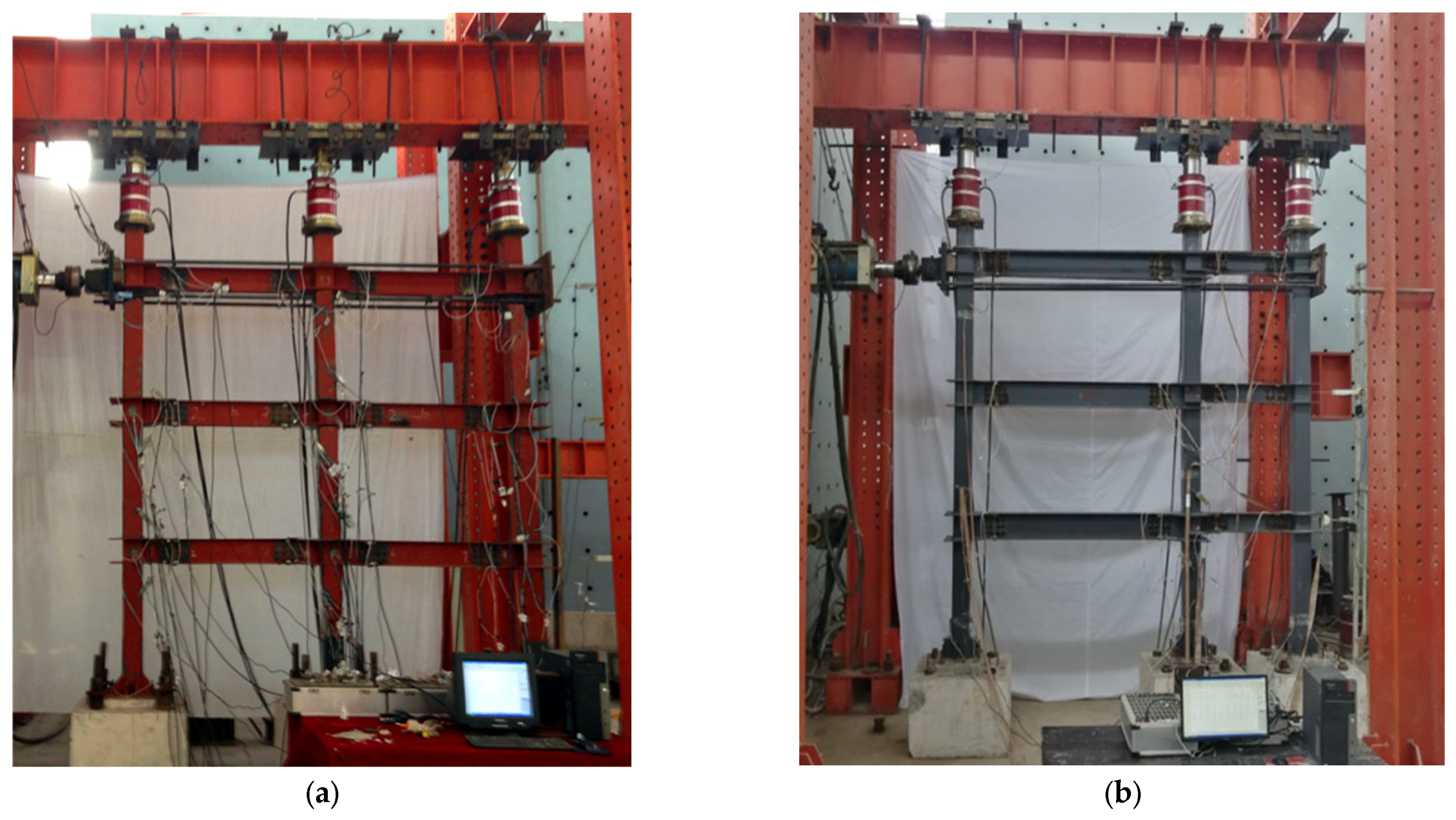
2.2. Experimental Verification and Modeling Method

The experiment results of the two 2-bay and 3-story test CFST frames tested by our group can be found in [16]. The floor height was 1 m, and the total height reached 3.3 m. The equal-span frame with a span of 1.5 m was denoted as KJE1, while the unequal-span frame with a left span of 2 m and a right span of 1 m was denoted as KJE2. The CFST column showed a cross-section size of 150 mm × 150 mm with a tube wall thickness of 6 mm. The cross-section of the steel beam of KJE1 was H180 × 90 × 6.5 × 10.7, while the cross-sections of the steel beams of KJE2 were H200 × 100 × 4.5 × 7 and H150 × 100 × 6 × 9, respectively. The concrete strength of the CFST columns was C40. The on-site photographs are shown in Figure 3, and hysteretic behavior, failure modes, and other details can be found, if interested, in [16].

OpenSees was used for modeling to simulate the hysteresis behavior of the test frames. The CFST column was simulated using the nonlinear beam–column element, since the cross-sections of the column were kept the same. The beam with hinges element offered in OpenSees could be utilized for simulating frame beams, in which different cross-sections and the existence of bolted connections could be taken into account at the beam ends [17], and the plastic hinge length was determined according to the position of the friction-type bolt at the beam end. The steel was simulated by the Steel02 model. This model, which was implemented by Menegotto and Pinto, was adopted for many types of structural steels in the simulation [18]. Considering the confinement of concrete from the tube, the Concrete02 model was used for the concrete core in the column [17]. The stress–strain relationships of concrete and steel in OpenSees are shown in Figure 4 and Figure 5, respectively.

The following assumptions were made: (1) a plane section remains planar under loading for beams and columns, (2) bond slip between the steel tube and the concrete is not taken into account, (3) the bending failure occurs before shear failure for members, and (4) no joint failure occurs during the test.

As shown in Figure 6, the shape of the simulated hysteretic curve was similar to that of the test curve. The shapes of the hysteresis curves obtained by numerical simulation were in good agreement with the experimental results, which showed that the adopted modeling method could provide a foundation for further research [19].

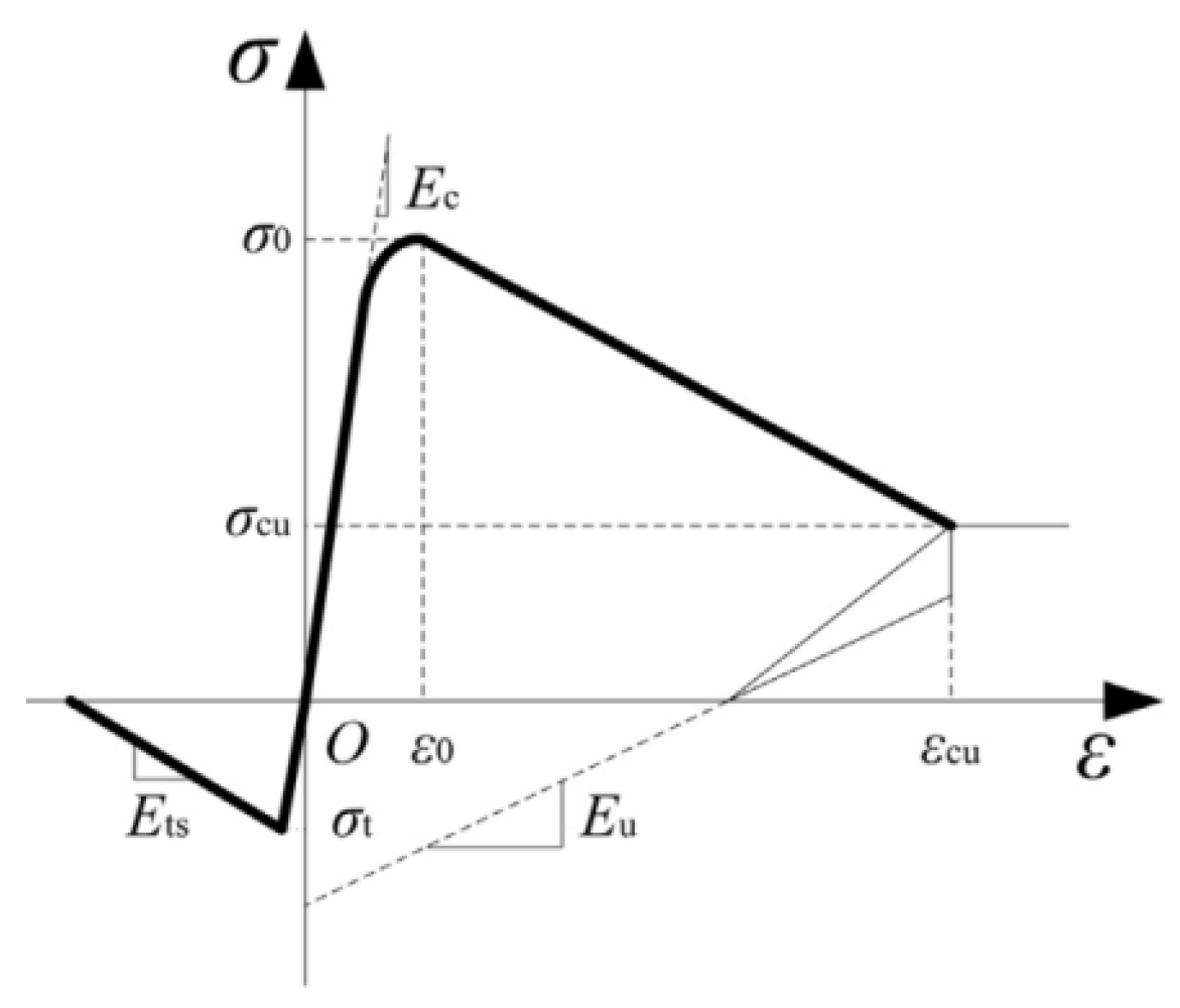
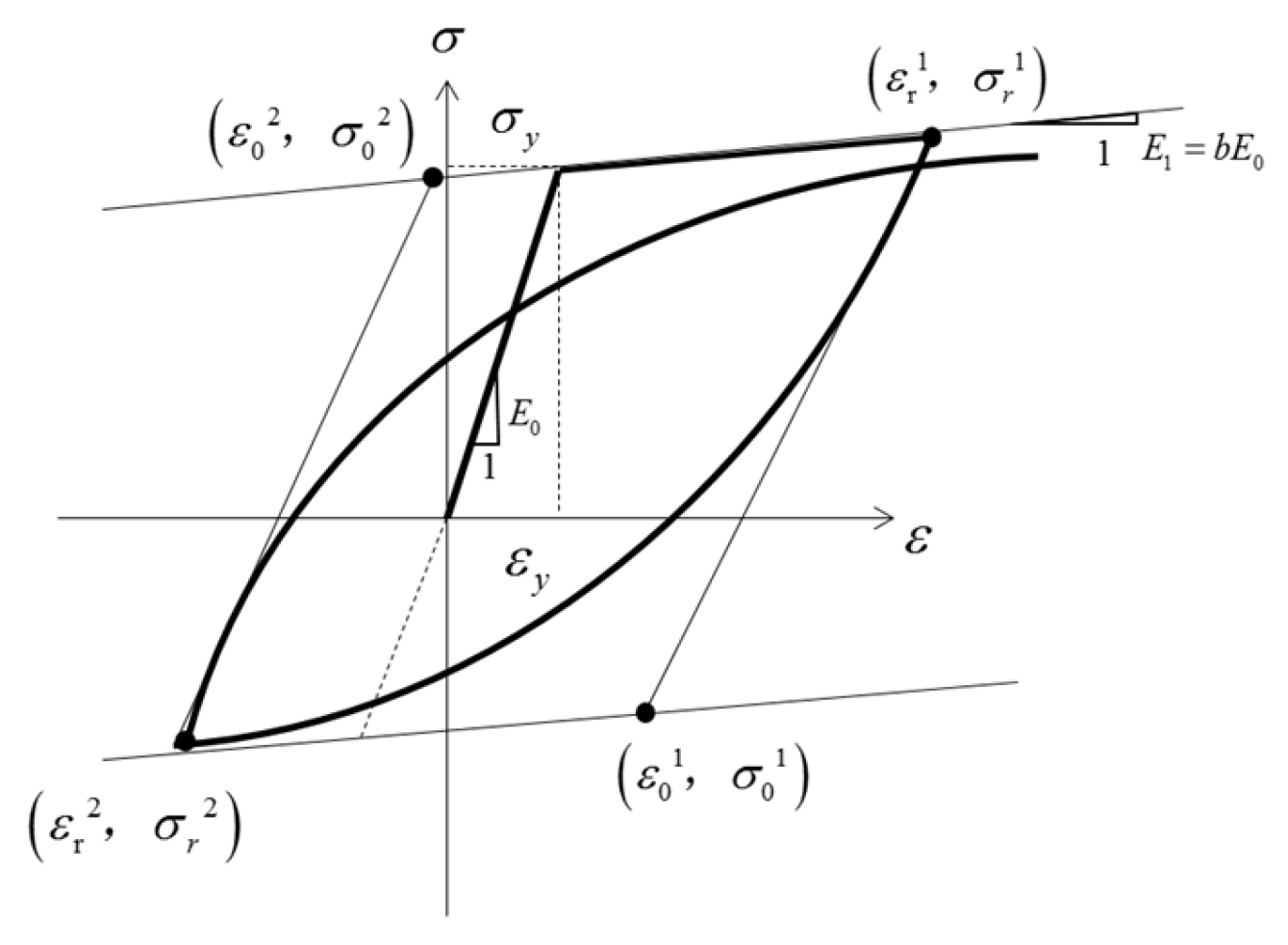
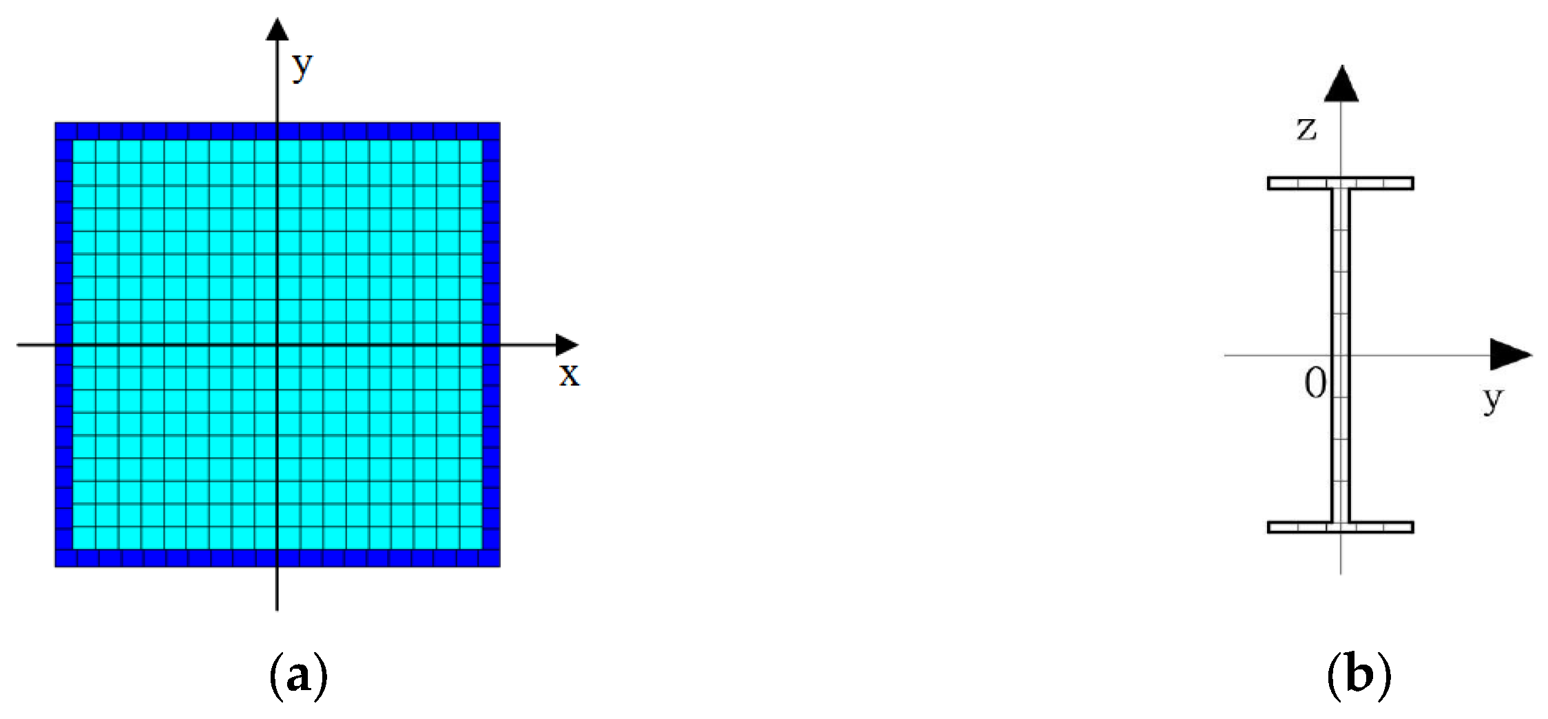
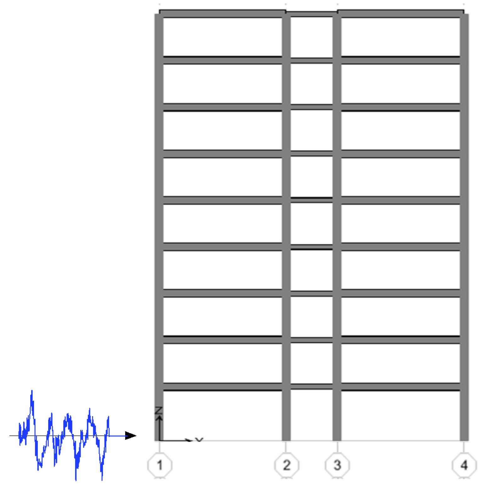
2.3. Model Establishment

A CFST plane frame model and a CFST spatial frame model were established by OpenSees according to the structural design in Section 2.1, based on the accurate simulation of the hysteresis performance of test CFST frames in Section 2.2, as shown in Figure 7. The steel was simulated by the Steel02 model, and the concrete core in the column adopted the Concrete02 model. Section division of the fiber element of the beam and column is shown in Figure 8. The CFST column was simulated using the nonlinear beam–column element, and the steel beam adopted the beam with hinges element. The modeling method and cross-section properties of each component refer to Section 2.2.

3. Incremental Dynamic Analysis

Incremental dynamic analysis is considered to be an advantageous technique, which can capture the seismic response of the designed frame archetype and evaluate the behavior of structures under different loads of seismicity. Firstly, the amplitude of ground motion is proportionally modulated to different earthquake intensities, and then the corresponding seismic response is recorded by dynamic time history analysis. Finally, the relationship line between IM of ground motions and DM of a structure is the IDA curve.

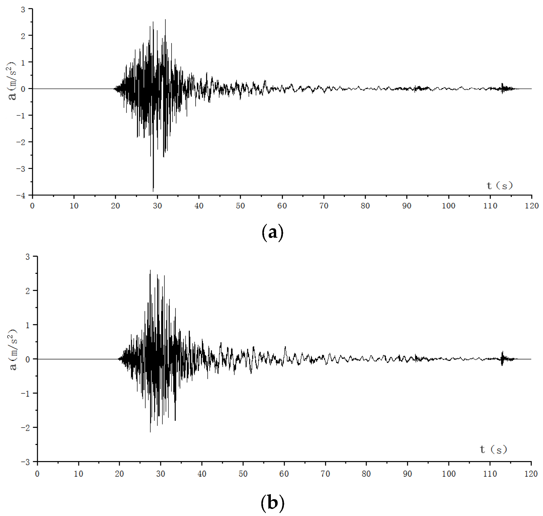
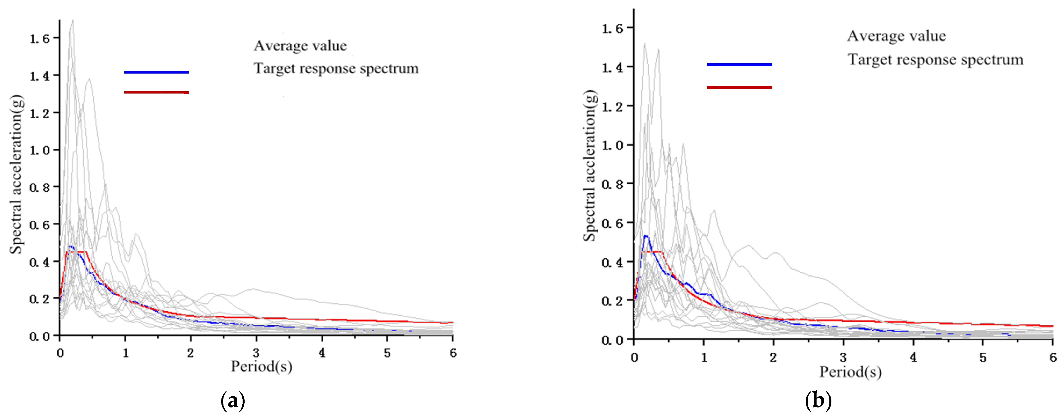
3.1. Ground Motion Selection

The authors of [4,20] indicated that IDA-based seismic fragility analysis of a mid–high-frame structure can be achieved using 10 to 20 ground motion records. Based on the site conditions (category II) and seismic fortification intensity (8°), 25 ground motion records were selected from the Pacific Earthquake Engineering Center (PEER) according to the response spectrum of GB50011-2010 “Code for Seismic Design of Buildings” [21], and the magnitude of the selected records was greater than 5.6 M. The information of ground motion is shown in

Table 2. Selected ground motions.

Record	Earthquake Name	Year	Platform	MW	Ground Motion Horizontal Component, N/E
1	“Hollister-01”	1961	Hollister City Hall	5.6	RSN26_HOLLISTR_B-HCH181/271
2	“San Fernando”	1971	Santa Felita Dam (Outlet)	6.61	RSN88_SFERN_FSD172/262
3	“Imperial Valley-06”	1979	“Cerro Prieto”	6.53	RSN164_IMPVALL.H_H-CPE147/237
4	“Irpinia_ Italy-01”	1980	“Bisaccia”	6.9	RSN286_ITALY_A-BIS000/270
5	“Chalfant Valley-02”	1986	“Long Valley Dam (Downst)”	6.19	RSN553_CHALFANT.A_A-LVD000/090
6	“Chalfant Valley-02”	1986	“Long Valley Dam (L Abut)”	6.19	RSN554_CHALFANT.A_A-LVL000/090
7	“Loma Prieta”	1989	Coyote Lake Dam—Southwest Abutment	6.93	RSN755_LOMAP_CYC195/285
8	“Manjil_ Iran”	1990	Abbar	7.37	RSN1633_MANJIL_ABBAR--L/T
9	“Cape Mendocino”	1992	Fortuna—Fortuna Blvd	7.01	RSN827_CAPEMEND_FOR000/090
10	“Cape Mendocino”	1992	Loleta Fire Station	7.01	RSN3750_CAPEMEND_LFS270/360
11	“Landers”	1992	North Palm Springs Fire Sta #36	7.28	RSN3757_LANDERS_NPF090/180
12	“Chi-Chi_ Taiwan”	1999	“TCU075”	7.62	RSN3471_CHICHI.06_TCU075 E/N
13	“Duzce_ Turkey”	1999	“Lamont 1061”	7.14	RSN1614_DUZCE_1061-N/E
14	“Chi-Chi_ Taiwan-06”	1999	“TCU075”	6.3	RSN3471_CHICHI.06_TCU075N/E
15	“San Simeon_ CA”	2003	San Antonio Dam—Toe	6.52	RSN4013_SANSIMEO_36258021/111
16	“Chuetsu-oki_ Japan”	2007	“Kawaguchi”	6.8	RSN4869_CHUETSU_65042NS/EW
17	“Chuetsu-oki_ Japan”	2007	“Ojiya City”	6.8	RSN4882_CHUETSU_65321NS/EW
18	“Chuetsu-oki_ Japan”	2007	“NIG024”	6.8	RSN5270_CHUETSU_NIG024NS/EW
19	“Chuetsu-oki_ Japan”	2007	Matsushiro Tokamachi	6.8	RSN4843_CHUETSU_65006NS/EW
20	“Chuetsu-oki_ Japan”	2007	Joetsu Ogataku	6.8	RSN4848_CHUETSU_65011NS/EW
21	“Chuetsu-oki_ Japan”	2007	Sawa Mizuguti Tokamachi	6.8	RSN4872_CHUETSU_65053NS/EW
22	“Iwate_ Japan”	2008	“Yuzawa Town”	6.9	RSN5806_IWATE_55461NS/EW
23	“Iwate_ Japan”	2008	“Kami_ Miyagi Miyazaki City”	6.9	RSN5776_IWATE_54010NS/EW
24	“Darfield_ New Zealand”	2010	“SPFS”	7	RSN6971_DARFIELD_SPFSN17E/73W
25	“Christchurch_ New Zealand”	2011	“MQZ”	6.2	RSN8110_CCHURCH_MQZE/ZN

: each ground motion record contains 2 horizontal components, and the 25 selected ground motions contain 25 motions in the X direction and 25 motions in the Y direction, named 25N and 25E, respectively.

The target response spectrum for selected ground motions with a damping ratio of 4% is shown in Figure 9, where the similar acceleration response spectrum and average value of ground motions demonstrates the accuracy of the operation.

3.2. Selection of IM and DM

The peak ground acceleration (PGA), the peak ground velocity (PGV), and the spectral acceleration value (Sa) are often used as the intensity measures (IM) of ground motions. The authors of [22] suggested that PGA is relatively superior, which is consistent with the current seismic code in China. The peak inter-story drift ratio limit (θ_max) has the advantages of simple calculation and convenient application, which is directly related to the deformation capacity of buildings, and θ_max was selected as the quantitative limit of the structure under different performance levels in domestic and foreign specifications. In this paper, PGA was chosen as the IM and θ_max was chosen as the demand measure (DM), and the PGA of the selected ground motions scaled from 0.1 g to 2.0 g, with an interval of 0.2 g.

According to ATC-40 and GB/T 24335-2009, θ_max was selected as the damage state to classified the performance level, where slight damage, moderate damage, and extensive damage correspond to characteristic points of the pseudo-static frame test, and the characteristic points include the yield point, maximum load point, and ultimate load point [16,23]. When θ_max is greater than 0.1, the structure is considered as collapsed or complete damage [24]. The θ_max values of the damage state were obtained based on the statistical data and relevant specifications, as shown in

Table 3. Inter-story drift ratio limits of damage state for the CFST frame structure.

Damage State	Slight Damage (LS1)	Moderate Damage (LS2)	Extensive Damage (LS3)	Complete Damage (LS4)
θmax	1/150	1/50	1/30	1/10

.

3.3. Analysis and Discussion of IDA Results

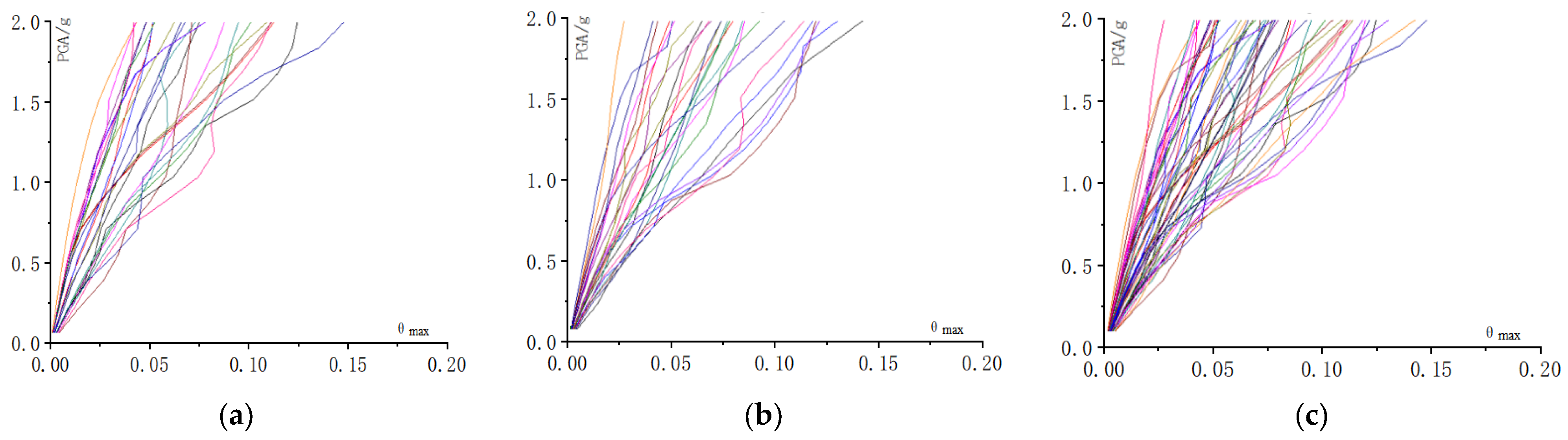
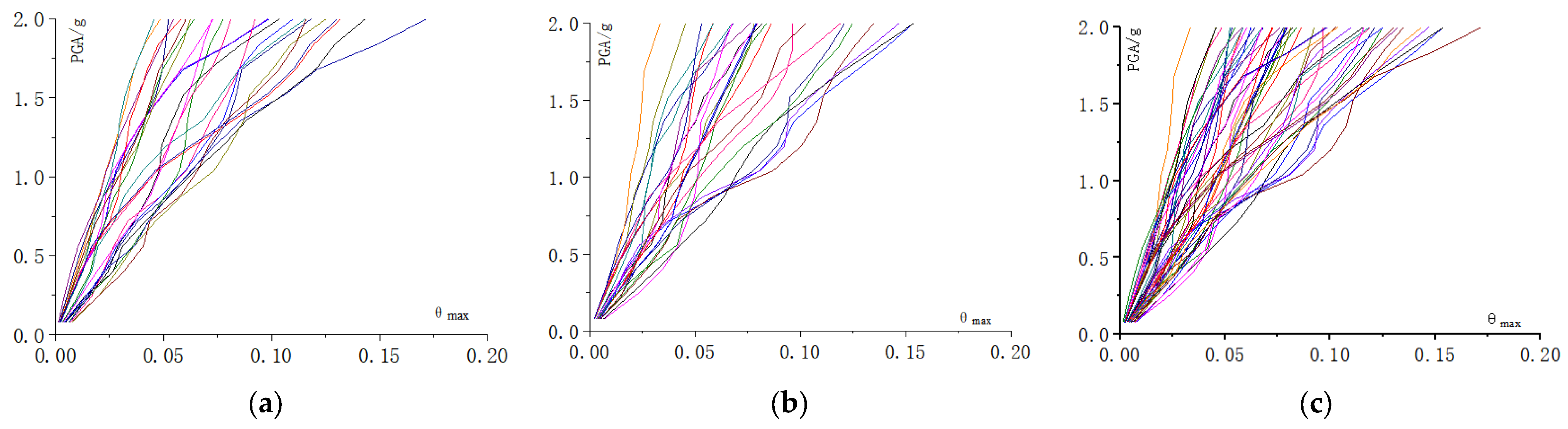
3.3.1. IDA Curve Clusters of In-Plane Frame

Figure 10 shows the plane frame subjected to 1D ground motions. It was calculated that the θ_max of the plane frame models obtained from OpenSees was on the third floor or the fourth floor. IDA curve clusters of the plane frame subjected to 1D ground motions are shown in Figure 11a,b. Figure 11c shows IDA curve clusters of the in-plane frame subjected to 50 1D ground motions. With the increase in PGA, the slope of each curve decreased gradually, but the monotone increasing phenomenon did not always occur, and part of the IDA curves had states including “softening” and “zigzagging”.

3.3.2. IDA Curve Clusters of Spatial Frame Subjected to 1D Ground Motions

Figure 12 shows the spatial frame subjected to 1D ground motions, and the weak axis direction (Y direction) of the spatial frame was taken as the main horizontal direction. IDA curve clusters of the spatial frame subjected to 1D ground motions are shown in Figure 13a–c. The comparison between Figure 11 and Figure 13 showed that the difference between IDA curves of the spatial frame and plane frame for the same structural model subjected to 1D ground motions was significant. The average θ_max of the spatial frame subjected to 1D ground motions was 10–20% larger than that of the plane frame. That is to say, the seismic response results of the plane frame were not enough to evaluate the seismic performance of the structure.

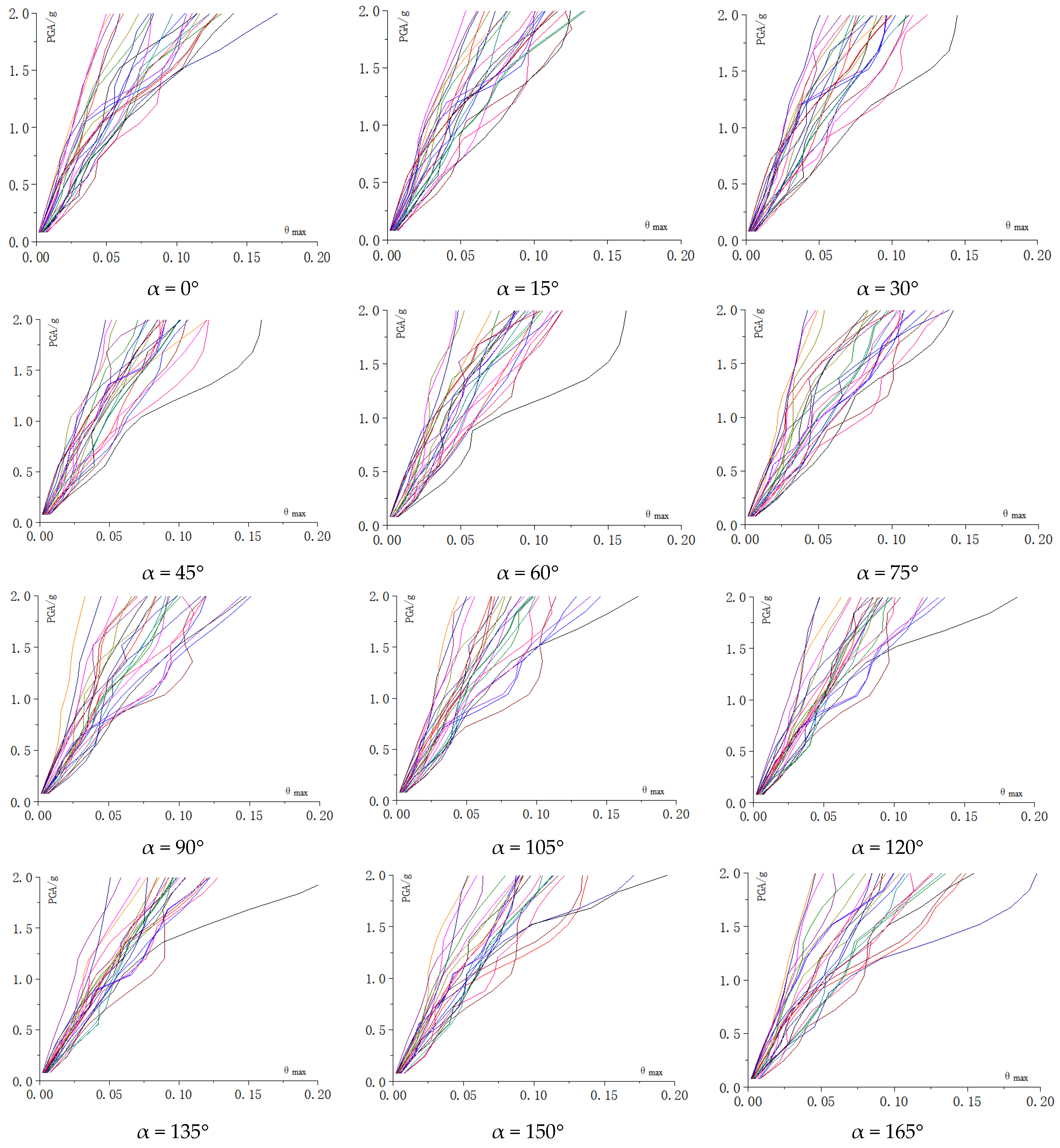
3.3.3. IDA Curve Clusters of Spatial Frame Subjected to 2D Ground Motions Considering Attacking Angle

Figure 14 shows the spatial frame subjected to 2D ground motions considering 13 attacking angles, where the angle α is 0 to 180 degrees with the spacing of 15 degrees, while 0° represents the attacking angle of original ground motion. As shown in Figure 14, the black arrow line represents the attacking direction of the original ground motion, and the green arrow line represents the attacking direction of the ground motion at the angles of α.

The inter-story drift ratios of each joint of the frame along the X and Y directions should be recorded, respectively, and then the θ_max should be found by calculating according to the following formula:

$$\theta =\sqrt{{\theta }_x^2+{\theta }_y^2}$$

(1)

where, θ_x and θ_y are inter-story drift ratios of any joint along the X and Y directions, respectively.

The magnitude of peak acceleration will not completely determine the seismic response of the spatial frame, while the structural properties of the weak axis direction and the strong axis direction, the discount coefficient of the second horizontal component of ground motion, and the coupling effects in the two axis directions all affect the calculation results. By transforming the attacking angle of the ground motions, the sample of ground motion was greatly increased. IDA clusters of the spatial frame subjected to 2D ground motions under the different attacking angles are listed in Figure 15.

In order to understand the influence of the attacking angle of ground motion on the θ_max of the frame, the average value of θ_max corresponding to each group of different attacking angles was used to compare the baseline of $\overline{\theta }$_max,α=0° in Figure 16. A certain trend can be found: When the attacking angle was 15°–45°, there was little difference between $\overline{\theta }$_max and θ_max,α=0°. When the attacking angle was 60°–120°, PGA < 1.5 g, the value of $\overline{\theta }$_max was greater than that of θ_max,α=0°. When PGA > 1.5 g, $\overline{\theta }$_max was less than $\overline{\theta }$_max,α=0°. At the attacking angles of 135°, 150°, and 165°, all the values of $\overline{\theta }$_max were greater than that of $\overline{\mathrm{\theta }}$_max,α=0°. When PGA = 0.75 g, the difference between $\overline{\theta }$_max and $\overline{\theta }$_max,α=0° was the largest. The value of θ_max,α=180° coincided almost exactly with that of $\overline{\theta }$_max,α=0°. In general, the seismic response was found to be sensitive to the attacking angle of ground motion.

4. Seismic Fragility Analysis

4.1. Probabilistic Seismic Demand Model (PSDM)

IDA curves in Section 3 were used to establish the probabilistic seismic demand model between DM and IM. The regression formulas between PGA and θ_max can be expressed as follows:

ln(θ_max) = aln(PGA) + b

(2)

where a and b are regression parameters.

According to the linear regression formula above, the regressions of the PSDM of CFST frames are listed in

Table 4. The fitting formula between θ_max and PGA.

Structure	Ground Motions	Attacking Angle	The Linear Regression Formula
Plane frame subjected to 1D ground motions	25(N)	0°	ln(EDP) = 1.133238ln(IM) − 3.69704
	25(E)	0°	ln(EDP) = 1.093857ln(IM) − 3.599816
	50(25N + 25E)	0°	ln(EDP) = 1.113548ln(IM) − 3.648429
Spatial frame subjected to 1D ground motions	25(N)	0°	ln(EDP) = 1.015568ln(IM) − 3.445141
	25(E)	0°	ln(EDP) = 0.9599472ln(IM) − 3.364997
	50(25N + 25E)	0°	ln(EDP) = 0.9875820ln(IM) − 3.405069
Spatial frame subjected to 2D ground motions	25N + 25E	0°	ln(EDP) = 1.011276ln(IM) − 3.343988
	25N + 25E	15°	ln(EDP) = 1.006654ln(IM) − 3.356569
	25N + 25E	30°	ln(EDP) = 0.986977ln(IM) − 3.37602
	25N + 25E	45°	ln(EDP) = 0.975368ln(IM) − 3.354419
	25N + 25E	60°	ln(EDP) = 0.958666ln(IM) − 3.321175
	25N + 25E	75°	ln(EDP) = 0.952800ln(IM) − 3.293288
	25N + 25E	90°	ln(EDP) = 0.946490ln(IM) − 3.317331
	25N + 25E	105°	ln(EDP) = 0.958472ln(IM) − 3.328774
	25N + 25E	120°	ln(EDP) = 0.973446ln(IM) − 3.310517
	25N + 25E	135°	ln(EDP) = 0.995960ln(IM) − 3.275722
	25N + 25E	150°	ln(EDP) = 0.995817ln(IM) − 3.273766
	25N + 25E	165°	ln(EDP) = 1.001221ln(IM) − 3.295428
	25N + 25E	180°	ln(EDP) = 1.012651ln(IM) − 3.342390
	(25N + 25E) × 13	All	ln(EDP) = 0.981602ln(IM) − 3.32366

. The PSDMs of the plane frame, spatial frame subjected to 1D ground motions, and spatial frame subjected to 2D ground motions were quite different, and the PSDM of spatial frame was also different under different attacking angles.

4.2. Seismic Fragility Curves

Seismic fragility analysis is the probability that the seismic response of a building will reach or exceed a certain performance level limit under different seismic effects. When IM = a, the exceeding probability exceeding the limit state value, C, is expressed as follows:

$$F(a)=P(\mathrm{DM}>=C/IM=a)$$

(3)

Therefore, F(a) can be then calculated according to Equation (3), according to the relationship between IM and DM:

$$F(a)=P(\mathrm{DM}>C/IM=a)=\Phi \left[{\displaystyle \frac{\ln (\overline{\mathrm{DM}}/C)}{\sqrt{{\beta }_{EDP}^2+{\beta }_c^2}}}\right]$$

(4)

where, ${\beta }_{DM}$ and ${\beta }_C$ are the logarithmic standard deviation of the structural seismic response and critical value of failure state, respectively. The value of $\sqrt{{\beta }_{\mathrm{DM}}^2+{\beta }_c^2}$ is related to the seismic intensity index, the spectral acceleration was 0.4, and the peak acceleration was 0.5 [22]. The exceeding probability curve can be further obtained from the equation, which is the fragility curve, and the curve transitions from steep to gradual as the damage progresses from slight damage to near collapse.

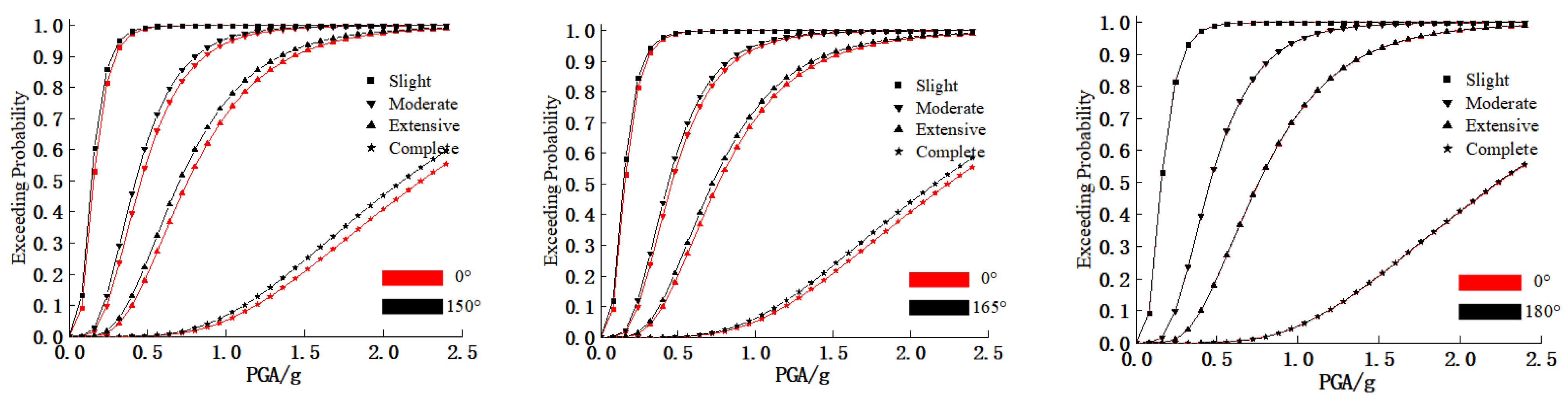
4.3. Effect of the Attacking Angle on Seismic Fragility

Figure 17 presents the comparison of seismic fragility curves between different attacking angles and 0° (original attacking angle).

When the attacking angle was 15–45°, the exceeding probability of fragility curves at the three performance levels (LS1–LS3) was close to that of the 0° fragility curves, and the exceeding probability of the 0° fragility curves in LS4 was larger than that of the others. When the attacking angle was 60–90°, the exceeding probability of fragility curves at the three performance levels (LS1–LS3) was larger than that of the 0° fragility curves, while the exceeding probability was close to that of the 0° fragility curves in LS4. The exceeding probability of the 135°, 150°, and 165° fragility curves was larger than that of the 0° fragility curves at each performance level. The 180° fragility curve coincided perfectly with the 0° fragility curves. In general, the exceeding probability was found to be sensitive to the attacking angle of ground motion, and the seismic fragility analysis did not only focus on the original attacking angle, but also considered the adverse effects of different attacking angles.

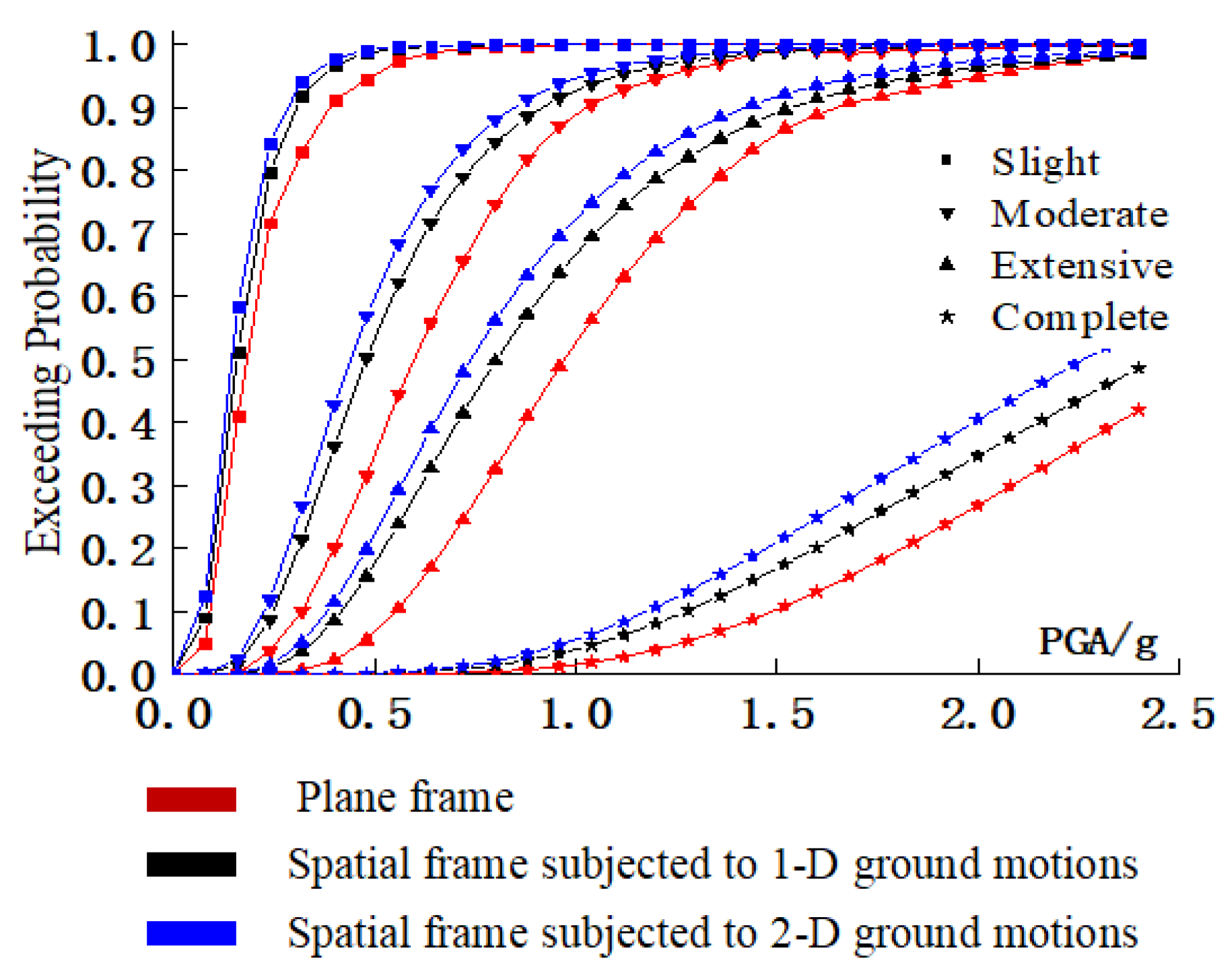
4.4. The Comparison of Fragility Analysis Curves of CFST Plane Frame and Spatial Frame

The comparison of fragility analysis curves is shown in Figure 18. The red line represents the seismic fragility analysis results of the in-plane frame subjected to 1D ground motions (25N + 25E) at 10 intensities, so that, in total, 500 (=50 × 10) nonlinear dynamic analyses were performed. The black line represents the seismic fragility analysis results of the spatial frame subjected to 1D ground motions (25N + 25E) at 10 intensities, in a total of 500 (=50 × 10) analyzed cases. The blue line represents the seismic fragility analysis results of the spatial frame subjected to 2D ground motions (25N + 25E) at 10 intensities considering 13 attacking angles, in a total of 3250 (=25 × 10 × 13) analyzed cases.

At the LS1 level, the fragility curves of the spatial frame subjected 2D ground motions and 1D ground motions almost coincided, and the exceeding probability of the spatial frame was larger than that of the plane frame. At the level of damage state from LS1 to near collapse, the fragility curves showed obvious characteristics. The exceeding probability of the spatial frame subjected to 2D ground motions at each performance level was successively greater than that of the 1D ground motion, and greater than that of the plane frame. This shows that for 2D earthquakes, it is easier to motivate the frame structure to exceed a certain damage state. As shown in

Table 5. The exceeding probabilities of the CFST frame under PGA of 0.2 g.

	Damage State
	LS1	LS2	LS3	LS4
Plane frame	0.586	0.019	0.002	0
Spatial frame subjected to 1D ground motions	0.667	0.051	0.005	0
Spatial frame subjected to 2D ground motions	0.735	0.072	0.008	0

and

Table 6. The exceeding probabilities of the CFST frame under PGA of 0.3 g.

	Damage State
	LS1	LS2	LS3	LS4
Plane frame	0.806	0.083	0.004	0
Spatial frame subjected to 1D ground motions	0.890	0.182	0.0285	0
Spatial frame subjected to 2D ground motions	0.919	0.228	0.0416	0

, when the structure was under the intensity level of frequent earthquakes (PGA = 0.2 g), the exceeding probability of the spatial frame subjected to 2D ground motions was close to 73% in the slight damage state, while the exceeding probability of the plane frame was close to 59%. In the moderate damage state, the exceeding probability of spatial frame subjected to 2D ground motions was 50% higher than that of the plane frame. When PGA = 0.3 g, the exceeding probability of spatial frame was 10% higher than that of plane frame. In addition, from LS2 to near LS4, the difference in seismic fragility curves was gradually enlarged. This shows that the spatial frame subjected to 2D ground motions is more likely to cause more severe damage to the structure under a large earthquake intensity. Therefore, when the IDA-based seismic fragility method is employed to evaluate the seismic performance of the CFST frame structure, it is necessary to adopt the spatial frame and consider bidirectional inputs of ground motions.

5. Conclusions

In this paper, we conducted seismic fragility analysis of a nine-story CFST plane frame and spatial frame employing the IDA method. Based on the analysis results, the following conclusions can be summarized:

(1)

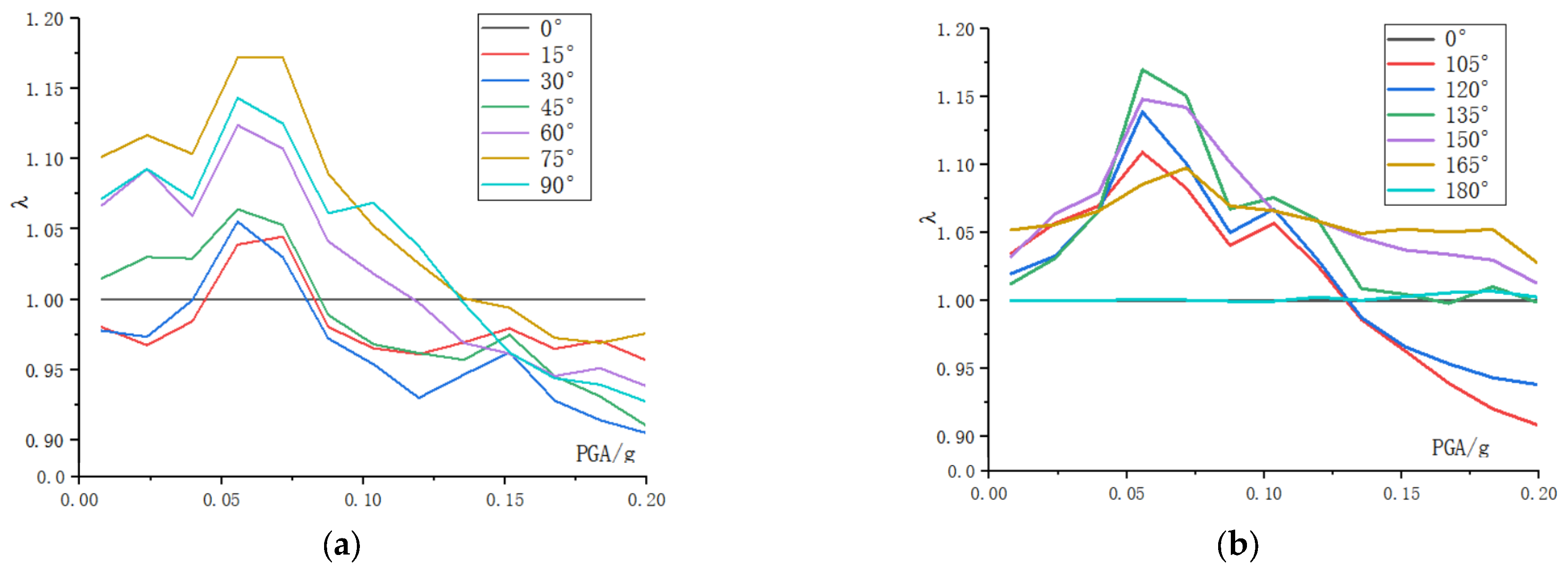
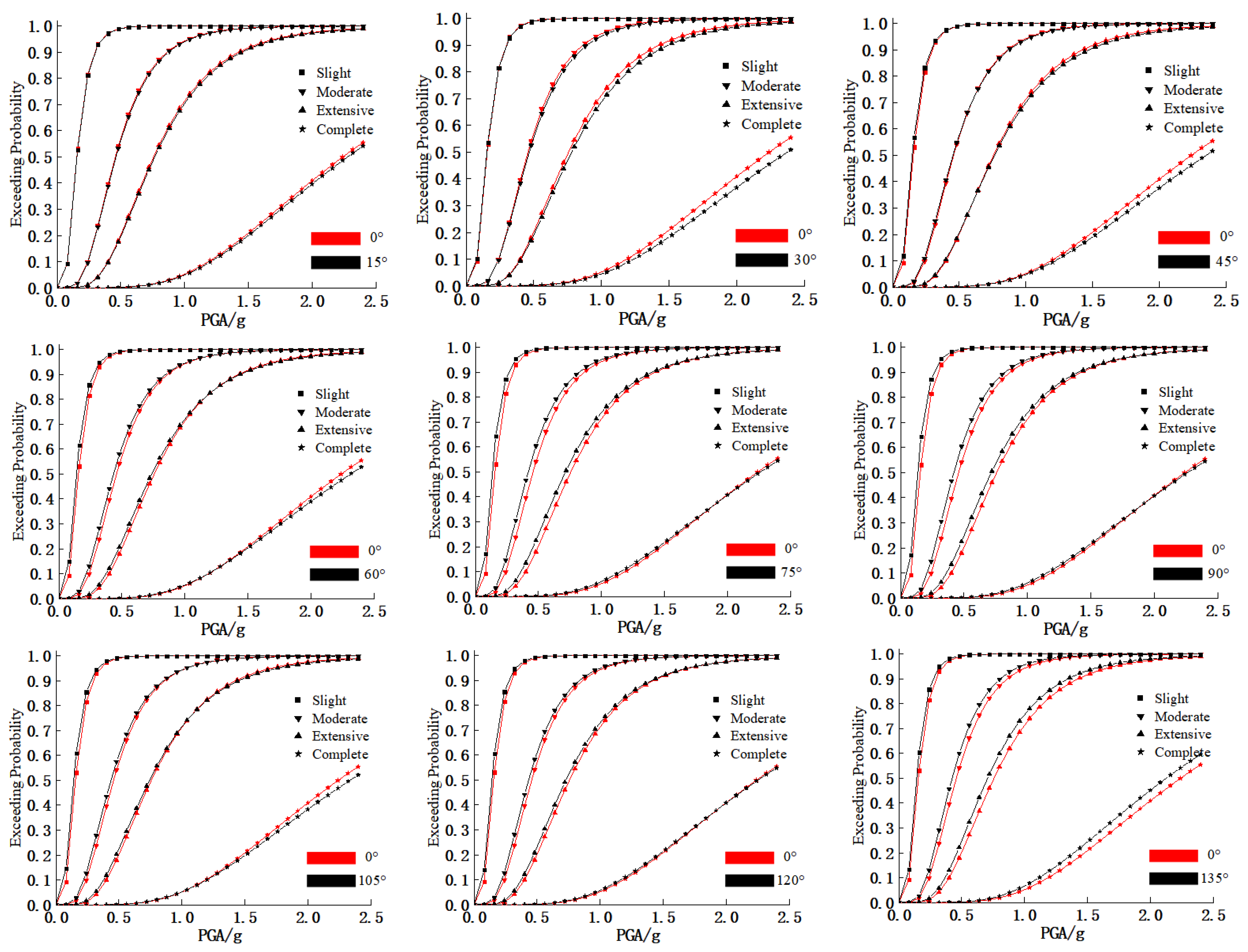
For the CFST spatial frame under 2D ground motions, the seismic fragility analysis result was found to be sensitive to the attacking angle of ground motion, where the exceeding probability of the 15°, 30°, and 45° fragility curves at the levels LS1–LS3 was close to that of the 0° fragility curves, the exceeding probability of the 60°–90° fragility curves at the levels LS1–LS3 was larger than that of the 0° fragility curves, and the exceeding probability of the 135°, 150°, and 165° fragility curves was larger than that of the 0° fragility curves at each performance level.

(2)

The results of the seismic fragility analysis of the spatial frame were obviously different from those of the plane frame. The analytical results showed that the exceeding probability of the spatial frame under 2D ground motions was successively greater than that under 1D ground motions, and greater than the plane frame, and the maximum difference at each performance level was up to 6% and 16%, respectively.

(3)

IDA-based seismic fragility analysis of CFST frames should adopt the spatial frame model and consider the effect of the attacking angle of 2D ground motions, rather than the plane frame model.

References

1. Cheng, Y.; Dong, Y.-R.; Bai, G.-L.; Wang, Y.-Y. IDA-based seismic fragility of high-rise frame-core tube structure subjected to multi-dimensional long-period ground motions. J. Build. Eng. 2021, 43, 102917. [Google Scholar] [CrossRef]
2. Rajkumari, S.; Thakkar, K.; Goyal, H. Fragility analysis of structures subjected to seismic excitation: A state-of-the-art review. Structures 2022, 40, 303–316. [Google Scholar] [CrossRef]
3. Wang, J.; Sun, Y. Seismic fragility and post-earthquake reparability of concrete frame with low-bond high-strength reinforced concrete column. Structures 2022, 37, 185–202. [Google Scholar] [CrossRef]
4. Rezaei, H.; Zarfam, P.; Golafshani, E.M.; Amiri, G.G. Seismic fragility analysis of RC box-girder bridges based on symbolic regression method. Structures 2022, 38, 306–322. [Google Scholar] [CrossRef]
5. Jia, D.-W.; Wu, Z.-Y. Seismic fragility analysis of RC frame-shear wall structure under multidimensional performance limit state based on ensemble neural network. Eng. Struct. 2021, 246, 112975. [Google Scholar] [CrossRef]
6. Bao, C.; Ma, X.; Lim, K.S.; Chen, G.; Xu, F.; Tan, F.; Hamid, N.H.A. Seismic fragility analysis of steel moment-resisting frame structure with differential settlement. Soil Dyn. Earthq. Eng. 2021, 141, 106526. [Google Scholar] [CrossRef]
7. Xu, C.; Guo, C.; Xu, Q.; Yang, Z. The global collapse resistance capacity of a seismic-damaged SRC frame strengthened with an enveloped steel jacket. Structures 2021, 33, 3433–3442. [Google Scholar] [CrossRef]
8. Vasileiadis, V.; Kostinakis, K.; Athanatopoulou, A. Story-wise assessment of seismic behavior and fragility analysis of R/C frames considering the effect of masonry infills. Soil Dyn. Earthq. Eng. 2023, 165, 107714. [Google Scholar] [CrossRef]
9. Mansouri, I.; Hu, J.W.; Shakeri, K.; Shahbazi, S.; Nouri, B. Assessment of seismic vulnerability of steel and RC moment buildings using HAZUS and statistical methodologies. Discret. Dyn. Nat. Soc. 2017, 2017, 2698932. [Google Scholar] [CrossRef]
10. Qu, Z.; Ye, L.; Pan, P. Comparative study on methods of selecting earthquake ground motions for nonlinear time history analyses of building structures. China Civ. Eng. J. 2011, 44, 10–21. [Google Scholar]
11. Yang, F.; Gao, X.; Zhang, W. Rasponse of tall-building steel structure to muti-dimensional seismic action. J. Build. Struct. 2003, 24, 33–43. [Google Scholar]
12. Kostinakis, K.; Morfidis, K.; Xenidis, H. Damage response of multistorey r/c buildings with different structural systems subjected to seismic motion of arbitrary orientation. Earthq. Eng. Struct. Dyn. 2015, 44, 1919–1937. [Google Scholar] [CrossRef]
13. Lagaros, N.D. Multicomponent incremental dynamic analysis considering variable incident angle. Struct. Infrastruct. Eng. 2010, 6, 77–94. [Google Scholar] [CrossRef]
14. GB50936-2014; Technical Code for Concrete Filled Steel Tubular Structures. Ministry of Housing and Urban-Rural Development of the People’s Republic of China: Beijing, China, 2014.
15. JGJ138-2016; Code for the Design of Composite Structures. Ministry of Housing and Urban-Rural Development of the People’s Republic of China: Beijing, China, 2016.
16. Liu, X.; Xu, C.; Peng, S.; Zhou, B. Influence of staggered floor and unequal height of left and right beam on seismic behavior of CFSST column-to-HSS beam composite frames. J. Build. Eng. 2023, 66, 105878. [Google Scholar] [CrossRef]
17. Wang, K.; Lu, X.-F.; Yuan, S.-F.; Cao, D.-F.; Chen, Z.-X. Analysis on hysteretic behavior of composite frames with concrete-encased CFST columns. J. Constr. Steel Res. 2017, 135, 176–186. [Google Scholar] [CrossRef]
18. Zhang, Z.; Wang, J.; Li, B.; Zhao, C. Seismic tests and numerical investigation of blind-bolted moment CFST frames infilled with thin-walled SPSWs. Thin Walled Struct. 2019, 134, 347–362. [Google Scholar] [CrossRef]
19. Chen, J.; Bian, Y.; Su, L. Application of OpenSees on calculating lateral force-displacement hysteretic curves of concrete-filled steel tubular frame with unequal spans. World Earthq. Eng. 2021, 37, 111–118. [Google Scholar]
20. Xu, C.; Deng, J.; Peng, S.; Li, C. Seismic fragility analysis of steel reinforced concrete frame structures based on different engineering demand parameters. J. Build. Eng. 2018, 20, 736–749. [Google Scholar] [CrossRef]
21. GB/T50011-2010; Code for Seismic Design of Buildings. Ministry of Housing and Urban-Rural Development of the People’s Republic of China: Beijing, China, 2024.
22. Karafagka, S.; Fotopoulou, S.; Pitilakis, D. Fragility assessment of non-ductile RC frame buildings exposed to combined ground shaking and soil liquefaction considering SSI. Eng. Struct. 2021, 229, 111629. [Google Scholar] [CrossRef]
23. Research on Seismic Behavior and Design Method of Composite Frame with Reinforced Concrete Columns and Steel Beams; Xi’an University of Architecture and Technology: Xi’an, China, 2014.
24. Jalali, S.A.; Amini, A.; Mansouri, I.; Hu, J.W. Seismic collapse assessment of steel plate shear walls considering the mainshock–aftershock effects. J. Constr. Steel Res. 2021, 182, 106688. [Google Scholar] [CrossRef]
Figure 1. Acceleration time histories of “RSN3471_CHICHI.06_TCU075”. (a) Horizontal component E. (b) Horizontal component N.
Buildings 14 02686 g001
Figure 2. Structure plan view (unit: mm).
Buildings 14 02686 g002
Figure 3. On-site photographs. (a) KJE1 and (b) KJE2.
Buildings 14 02686 g003
Figure 4. Concrete02 stress–strain curve.
Buildings 14 02686 g004
Figure 5. Steel02 stress–strain curve.
Buildings 14 02686 g005
Figure 6. Comparison of hysteresis curves. (a) KJE1 and (b) KJE2.
Buildings 14 02686 g006
Figure 7. Frame models. (a) Plane frame model and (b) spatial frame model.
Buildings 14 02686 g007
Figure 8. Component cross-section. (a) Column and (b) beam.
Buildings 14 02686 g008
Figure 9. Response spectra of the selected ground motion records. (a) Horizontal component, N, and (b) horizontal component, E.
Buildings 14 02686 g009
Figure 10. Plane frame subjected to 1D ground motions.
Buildings 14 02686 g010
Figure 11. IDA curve clusters of the in-plane frame: (a) 25N, (b) 25E, and (c) 25N + 25E.
Buildings 14 02686 g011
Figure 12. Spatial frame subjected to 1D ground motions.
Buildings 14 02686 g012
Figure 13. IDA curve clusters of the spatial frame subjected to 1D ground motions: (a) 25N, (b) 25E, and (c) 25N + 25E.
Buildings 14 02686 g013
Figure 14. Spatial frame subjected to 2D ground motions considering the attacking angle.
Buildings 14 02686 g014
Figure 15. IDA curve clusters of the spatial frame subjected to 2D ground motions with different attacking angles.
Buildings 14 02686 g015
Figure 16. Comparison of θ ¯ max of different attacking angles: (a) 0°–90° and (b) 105°–180°.
Buildings 14 02686 g016
Figure 17. Seismic fragility curves of the spatial frame subjected 2D ground motions of different attacking angles.
Buildings 14 02686 g017aBuildings 14 02686 g017b
Figure 18. Fragility analysis curves of the CFST plane frame and spatial frame.
Buildings 14 02686 g018