Abstract
To investigate the impact of freeze–thaw damage on the mechanical properties of concrete, this study utilized Python in combination with ABAQUS 2016 to generate a two-dimensional meso-scale model of concrete. Uniaxial compression tests were conducted on the concrete after freeze–thaw cycles to study the evolution of its mechanical properties. Using “relative compressive strength” as a variable, the relationships between this variable and the parameters of the freeze–thaw damage model were determined, leading to the establishment of the freeze–thaw damage model and the simulation of compressive tests on concrete after freeze–thaw cycles. This study also explored the changes in the mechanical properties of concrete with variations in ITZ parameters and coarse aggregate content. The conclusions drawn are as follows: A comparison with experimental data showed that the model ensures that the relative error of each mechanical property parameter does not exceed 7%, verifying the model’s rationality. Increasing the ratio of ITZ parameters improved the mechanical properties of the ITZ, enhancing the overall mechanical performance, but had almost no effect on the elastic modulus. Compared to ratios of 0.7 and 0.8, concrete with a ratio of 0.9 showed slower rates of decrease in compressive strength and elastic modulus and slower rates of increase in peak compressive strain after freeze–thaw cycles. The increase in coarse aggregate content had a similar effect on the strength and freeze–thaw resistance of concrete as the ratio of ITZ parameters. Concrete with a coarse aggregate content of 60% exhibited slower rates of change in mechanical properties after freeze–thaw cycles.
1. Introduction
With the advent of industrialization and urbanization, the construction industry consumes vast amounts of natural resources and energy while generating significant amounts of waste. However, the multifunctionality and cost effectiveness of concrete make it the most commonly used material in the construction industry [1,2,3]. The issue of freeze–thaw damage is prevalent in concrete, and, therefore, through mesoscopic research on concrete, it is possible to accurately simulate the stress–strain development of the material during loading/unloading processes, thus providing a true reflection of the material’s mechanical properties [4]. From a mesoscopic perspective, when freeze–thaw-damaged concrete is subjected to external loads, cracks initiate from the ITZ, similar to undamaged concrete, and gradually propagate into the mortar, ultimately leading to the failure of the concrete [5]. Considering the mesoscopic characteristics of concrete allows for a more effective and accurate understanding of the expansion of internal cracks in concrete. Consequently, this enables a more effective and accurate analysis of the changes in mechanical properties at the macroscopic level [6].
In recent years, many scholars have conducted experiments on concrete in order to explain the mechanisms of freeze–thaw damage, yielding several conclusions. Chatterji [7] proposed the frost heave pressure hypothesis, which suggests that water first freezes on the outer surface and then spreads inward, causing the concrete to expand in volume. When the pressure generated reaches a critical value, it damages the concrete. Deng et al. [8] found that, with an increasing number of F-T cycles, the proportions of medium and large pores and cracks with radii greater than 1 μm in concrete increase, while the proportions of micropores and mesopores with radii smaller than 0.01 μm decrease. This indicates that the internal structure of the concrete becomes progressively loose, leading to declines in mechanical properties. Luo et al. [9] discovered that freeze–thaw cycles have a more significant impact on the internal micropores and microcracks of concrete. As the number of cycles increases, more pores and cracks form, accumulate, and expand within the cement paste and aggregate, ultimately causing the concrete material to fail. As research has progressed, many researchers have begun to investigate the mechanical behaviors of the interface between aggregates and cement paste (Interfacial Transition Zone). He et al. [10] argued that the ITZ is the most critical component of concrete and represents its weakest link, determining the performance degradation of concrete. Golewski [11] found that environmental exposure of concrete structures alternates between water-saturated and -unsaturated conditions, and dynamic loads can exacerbate cracks in the ITZ and the concrete itself. Maruyama et al. [12] noted the presence of numerous primary cracks and voids in the ITZ. Cracks in concrete often initiate and propagate along the ITZ, reducing the mechanical properties of the concrete. Thus, after freeze–thaw cycles, internal cracks are likely to start from the ITZ and extend until the entire structure is compromised.
With the rapid development of computer technology and the continuous improvement of numerical computation methods, mesoscopic numerical simulation research on concrete is increasingly becoming the mainstream approach. Compared to traditional experimental methods, mesoscopic numerical simulation offers advantages such as low cost, short-time consumption, and convenient data acquisition, and, thus, it has been widely promoted in concrete material research and engineering applications [13]. Jin et al. [14] established a diffusion-reaction-damage mesoscopic simulation for the sulfate ion erosion process inside concrete based on damage functions and Fick’s second law, considering the chemical reaction of sulfate ion transport. Wu et al. [15] constructed a stochastic convex polygon aggregate model to analyze and predict the deterioration of concrete under salt erosion. They proposed a finite element method to numerically analyze the erosion of concrete by sulfate ions, examining the variations of sulfate ions and expansion products at meso-scale conditions. A variable coefficient transport model for sulfate and chloride ions in concrete was developed by Dong et al. [16], integrating the principles of mass conservation, Fick’s second law, and porous media theory. This model comprehensively accounts for chloride ion adsorption and desorption during transport and sulfate ion reaction and hydration product filling processes, as well as the significant influences of porosity and tortuosity on ion transport. Gan et al. [17] proposed a novel mesoscopic numerical model for concrete by combining pore expansion theory, the damage plasticity model, and the element removal technique to investigate the compressive performance of concrete in freeze–thaw environments. Miao et al. [18] used the Abaqus thermo-mechanical-coupled meso-scale numerical analysis platform to conduct a parametric study on the damage process of concrete with porosity and aggregate grading defects under freeze–thaw cycles. To determine the depths of partial carbonation and complete carbonation of concrete under sustained loading, Shi et al. [19] proposed a numerical method. This method modifies the diffusion rate of each element based on the levels of multiaxial stress and stress damage.
Currently, the majority of research techniques used to assess the mechanical properties of concrete subjected to freeze–thaw damage involve macroscopic physical experiments. Liu et al. [20] conducted uniaxial compression tests to investigate the complete load–deformation curves, failure process, and failure modes of concrete prismatic specimens. They also analyzed the peak compressive stress, elastic modulus, peak compressive strain, and ultimate compressive strain at different strengths and replacement rates. Biaxial compression tests on concrete after freeze–thaw cycles were conducted to analyze the dependence of ultimate strength on the number of freeze–thaw cycles and the relationship between the number of freeze–thaw cycles, the stress ratio, and the strain rate based on experimental data from Wang et al. [21]. Zhang et al. [22] investigated the compressive strength of foam concrete with different densities under the influence of single factors (such as water immersion, constant compression load, and freeze–thaw cycles) and coupled factors (such as water saturation constant load and constant load freeze–thaw cycles). They established predictive equations for compressive strength based on density, freeze–thaw cycles, and constant pressure, describing the strength variation of foam concrete under coupled loading. Xie et al. [23] studied the dynamic splitting and tensile properties of concrete cylinder specimens under different strain rates, analyzing the dynamic splitting tensile strength (DSTS), stress–strain curve, and damage mode of concrete. The primary mechanical behaviors of self-compacting concrete under different amounts of freeze–thaw cycles were investigated through a series of triaxial compression tests, as reported by Zhu et al. [24]. Their findings indicated that the peak deviator stress, elastic modulus, and corresponding strain under peak deviator stress increased with increasing confining pressure. While macroscopic tests can directly measure the mechanical properties of concrete in freeze–thaw environments, providing intuitive and real data, they overlook the composite material characteristics of concrete, making it difficult to clearly reveal the influence of various phases within concrete on freeze–thaw damage [25].
In summary, the existing research primarily focuses on physical macroscopic tests and durability tests of concrete. Numerical simulation studies are mainly centered around salt erosion, with only a few studies addressing the numerical simulation of freeze–thaw damage in concrete. This study aims to construct a two-dimensional meso-scale model of concrete and develop a corresponding freeze–thaw damage model for validation through rational experiments. Furthermore, it will explore how different ITZ parameters and coarse aggregate content affect the performance of concrete during freeze–thaw damage. The objective of this study is to gain a deeper understanding of the evolution of concrete’s mesoscopic structure and damage progression under freeze–thaw conditions, ultimately contributing to a better understanding of the freeze–thaw damage mechanism in concrete.
2. Generating a Mesoscopic Numerical Model for Concrete
2.1. Generation of a Random Aggregate Model
This paper utilizes the Monte Carlo method to compute the output of random aggregates. It generates a large number of random variables that satisfy a certain probability distribution, samples these random variables to obtain a large number of samples, and then obtains the required statistical quantities. By randomly selecting x within the given interval (0, 1), the probability density function of the variable is as shown in Equation (1), as follows:
The particle size of coarse aggregate in concrete is generally represented by a grading curve, which facilitates the generation of random aggregate numbers. Grading theory classifies aggregate gradation into two types: continuous and gap grading. The former refers to a continuous distribution of particle sizes from small to large, where aggregates of certain sizes and quantities are continuously distributed. Concrete made with this type of grading typically has higher strength and maximum densities. The latter refers to a discontinuous distribution of coarse aggregate particle sizes, where aggregates of intermediate sizes are removed. The advantage of gap grading is that it reduces the amount of cement used and allows the aggregate to fully assume the role of a skeleton within the concrete. The aggregate gradation combined with the ideal gradation curve proposed by W.B. Fuller successfully achieves the maximum density and minimum surface area of aggregates. The equation for this curve is shown in Equation (2) [26], as follows:
where P(d) is the aggregate content with a particle size smaller than d, dmax is the maximum particle size of the aggregate, and n is an exponent with a range of 0.45 to 0.7. A value closer to 0.45 indicates a higher proportion of smaller-sized aggregates. In this study, the coarse aggregate sizes range from 5 mm to 20 mm, which are considered small aggregates. The standard exponent in the Fuller grading curve is 0.5, so the value of n used in this study is 0.5.
In practical applications, the shape of the aggregates processed in quarries is often polygonal. Therefore, to reduce numerical simulation errors, using crushed stone aggregates for simulation better approximates real-world conditions [27]. Integrating the random aggregate generation methods proposed by Dong [28] and Wang [29], along with the circular interior polygon method and polar coordinate method, a two-dimensional random polygon aggregate is generated. The specific process is described below.
2.1.1. Generation of Individual Polygon Aggregates
Firstly, using the Python programming language, a point (x, y) is randomly selected within the given two-dimensional space to serve as the center of the aggregate. Then, polar coordinates are utilized to calculate the number of sides, the radius, and the angles of each vertex of the aggregate, with respect to this center point. Subsequently, with the calculated angle and radius information, the specific coordinates of each vertex are determined using Equations (3) and (4).
The first vertex determination formula is given as follows:
with the formula for determining the NTH vertex as follows:
where r0 is the radius of the first vertex, ri is the radius of any point, is a random number in (0, 1), Rb is a random number in (0, 0.5 r0), and is a random number in (0, ).
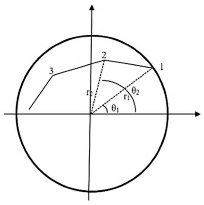
The generation of polygonal aggregates is shown in Figure 1. The origin of the coordinate system is taken as the center of the circle, and the origin is used as the polar coordinate origin. The number of sides of the aggregate, its radius, and the angles are determined to sequentially generate the coordinates of the aggregate vertices, as shown by points 1, 2, and 3 in Figure 1. Once this step is completed, the vertices are connected sequentially to form a complete shape of the aggregate. To ensure that the generated aggregate is closed, the sum of angles at each vertex should not exceed 360 degrees. This can be achieved by appropriately adjusting and limiting the calculated angles during angle calculation.

Figure 1.
Polygonal aggregate generation diagram.
2.1.2. Generating an Aggregate Library
The Valavanis Formula [30], is extensively utilized in two-dimensional aggregate research. It is employed to establish the relationship between the Fuller gradation curve and the two-dimensional gradation curve. This formula offers an effective means to parametrically describe the gradation characteristics of aggregates, enabling researchers to gain a deeper understanding and analysis of aggregate distribution. It is expressed in Equation (5) as follows:
where pc is the probability of finding an aggregate diameter D that is less than D0 at any point within the cross-section, Pk is the probability that the area of the aggregate occupies a proportion of the total area of the concrete, D is the required aggregate diameter, D0 is the aggregate gradation diameter, and Dmax is the maximum diameter of the aggregate.
Using Equation (5), the area ratio of the aggregates within each particle size range can be obtained. Then, the area of aggregates within different particle size ranges is sequentially calculated. Then, generating aggregates within a specific particle size range is stopped when the total area reaches the required value. This process yields aggregates within each particle size range, which are stored in the corresponding aggregate library.
2.1.3. Aggregate Placement
Within the designated modeling area, the aggregates are placed by calculating their size and corresponding area. During the placement process, it is essential to ensure that the aggregates are placed in an ordered manner according to the set size and to monitor the area of the aggregates placed in real time. This allows us to stop the placement process once the set total aggregate area is reached. Throughout the placement process, the boundary relationships between the aggregates need to be considered. It is crucial to ensure that the placed aggregates do not intersect or touch the existing aggregates in order to maintain their independence and integrity.
During the placement process, the positions and areas of the aggregates need to be updated in real time, and the system should monitor whether the aggregate area has reached the preset value. Once the set aggregate area is reached, the system should stop the placement process to ensure that the total aggregate area within the modeling area meets expectations.
2.2. Generation of the ITZ
After generating two-dimensional polygonal aggregates, an appropriate distance is simply extended outward based on the vertex coordinates of the polygonal aggregates to obtain the vertex coordinates of the ITZ, and then these vertices are connected. Assuming the coordinates of the aggregate are (r, θ), then the coordinates of the ITZ are (r + d, θ), where d is the thickness. Currently, there is no unified method for measuring the thickness of the ITZ. However, if the thickness is too small, it can cause mesh deformation in finite element simulations, resulting in suboptimal calculation outcomes. Ignoring its thickness during mesoscopic numerical simulations of concrete can lead to an overestimation of the mechanical properties and substantial discrepancies in damage evolution. Given the issues of mesh distortion and computational challenges, many researchers tend to slightly exaggerate the thickness of the ITZ in their mesoscopic numerical simulations.
The ITZ represents a potential site for the initiation and growth of concrete cracks, and determining an appropriate thickness of the ITZ is crucial for investigating the freeze–thaw damage mechanism in concrete. Zhou and Xu [31] found, through modeling research, that the ITZ model with added thickness performed well in the failure stage after peak strain, and the fracture morphology was more realistic. Šavija et al. [32] set the thickness of the ITZ in the mesoscopic model of corroded concrete to 1 mm and numerically simulated its cracking behavior. Wang et al. [33] and Du et al. [34] conducted mesoscopic numerical simulations of the mechanical properties of concrete specimens with an ITZ thickness of 1.0 mm, and the error compared with the experimental results did not exceed 2%. In summary, considering the stability and accuracy of the calculation, moderately increasing the thickness of the ITZ is a reasonable choice. This can effectively ensure the accuracy of the calculation results during the simulation process and avoid potential errors caused by the thickness of the transition zone being too small. Therefore, this article determines to set the thickness of the ITZ to 1.0 mm.
2.3. Generation of Two-Dimensional Mesoscopic Models
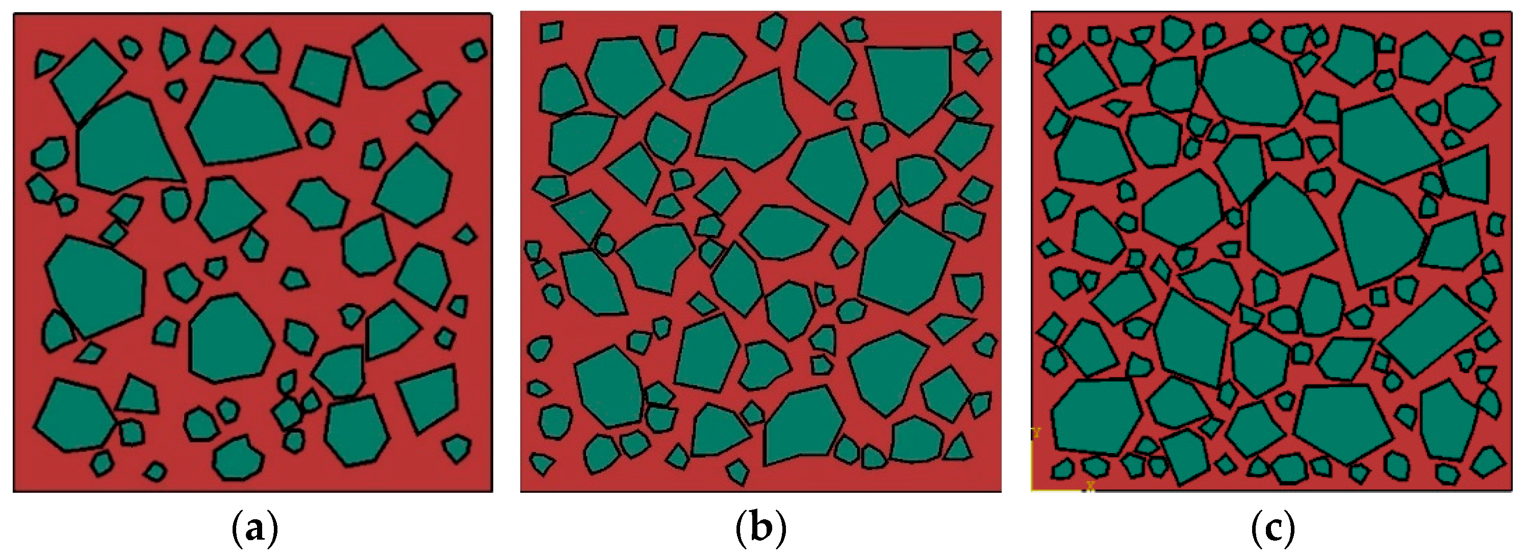
Two-dimensional mesoscopic models of concrete with randomly distributed aggregates and ITZ are generated using ABAQUS 2016 Abaqus software, as shown in Figure 2. In the generated models, the elements are square, with a side length of 100 mm × 100 mm, and the diameters of the randomly distributed aggregates range from 5 mm to 20 mm. This model allows for direct mesh generation within the software, making it convenient and efficient. The element shape primarily uses a quadrilateral advanced algorithm, with a total of 100 × 100 elements, each with an average size of 1 mm. The research results of Akcay et al. [35] indicate that, with a constant sand ratio, the elastic modulus of concrete increases as the total aggregate volume fraction increases to 40%, 49%, 58%, and 66%. Chen et al. [36] found that, for low-strength concrete, both the critical stress intensity factor and the fracture energy increase with the aggregate volume fraction (ranging from 40% to 80%), reaching their maximum value when the volume fraction is 60%. Therefore, in this study, the coarse aggregate contents of the generated meso-scale model are selected as 40%, 50%, and 60%. Three different mesoscopic models of concrete are generated based on varying aggregate contents, labeled as Figure 2 a–c, with aggregate contents of 40%, 50%, and 60%, respectively. In the models, the green polygons represent the randomly distributed aggregates, the black areas represent the ITZ, and the remaining red areas represent the mortar.

Figure 2.
Two-dimensional concrete mesoscopic models: (a) Model 1; (b) Model 2; (c) Model 3.
3. Establishment and Validation of the Concrete Freeze–Thaw Damage Model
3.1. Mechanical Performance Testing and Results
3.1.1. Specimen Fabrication
The test requires preparing cubic specimens with dimensions of 100 mm × 100 mm × 100 mm. The grading is continuous grading, and the coarse aggregate selected is crushed stone produced in Xi’an, Shaanxi Province, China, with a particle size ranging from 5 mm to 20 mm. The cement used is ordinary Portland cement produced by the Shaanxi Cement Factory, with a grade of 42.5R. The fineness modulus of the selected fine sand is 2.7. The admixtures selected are high-efficiency polycarboxylate water reducer and sodium lignosulfonate air-entraining agent. The formula for calculating the fineness modulus of the sand is given in Equation (6), as follows [37]:
where MX is the fineness modulus and A1, A2, A3, A4, A5, and A6 represent the cumulative sieve residue percentages for 4.75 mm, 2.36 mm, 1.18 mm, 0.60 mm, 0.30 mm, and 0.15 mm sieves, respectively.
The specific mix proportions are shown in Table 1.

Table 1.
Concrete mix ratio.
According to the provisions in the “GB/T 50081-2019 Standard for Test Methods of Physical and Mechanical Properties of Concrete” [38], the preparation of concrete samples is carried out as follows: First, the materials are weighed according to the mix proportions listed in Table 1, and then the ingredients are poured into a concrete mixer and mixed thoroughly. Next, the concrete mixture is poured into molds and compacted on a vibration table until the surface is covered with a layer of slurry. After molding, the specimens are demolded after 1 day of indoor curing at 20 °C and a relative humidity greater than 50% and are immediately placed in a standard curing chamber at a temperature of (20 ± 2) °C and a relative humidity of over 95% for curing. According to the “GB/T 50082-2009 Standard for Test Methods of Long-term Performance and Durability of Ordinary Concrete” [39], using the “quick-freezing method”, specimens for freeze–thaw testing should be removed from the curing location when they are 24 days old. The specimens should then be soaked in water at (20 ± 2) °C for 4 days, with the water level rising 20–30 mm above the top surface of the specimens. Freeze–thaw testing should begin when the specimens are 28 days old.
3.1.2. Test
According to the “quick-freezing method” specified in the standard [38], freeze–thaw cycling tests are conducted as follows: The concrete specimens, which have been cured for 28 days, are placed into a freeze–thaw machine for the freeze–thaw cycles. Each freeze–thaw cycle lasts between 2 and 4 h. During the freeze–thaw process, the center temperature of the specimen should be maintained at −17 ± 2 °C, while, during the thawing phase, it should be maintained at 8 ± 2 °C. A total of 150 freeze–thaw cycles are performed, with the appearance, mass, and relative dynamic elastic modulus of the samples being recorded after every 50 cycles.
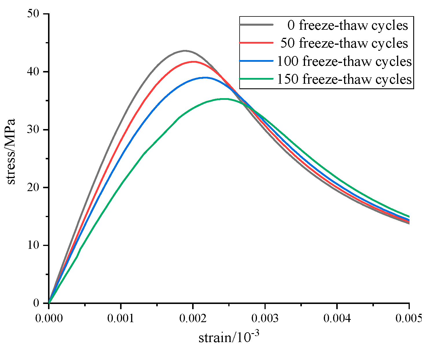
After conducting 0, 50, 100, and 150 freeze–thaw cycles, uniaxial compression tests are performed on the concrete specimens using a uniaxial compression testing machine with a loading rate of 0.4 MPa/s. The compressive strength and stress–strain curves of the concrete samples are recorded, as shown in Figure 3.

Figure 3.
Compressive stress–strain curves.
By analyzing the stress–strain curves, the elastic moduli of the concrete after 0, 50, 100, and 150 freeze–thaw cycles are found to be 32.45, 30.73, 27.75, and 22.57 GPa, respectively; the compressive strengths are 43.6, 41.71, 38.97, and 35.14 MPa, respectively; and the corresponding peak compressive strains are 0.001897, 0.002011, 0.002171, and 0.00244, respectively.
From Figure 3, it can be observed that, as the number of freeze–thaw cycles increases, the peak stress of the concrete gradually decreases, while the corresponding peak strain increases. The curves start to become progressively flatter, and the failure mode transitions from brittle to plastic. After 50 and 100 freeze–thaw cycles, the decline in the ascending segment of the curve is not very pronounced. However, after 150 freeze–thaw cycles, the decline accelerates, indicating increased damage due to the freeze–thaw cycles. As the freeze–thaw damage to the concrete increases, initial internal damage continues to accumulate and expand, the number of pores gradually increases, and the strength of the concrete decreases, making deformation more likely. This results in a change in the stress–strain relationship.
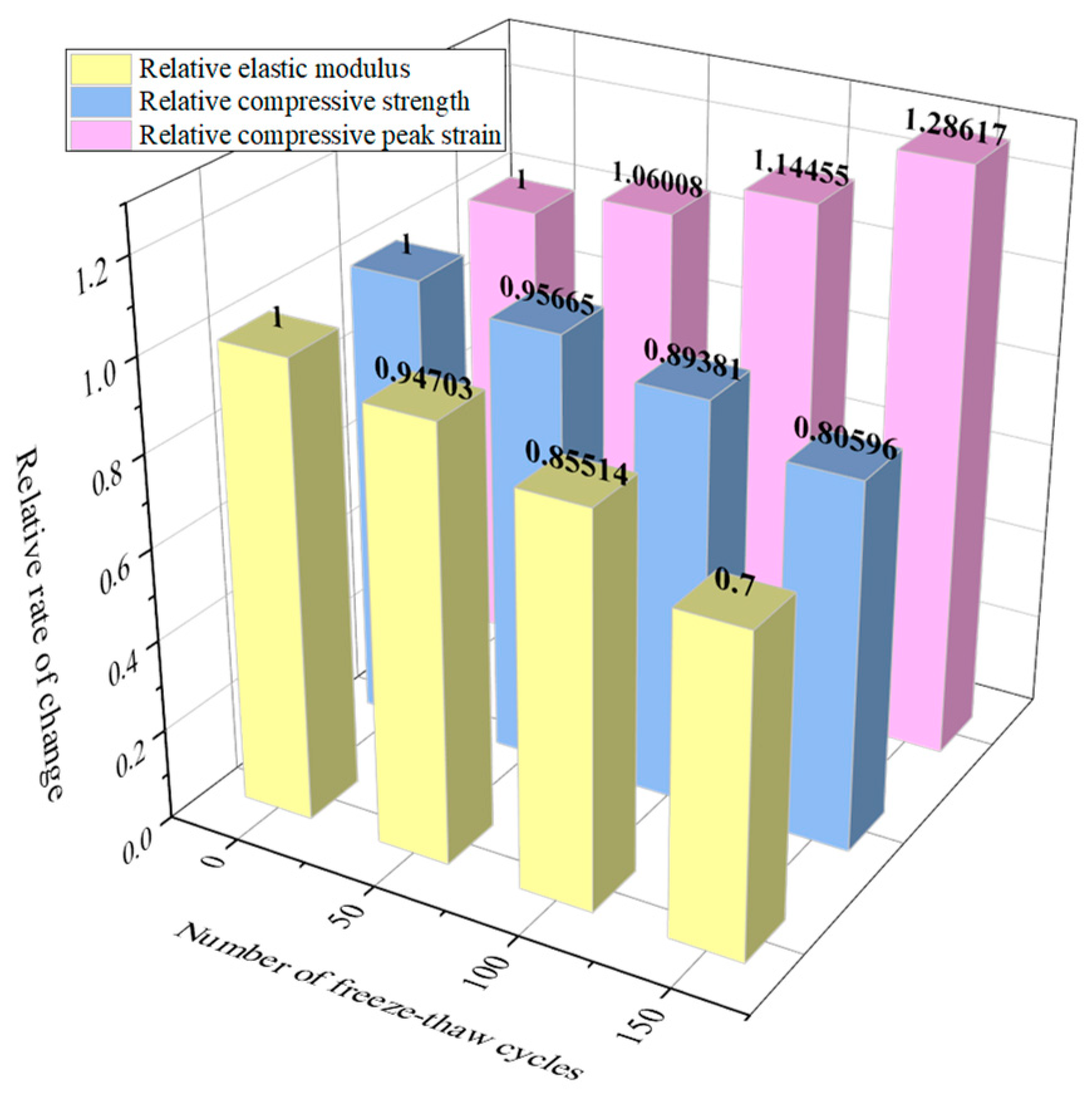
To more intuitively illustrate the changes in the mechanical performance parameters shown in Figure 3, the data from Figure 3 have been extracted and are plotted in Figure 4.

Figure 4.
Changes in the relative values of the concrete mechanical performance parameters.
From Figure 3 and Figure 4, it can be observed that the elastic modulus and compressive strength of the concrete show negative correlations with the number of freeze–thaw cycles, while the peak compressive strain shows a positive correlation. Compared to 0 freeze–thaw cycles, after 50, 100, and 150 freeze–thaw cycles, the concrete’s elastic modulus decreases by 5%, 14%, and 30%, respectively, while the compressive strength decreases by 4%, 11%, and 19%, respectively. The peak compressive strain increases by 6%, 14%, and 29%, respectively. The decrease rates in the elastic modulus and compressive strength accelerate with the increasing freeze–thaw cycles, while the increase rate in the peak compressive strain also accelerates. This is mainly due to the increase in freeze–thaw damage, which raises the porosity of the concrete, leading to a progressively looser structure and an enhanced plastic deformation capability.
3.2. Establishment of the Freeze–Thaw Damage Model
After experiencing freeze–thaw cycles, the mechanical properties of concrete gradually deteriorate, leading to structural failure and eventual collapse. Since there is no unified explanation for the freeze–thaw damage mechanism of concrete, many researchers generally adjust the relevant parameters based on the constitutive model of unfrozen concrete to establish a constitutive model for concrete after freeze–thaw damage. Freeze–thaw damage to concrete not only affects the stress–strain curve, but also deteriorates the Poisson’s ratio. By combining the relationship between the mechanical properties (elastic modulus, Poisson’s ratio, compressive strength, and tensile strength) and the number of freeze–thaw cycles fitted by Sun et al. [40], a freeze–thaw damage model based on material deterioration is proposed and applied to numerical simulation calculations.
In this section, the parameter “relative compressive strength ” is used as the fundamental quantity to establish the freeze–thaw damage model. The model incorporates the elastic modulus and compressive peak strain from the compressive stress–strain curve, as well as the tensile strength and tensile peak strain from the tensile stress–strain curve. Additionally, a correlation function between Poisson’s ratio and the relative compressive strength is utilized. These parameters are input into the Abaqus software to generate the fine-scale numerical model of freeze–thaw damage. The goal is to explore the freeze–thaw damage mechanical properties of this mesoscopic model and compare them with the mechanical performance parameters obtained from actual experiments, thereby validating the rationality of the concrete mesoscopic model. Below is the parameter correlation function for the freeze–thaw damage model.
- (1)
- Parameters of the concrete compressive stress–strain curve
According to the data collected in Section 3.1, first, the relationship between the number of freeze–thaw cycles n and the relative compressive strength is fitted. Then, the relationships are fitted between the relative elastic modulus , the relative compressive peak strain , the relative value of the ascending segment parameter , the relative value of the descending segment parameter in the compressive stress–strain curve, and the relative compressive strength , respectively, denoted as Equations (7)–(11). The relative values of the ascending segment parameters and the descending segment parameters are shown in Table 2.
where is the parameter of the n times ascent of the freeze–thaw cycle, is the parameter of unfreezing-thawing ascent, is the peak compressive strain value of the concrete during the freeze–thaw cycle n times, is the peak compressive strain value of the unfrozen and thawed concrete, is the elastic modulus of the concrete for n times of the freeze–thaw cycle, is the elastic modulus value of the unfrozen and thawed concrete, is the compressive strength of the concrete during the freeze–thaw cycle n times, is the compressive strength of the unfrozen and thawed concrete, is the parameter of the n times descending stage of the freeze–thaw cycle, and is the unfreezing-thawing descending stage parameter.
Table 2.
Parameter values of the ascending and descending sections under each number of freeze–thaw cycles.
- (2)
- Parameters of tensile stress–strain curve of concrete
The relative tensile strength and the relative tensile peak strain , with respect to the relative compressive strength , were denoted by Cao [41] and Shang et al. [42]. Consequently, the relationship between the descending segment parameter and the relative compressive strength can be obtained. These relationships are denoted as Equations (12)–(14).
- (i)
- Relative tensile strength
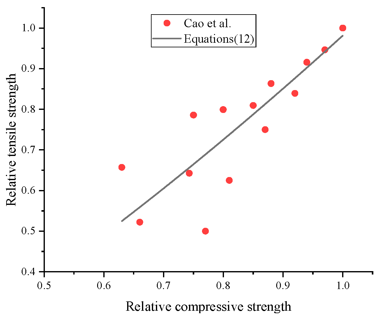
Based on the experimental data from Cao et al. [41], the relationship between the relative tensile strength and the relative compressive strength is fitted, as shown in Figure 5. The fitted formula is given in Equation (12).

Figure 5.
The relationship between the relative tensile strength and relative compressive strength [41].
- (ii)
- Relative peak tensile strain
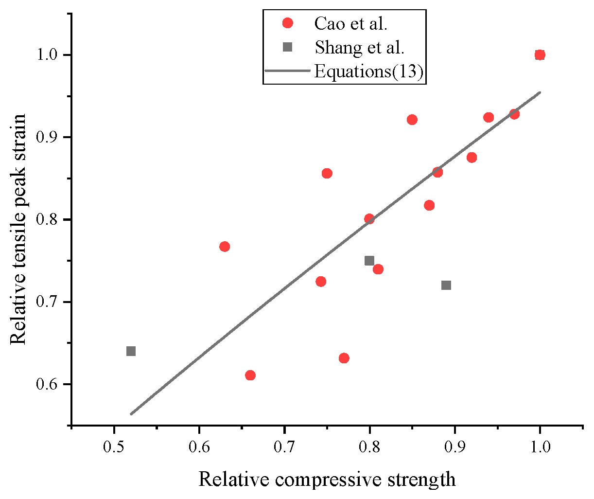
Based on the experimental data from Cao et al. [41] and Shang et al. [42], the fitting process for the relationship between the relative peak tensile strain and the relative compressive strength is shown in Figure 6. The corresponding formula is given in Equation (13).

Figure 6.
The relationship between the relative tensile peak strain and relative compressive strength [41,42].
- (iii)
- Decline segment parameter ratio
The decline segment parameter is . The relationship between the decline segment parameter ratio and the relative compressive strength is given in Equation (14) below, as follows:
where is the tensile strength of freezing and thawing n times, is the tensile strength of the unfrozen and thawed concrete, is the peak tensile strain of the freeze–thaw n times, is the peak tensile strain of the concrete before the freeze–thaw cycle, is the descending stage parameter after n freeze–thaw cycles, and is the parameter of the descending section before the freeze–thaw cycle of the concrete.
- (3)
- Relative Poisson’s ratios
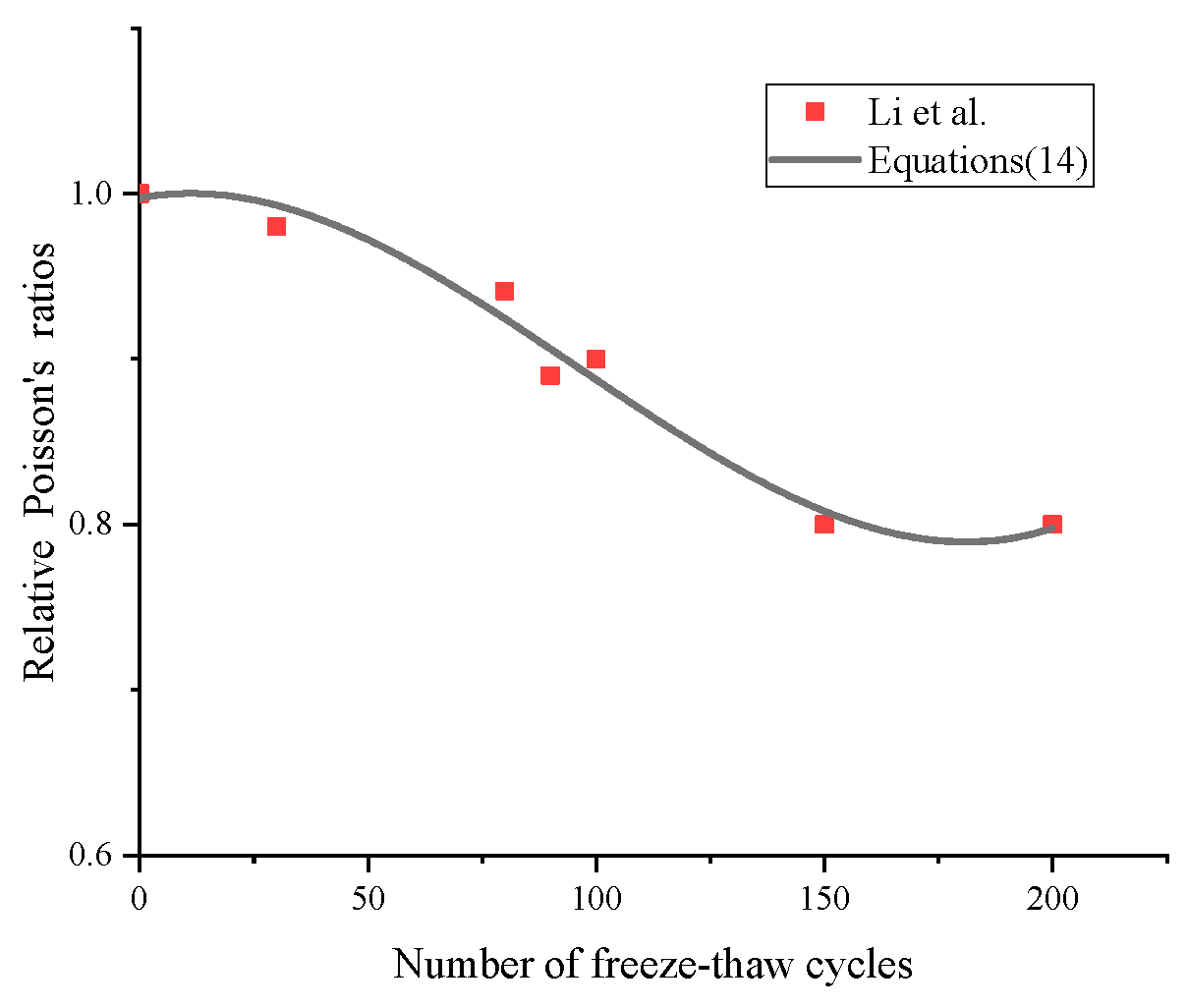
Poisson’s ratio is an indicator of the lateral deformation of concrete. Under the action of freeze–thaw cycles, the material’s Poisson’s ratio will also undergo corresponding changes. Li et al. [43] studied the variation of Poisson’s ratio of materials subjected to freeze–thaw cycles. The fitting process is shown in Figure 7, and the relationship is shown in Equation (15).
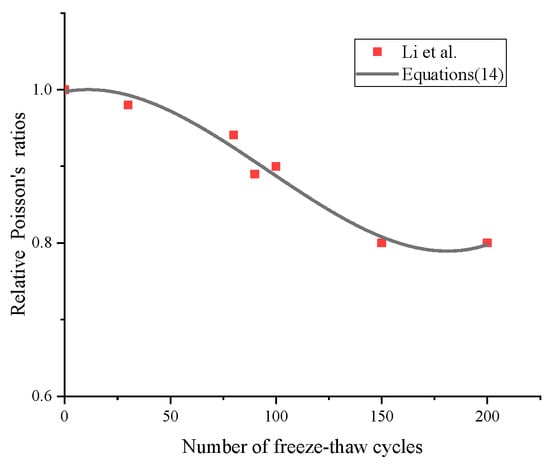
Figure 7.
The relationship between the relative Poisson’s ratio and number of freeze–thaw cycles [43].
Substituting Equation (15) into Equation (7) allows for the fitting of the relationship for the Poisson’s ratio parameter in the freeze–thaw damage model, as shown in Equation (16), as follows:
where is the Poisson’s ratio of the concrete for n freeze–thaw cycles and is the Poisson’s ratio of the unfrozen and thawed concrete.
In this section, the relationships between the relative compressive strength, the relative tensile–compressive strength, the relative elastic modulus, and the relative tensile–compressive peak strain were fitted, establishing the freeze–thaw damage model for concrete.
3.3. Validation of Fine-Scale Numerical Simulation of the Freeze–Thaw Damage Model
Because the constitutive model of coarse aggregates is linear elastic and their elastic modulus is relatively high, making them less susceptible to plastic deformation, and the freeze–thaw damage of concrete is mainly caused by the initiation and gradual propagation of microcracks in the mortar and ITZ under freeze–thaw cycles, macroscopic cracks and concrete damage occur. Therefore, this study does not consider the freeze–thaw damage of coarse aggregates and applies the concrete freeze–thaw damage model to the freeze–thaw damage of mortar and ITZ.
The method to validate the rationality of the freeze–thaw damage model is to first calculate the parameter values required for the concrete model under different freeze–thaw cycles in the ABAQUS 2016 Then, fine-scale numerical simulation of concrete uniaxial compression is conducted, and then the stress–strain curve, compressive strength, compressive peak strain, and elastic modulus of concrete are obtained and compared with the experimental data.
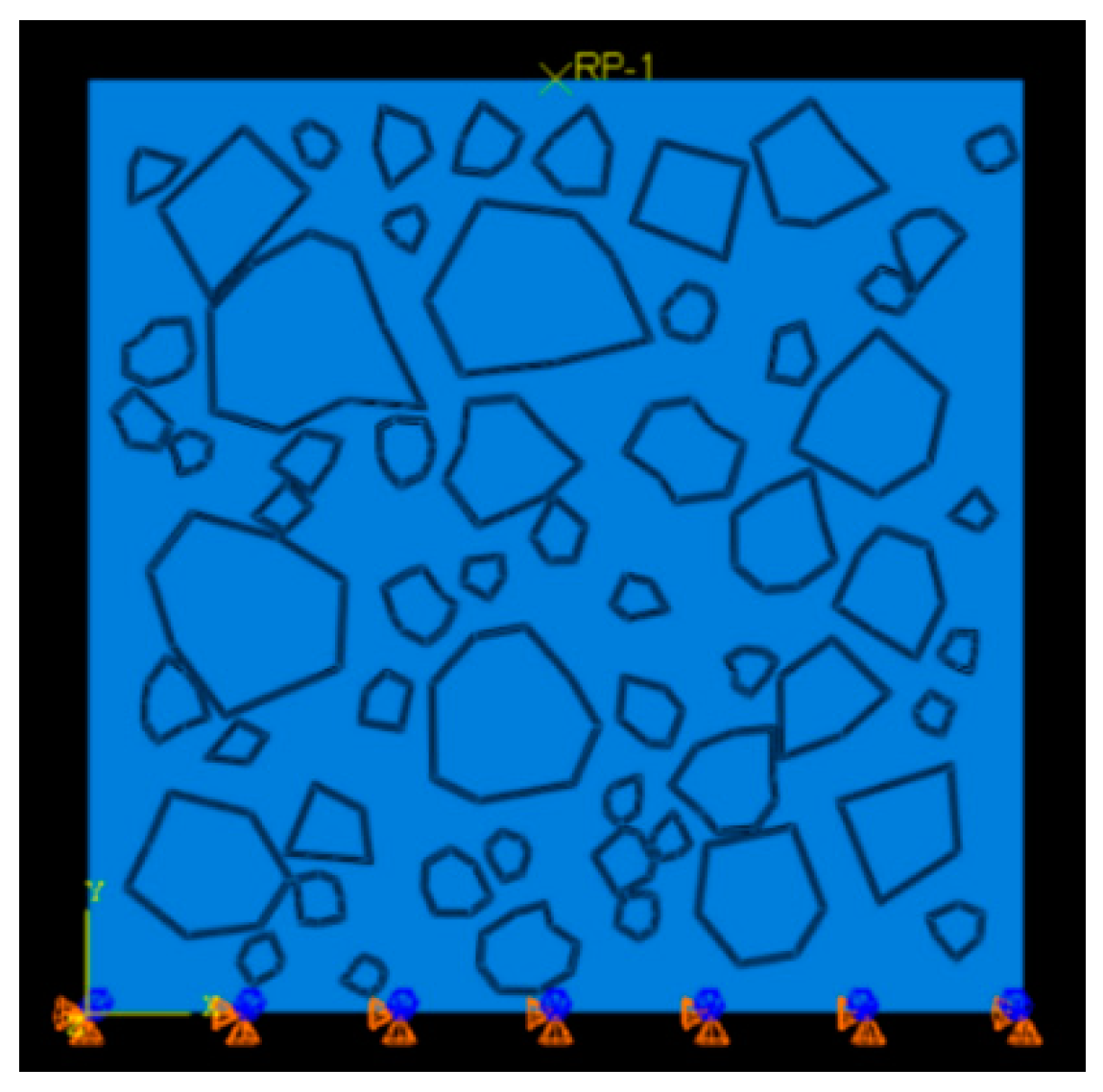
The two-dimensional, fine-scale model of concrete with 40% coarse aggregate content (denoted as Figure 2a) is chosen for rationality verification. First, the parameters of the mortar and ITZ under each freeze–thaw cycle are input into the model generated in the ABAQUS 2016. Then, numerical simulations are conducted on uniaxial compression tests on the fine-scale model to obtain the load–displacement curves under 0, 50, 100, and 150 freeze–thaw cycles, and, thus, the stress–strain curves are obtained. The numerical simulation method for the uniaxial compression of concrete involves fixing the bottom edge of the concrete specimen with free boundaries on the sides. A reference point, RP-1, is selected at the center of the top edge of the specimen for coupling. A downward load is applied to the reference point in a displacement-controlled manner, as shown in Figure 8. The seven orange and blue markers at the bottom of Figure 8 represent the fixed points of the concrete specimen
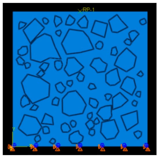
Figure 8.
Schematic diagram of the numerical simulation of concrete uniaxial compression.
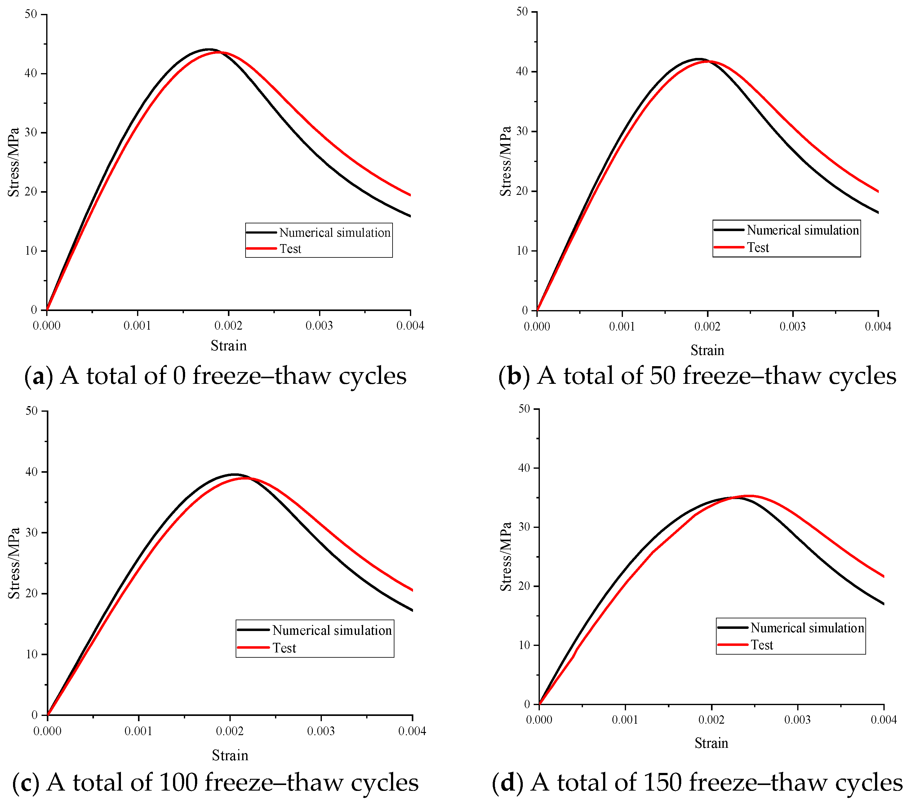
From the stress–strain curves, the compressive strength, compressive peak strain, and elastic modulus of the concrete model are extracted and compared with the curves and experimental results obtained in Section 3.1. A comparison between the experimental results and numerical simulation stress–strain curves under different freeze–thaw cycles is shown in Figure 9.
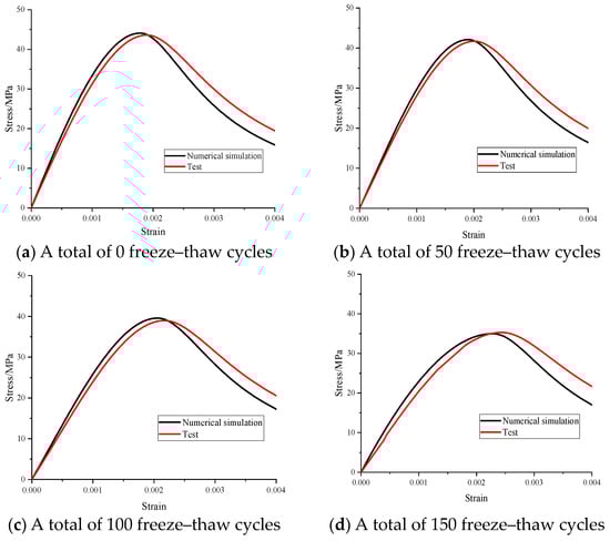
Figure 9.
Comparison of the experimental and numerical stress–strain curves under various freeze–thaw cycles.
According to the analysis of Figure 9, the linear segments and the ascending segments of the experimental and numerical simulation stress–strain curves before reaching the maximum stress fit well under 0, 50, and 100 freeze–thaw cycles. However, there are slight differences in the descending segments after reaching the maximum stress, which may be attributed to discrepancies between the values of meso-scale parameters of the ITZ, the aggregates, and the actual material. Under 150 freeze–thaw cycles, the differences in the slopes of the linear segment before reaching the maximum stresses and the maximum stresses become larger. The main reason for the increased differences in curve fitting may be that the Abaqus software cannot simulate the interfacial contact between the aggregates, the mortar, and the ITZ in concrete well. However, the stress–strain curves obtained from the numerical simulation of the uniaxial compression tests fit well with the experimental curves.
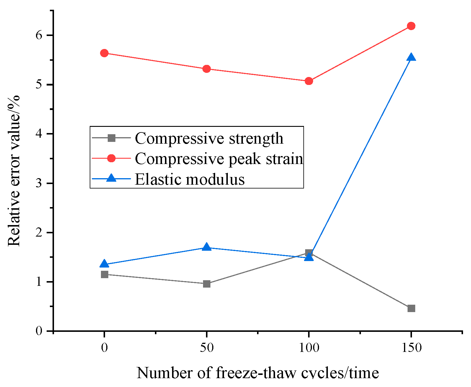
To visually compare the numerical simulation results with the experimental data, a statistical analysis of the compressive strength, compressive peak strain, and elastic modulus of the concrete after the freeze–thaw cycles was conducted. The key performance parameters of the concrete under different freeze–thaw cycle numbers are as follows: for 0 cycles, the elastic modulus is 32.98 GPa, the compressive strength is 44.1 MPa, and the compressive peak strain is 0.00179; for 50 cycles, the elastic modulus is 31.25 GPa, the compressive strength is 42.11 MPa, and the compressive peak strain is 0.001904; for 100 cycles, the elastic modulus is 28.16 GPa, the compressive strength is 39.59 MPa, and the compressive peak strain is 0.002061; and, for 150 cycles, the elastic modulus is 23.82 GPa, the compressive strength is 34.98 MPa, and the compressive peak strain is 0.002289. The error analysis of the numerical simulation results compared to the experimental data yielded relative errors, as shown in Figure 10.
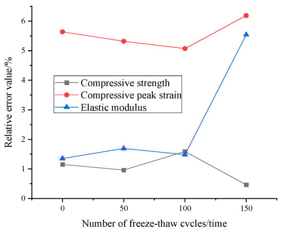
Figure 10.
Relative errors of the mechanical properties in the concrete experiment and numerical simulation.
An analysis of Figure 10 reveals that the relative errors of concrete compressive strength under 0, 50, 100, and 150 freeze–thaw cycles are 1.15%, 0.96%, 1.59%, and 0.46%, respectively. The relative errors of compressive peak strain are 5.64%, 5.32%, 5.07%, and 6.19%, respectively. The relative errors of the elastic modulus are 1.35%, 1.69%, 1.48%, and 5.54%, respectively. The relative errors of various mechanical performance parameters between the experimental and the numerical simulation results are all below 7%, which sufficiently validates the rationality of this two-dimensional freeze–thaw damage mesoscopic model for concrete.
4. Parametric Study of Fine-Scale Numerical Simulation of Concrete Freeze–Thaw Damage
This section investigates the evolution of the mechanical properties of freeze–thaw-damaged concrete from a mesoscopic perspective. Building upon the validation of the freeze–thaw damage model, this study explores the influences of mesoscopic parameters on the mechanical properties of freeze–thaw-damaged concrete by altering the ratios of parameters in the ITZ and the content of coarse aggregates in the concrete. Uniaxial compression fine-scale numerical simulations are conducted to explore the impact of the mesoscopic parameters on the mechanical properties of freeze–thaw-damaged concrete.
4.1. Effect of Changes in the Ratio of Concrete Mechanical Properties at the ITZ
The ITZ refers to the thin layer between the aggregate and the cement paste in concrete. It is an independent phase within the concrete material and is the weakest link. When concrete is subjected to external loads, microcracks first appear at the ITZ and gradually extend into the cement paste, eventually leading to the failure of the concrete structure. The structure of the ITZ is relatively complex, making it difficult to study its mechanical properties independently. It is typically assumed that the structure of the ITZ is similar to that of the cement paste, and its constitutive model is also taken as an elastoplastic damage model. Consequently, many researchers use the same ratios of the ITZ’s main mechanical property parameters (compressive strength, tensile strength, and elastic modulus) as those of the cement paste, with these ratios generally ranging from 0.7 to 0.9 [44,45,46]. Therefore, in this section, without altering the mechanical property parameters of the aggregates and mortar, we vary the ratios of the mechanical property parameters (elastic modulus and compressive strength) between the ITZ and the mortar to be 0.7, 0.8, and 0.9, respectively. This allows for investigating the influence of changes in the ratios of parameters in the ITZ on the mechanical properties of the freeze–thaw-damaged concrete. Therefore, the two-dimensional freeze–thaw damage mesoscopic model of the concrete (Figure 2a) is retained.
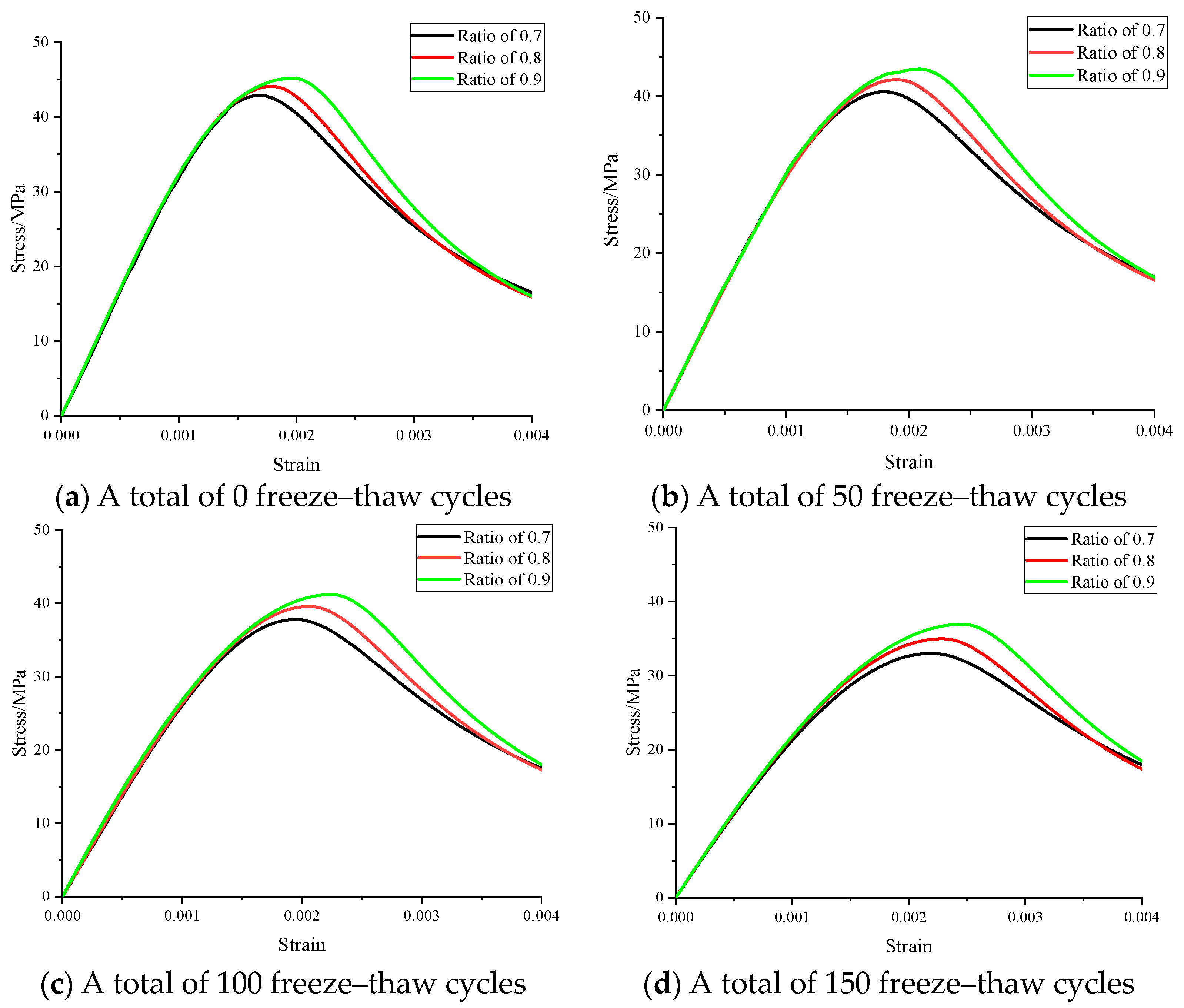
Numerical simulation uniaxial compression tests are conducted on the fine-scale model. Figure 11 presents the stress–strain curves under different freeze–thaw cycle numbers and different ratios of ITZ.

Figure 11.
The stress–strain curves examined across different freeze–thaw cycles, with variations in the interfacial transition zone ratios taken into account.
By extracting and analyzing the stress–strain curves from Figure 11, we can obtain the relative changes in the mechanical performance parameters. The results are summarized in Table 3.
Table 3.
The relative changes in the mechanical properties analyzed under various freeze–thaw cycles and interfacial transition zone ratios.
From Table 3, it is evident that, with the increase in the ratio of ITZ parameters, the compressive strength of concrete increases, indicating an enhancement in frost resistance. When the ITZ parameter ratios are 0.8 and 0.9, compared to the ratio of 0.7, the compressive strength at 0 freeze–thaw cycles increases by 2.77% and 5.41%, respectively; at 50 cycles, it increases by 3.82% and 7.13%, respectively; at 100 cycles, it increases by 4.71% and 8.99%, respectively; and, at 150 cycles, it increases by 5.97% and 11.91%, respectively. This indicates that increasing the ITZ parameter ratio improves its mechanical properties and enhances the frost resistance of concrete.
According to the data in Table 3, when the parameter ratio is 0.7, compared to 0 freeze–thaw cycles, the elastic modulus decreases by 5.60%, 15.23%, and 28.72% after 50, 100, and 150 freeze–thaw cycles, respectively; the compressive strength decreases by 5.41%, 11.82%, and 23.02%, respectively; and the compressive peak strain increases by 6.95%, 15.56%, and 30.40%, respectively. For a parameter ratio of 0.8, the corresponding elastic modulus decreases by 5.23%, 14.63%, and 27.77%, respectively; the compressive strength decreases by 4.51%, 10.23%, and 20.68%, respectively; and the compressive peak strain increases by 6.37%, 15.14%, and 27.88%, respectively. For a parameter ratio of 0.9, compared to 0 freeze–thaw cycles, the elastic modulus decreases by 4.94%, 13.81%, and 27.05% after 50, 100, and 150 freeze–thaw cycles, respectively; the compressive strength decreases by 3.87%, 8.83%, and 18.27%, respectively; and the compressive peak strain increases by 5.88%, 13.89%, and 24.73%, respectively.
An analysis of Figure 11 and Table 3 reveals that, with the increase in the ratio of ITZ, the variations in the compressive strength and compressive peak strain of concrete gradually decrease, while the fluctuations in the elastic modulus are relatively small. This suggests that increasing the ratio of the ITZ parameters helps to enhance the mechanical properties of concrete, especially in terms of further improving the compressive strength and compressive peak strain. However, the increase in the ratio of ITZ parameters has a relatively minor effect on the elastic modulus of concrete, which can be almost neglected. Under the same ratios of ITZ parameters, as the number of freeze–thaw cycles increases, the rates of change in various mechanical properties of concrete gradually accelerate, indicating gradual weakening trends in the concrete performance as the number of freeze–thaw cycles increases.
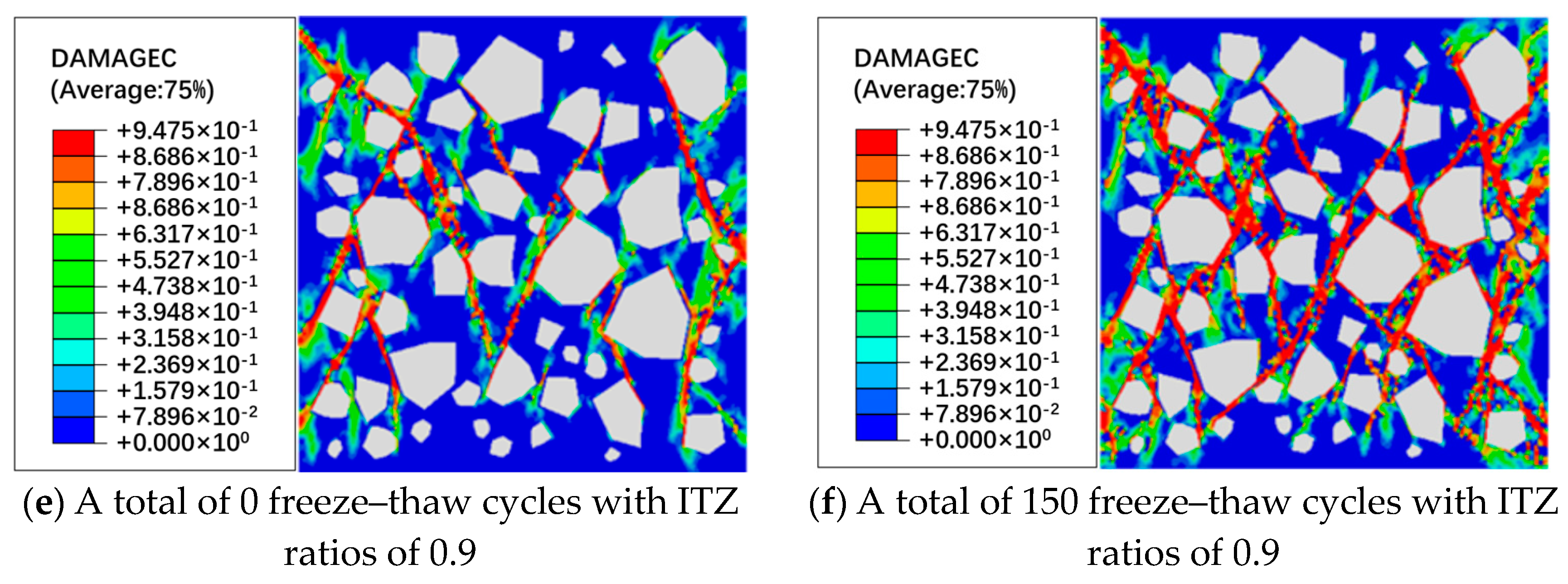
In this study, the development of internal cracks in concrete after 150 freeze–thaw cycles under different scenarios with ITZ ratios of 0.7, 0.8, and 0.9 was investigated. The microcrack distributions in the concrete at peak stress are illustrated in Figure 12.
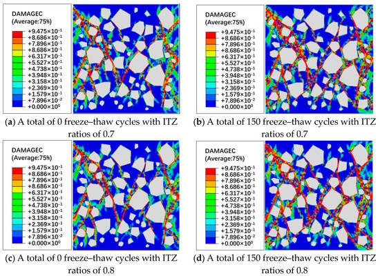
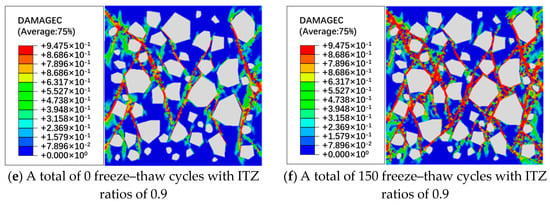
Figure 12.
Mesoscopic damage contours of concrete under different interfacial transition zone ratios.
An analysis of Figure 12 reveals that, compared to 0 freeze–thaw cycles, after 150 freeze–thaw cycles, concrete exhibits X-shaped internal cracks that propagate outward, with a significant increase in damage and even the occurrence of through cracks under compression. Despite the observed influence of the ratio of ITZ parameters on the mechanical properties of concrete, as summarized from the data, the variations in the ratios of the ITZ parameters do not affect the mode of internal crack development in concrete, as evidenced by the observed pattern of internal crack propagation.
4.2. Effect of Changes in the Coarse Aggregate Content Variation on Concrete Mechanical Properties
The distributions of coarse aggregates in concrete are quite random, accounting for relatively high proportions, generally ranging from 40% to 60% of the concrete volume, which has a certain impact on the mechanical properties of freeze–thaw-damaged concrete. Therefore, in this section, without altering the mechanical properties of the mesoscopic materials, three concrete mesoscopic models with coarse aggregate contents of 40%, 50%, and 60% were selected in order to explore the influence of coarse aggregate content on the mechanical properties of freeze–thaw-damaged concrete.
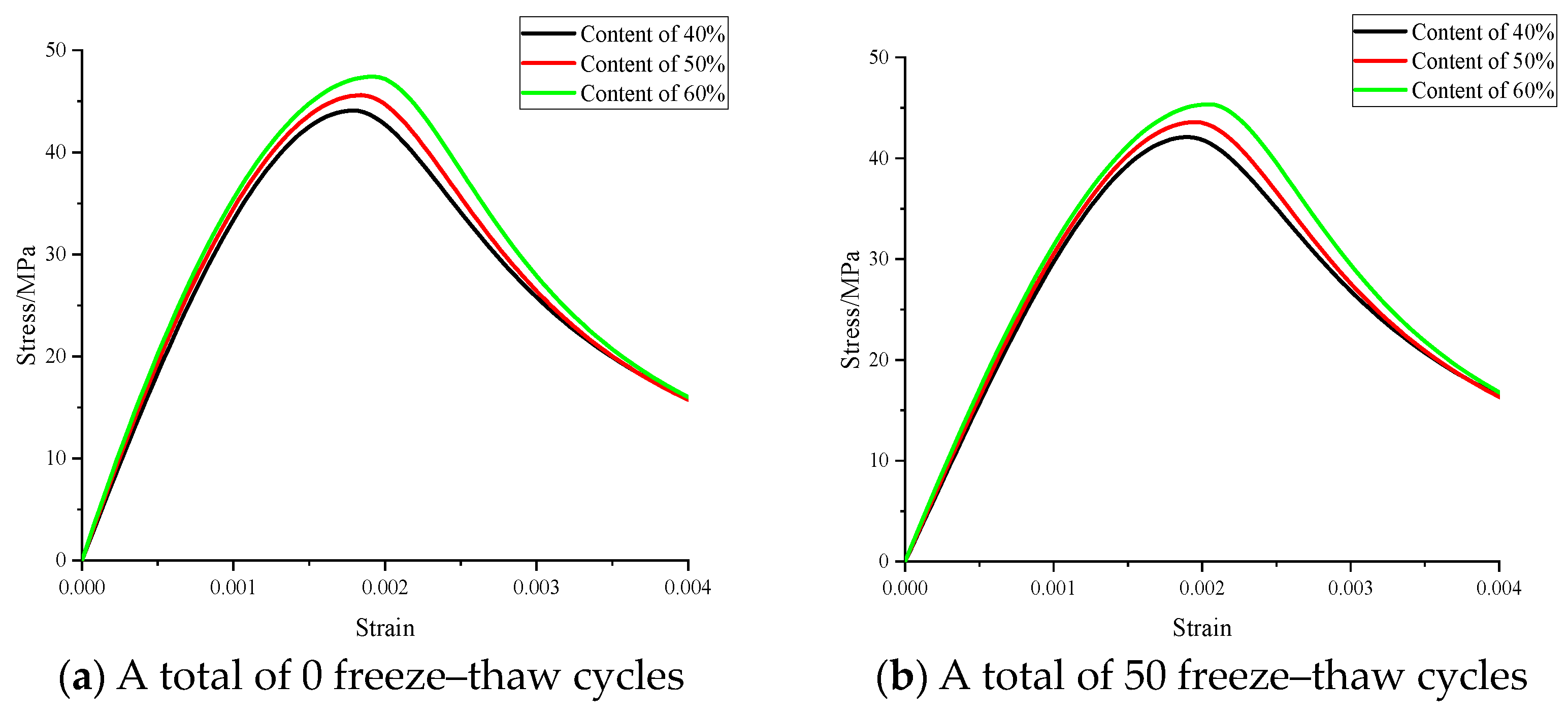
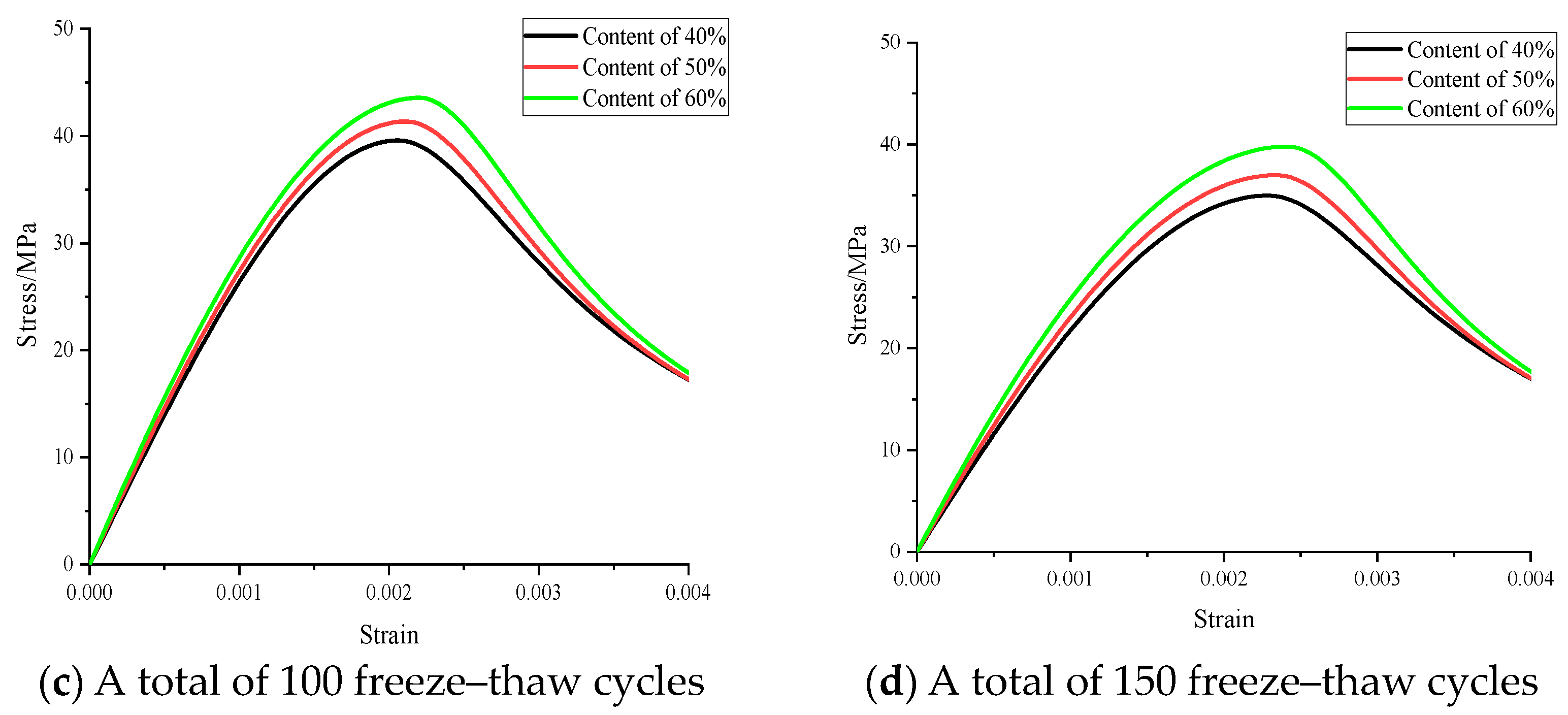
Numerical simulations of uniaxial compression tests were conducted on the mesoscopic models to obtain the stress–strain curves under different freeze–thaw cycles and different coarse aggregate contents, as shown in Figure 13.
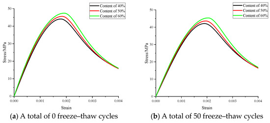
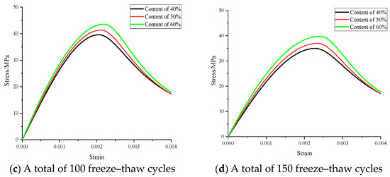
Figure 13.
Stress–strain curves observed across diverse freeze–thaw cycles and varying levels of coarse aggregate content.
Extracting and summarizing the mechanical performance parameters from the stress–strain curves in Figure 13, the relative variations of various mechanical performance parameters can be obtained, as shown in Table 4.
Table 4.
The relative fluctuations in mechanical properties in relation to different freeze–thaw cycles and coarse aggregate contents.
According to Table 4, it can be observed that, with an increase in coarse aggregate content, the compressive strength of concrete increases, leading to improved frost resistance. When the coarse aggregate contents are 50% and 60%, compared to concrete with 40% coarse aggregate content, the compressive strengths of concrete without freeze–thaw cycles increase by 3.40% and 7.53%, respectively. After 50 cycles, they increase by 3.51% and 7.72%, respectively; after 100 cycles, they increase by 4.47% and 10.08%, respectively; and, after 150 cycles, they increase by 5.75% and 13.75%, respectively. This indicates that increasing the coarse aggregate content reduces the amount of mortar susceptible to freeze–thaw damage and helps to hinder crack propagation. Although there is an increase in the number of weaker ITZs, the overall elastic modulus of the concrete increases, leading to higher strength and improved freeze–thaw resistance.
According to Table 4, for a coarse aggregate content of 40%, compared to no freeze–thaw cycles, after 50, 100, and 150 freeze–thaw cycles, the elastic modulus decreases by 5.23%, 14.63%, and 27.77%, respectively; the compressive strength decreases by 4.51%, 10.23%, and 20.68%, respectively; and the peak compressive strain increases by 6.37%, 15.14%, and 27.88%, respectively. For a coarse aggregate content of 50%, compared to no freeze–thaw cycles, after 50, 100, and 150 freeze–thaw cycles, the elastic modulus decreases by 5.07%, 14.17%, and 25.58%, respectively; the compressive strength decreases by 4.41%, 9.30%, and 18.89%, respectively; and the peak compressive strain increases by 6.13%, 14.70%, and 27.24%, respectively. For a coarse aggregate content of 60%, compared to no freeze–thaw cycles, after 50, 100, and 150 freeze–thaw cycles, the elastic modulus decreases by 4.88%, 13.06%, and 23.13%, respectively; the compressive strength decreases by 4.34%, 8.10%, and 16.09%, respectively; and the peak compressive strain increases by 6.11%, 14.34%, and 25.51%.
An analysis of Figure 13 and Table 4 reveals that, as the coarse aggregate content increases, the changes in the compressive strength, elastic modulus, and compressive peak strain decrease, but the reductions are relatively small. By increasing the coarse aggregate content, the mechanical properties of concrete are effectively improved, indicating that adjusting the coarse aggregate content reasonably in the concrete mix design can improve the overall material performance. Compared to 0 freeze–thaw cycles, the rates of change in various mechanical properties of concrete accelerate with an increase in the number of freeze–thaw cycles. This clearly demonstrates the rapid deterioration of concrete durability with an increase in the amount of freeze–thaw cycles.
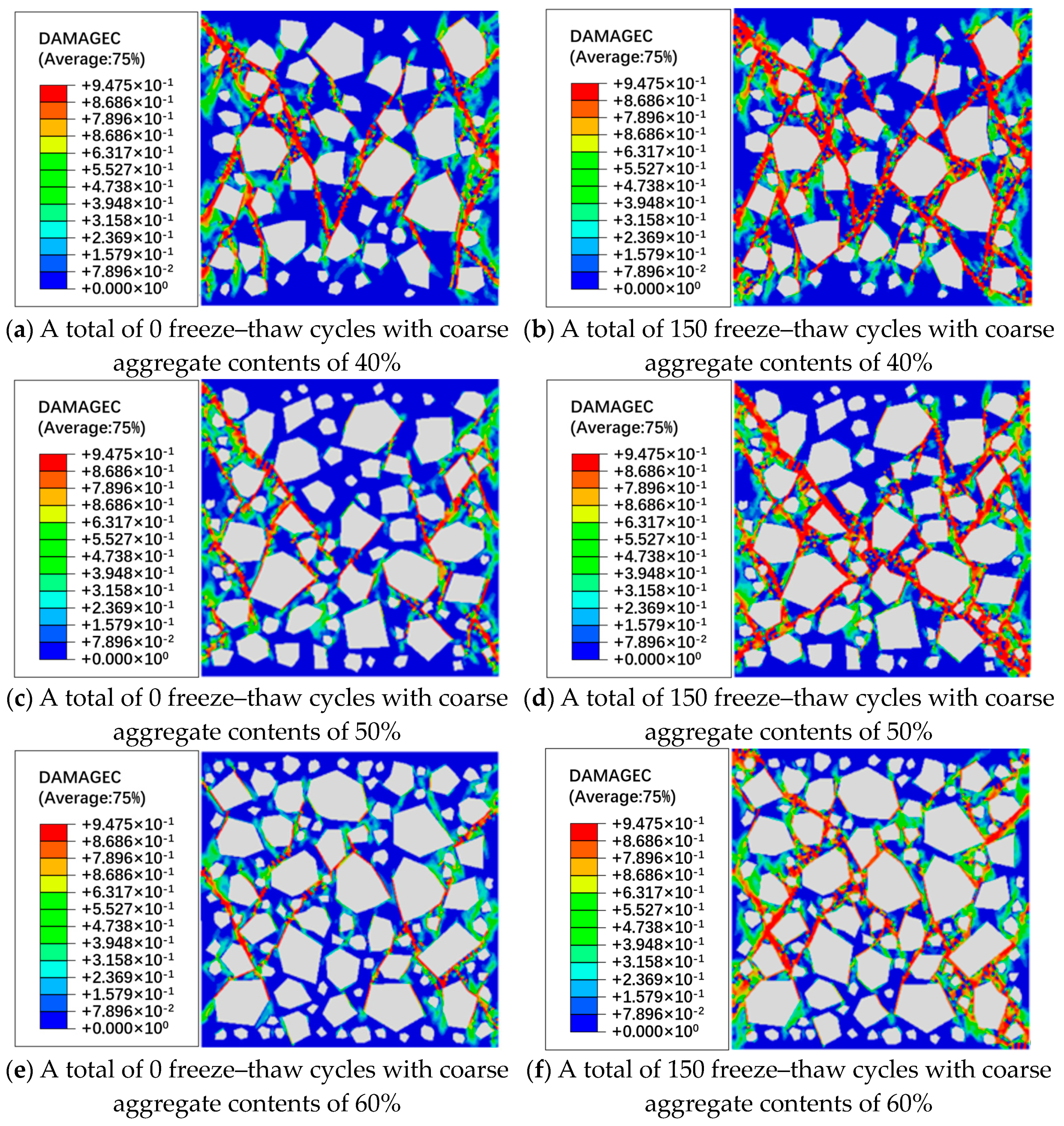
This section also investigates the micro-damage contours of concrete at the maximum stress under 150 freeze–thaw cycles with coarse aggregate contents of 40%, 50%, and 60%, as shown in Figure 14.
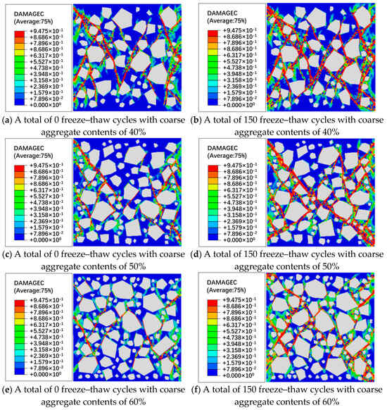
Figure 14.
Mesoscopic damage contours of concrete under different coarse aggregate contents.
Based on the analysis of Figure 14, it can be inferred that, after 150 freeze–thaw cycles, regardless of variations in coarse aggregate content, concrete exhibits a tendency for internal cracks to expand in an X-shaped pattern towards the surroundings when subjected to pressure. However, with an increase in the coarse aggregate content in concrete, the coarse aggregates can better encapsulate the mortar, leading to a greater number of development paths for internal cracks in concrete. These additional cracks can effectively dissipate the externally applied pressure, thereby slowing down the rate of crack propagation. Although more microcracks may be generated, their presence contributes to enhancing the strength and frost resistance of concrete. Therefore, increasing the content of coarse aggregates in concrete has a positive effect on improving its performance.
5. Conclusions
The concrete freeze–thaw damage model was applied to the two-dimensional mesoscopic model of concrete with random aggregates, and a fitting analysis was conducted on the experimental data and previous data using the “relative compressive strength” as a variable. This process established the concrete freeze–thaw damage model, and numerical simulations of the uniaxial compression tests were performed to validate the rationality of the damage model. Finally, by changing the parameters of the ITZ and the coarse aggregate content, mesoscopic simulations of freeze–thaw-damaged concrete under uniaxial compression were conducted. The conclusions are drawn as follows:
- (1)
- Generating polygonal random aggregates based on circular aggregates is simple and can effectively reduce the complexity of edge-to-edge determination. By extending to a certain distance from the vertices of the polygonal aggregates, the ITZ can be generated. This method can not only meet the required aggregate packing density, but also facilitate grid division directly in the Abaqus software.
- (2)
- The numerical simulation results of the freeze–thaw damage model fit well with the experimental data for the stress–strain curves, with the relative errors of all mechanical performance parameters being below 7%. This indicates that the model can accurately simulate the mechanical properties of the mesoscopic concrete after freeze–thaw damage, further confirming the reliability and rationality of the freeze–thaw damage mesoscopic model.
- (3)
- Higher ITZ parameter ratios improve the mechanical properties of the ITZ in concrete, leading to increased compressive strength and peak compressive strain, but they have almost no impact on the elastic modulus. Compared to the ratios of 0.7 and 0.8, concrete with a ratio of 0.9 experiences slower reduction rates in compressive strength and elastic modulus and a slower increase rate in peak compressive strain after undergoing freeze–thaw cycles. Increasing the ITZ parameter ratio enhances the mechanical properties of the ITZ and strengthens the concrete’s resistance to freezing.
- (4)
- Concrete with a higher coarse aggregate content exhibits a higher compressive strength, peak compressive strain, and elastic modulus. Compared to that with contents of 40% and 50%, concrete with a content of 60% experiences slower reduction rates in compressive strength and elastic modulus and a slower increase rate in peak compressive strain after undergoing freeze–thaw cycles, indicating that increasing the coarse aggregate content enhances the concrete’s strength and frost resistance.
Author Contributions
Conceptualization, R.W.; Data curation, J.H., H.Z., and Y.J.; Formal analysis, N.Y. and G.L.; Investigation, J.L.; Methodology, Y.L. (Yang Li); Resources, R.J. and Y.L. (Yanxiong Liu); Supervision, Y.L. (Yang Li) and J.L.; Validation, Y.L. (Yunhui Liu) and Y.L. (Yang Li); Writing—original draft, Y.L. (Yunhui Liu); Writing—review and editing, Y.L. (Yunhui Liu); Funding acquisition, G.L. and Y.L. (Yang Li). All authors have read and agreed to the published version of the manuscript.
Funding
This research was funded by the National Natural Science Foundation of China (Grant No. 52379133) and China Postdoctoral Science Foundation (Program No. 2020M683687XB).
Data Availability Statement
The original contributions presented in the study are included in the article, further inquiries can be directed to the corresponding author.
Conflicts of Interest
Authors Jun Liu, Ruibao Jin and Jing Hu were employed by the company Henan Jiaotou Jiaozheng Expressway Co., Ltd. Authors Hekuan Zhou, Yaofei Jia and Yanxiong Liu were employed by the company Henan Province Highway Engineering Bureau Group Co., Ltd. The remaining authors declare that the research was conducted in the absence of any commercial or financial relationships that could be construed as a potential conflict of interest.
References
- Bahrami, N.; Zohrabi, M.; Mahmoudy, S.A.; Akbari, M. Optimum recycled concrete aggregate and micro-silica content in self-compacting concrete: Rheological, mechanical and microstructural properties. J. Build. Eng. 2020, 31, 101361. [Google Scholar] [CrossRef]
- Li, T.; Wang, S.L.; Xu, F. Study of the basic mechanical properties and degradation mechanism of recycled concrete with tailings before and after carbonation. J. Clean. Prod. 2020, 259, 120923. [Google Scholar] [CrossRef]
- Ren, R.; Qi, L.J.; Xue, J.Y.; Zhang, X. Cyclic bond property of steel reinforced recycled concrete (SRRC) composite structure. Constr. Build. Mater. 2020, 245, 118435. [Google Scholar] [CrossRef]
- Zhang, M.J.; Yu, H.F.; Zhang, J.H.; Chen, B.Y.; Ma, H.Y.; Gong, X.; Guo, J.B.; Yu, W.M.; Li, L.Y. Finite element analysis of stress–strain relationship and failure pattern of concrete under uniaxial compression considering freeze–thaw action. Eng. Fract. Mech. 2023, 290, 109520. [Google Scholar] [CrossRef]
- Liu, S.; Liu, H.D.; Liu, H.N.; Xia, Z.G.; Zhao, Y.W.; Zhai, J.Y. Numerical simulation of mesomechanical properties of limestone containing dissolved hole and persistent joint. Theor. Appl. Fract. Mech. 2022, 122, 103572. [Google Scholar] [CrossRef]
- Liu, M.M.; Wang, F.T. Numerical simulation of influence of coarse aggregate crushing on mechanical properties of concrete under uniaxial compression. Constr. Build. Mater. 2022, 342, 128081. [Google Scholar] [CrossRef]
- Chatterji, S. Aspects of freezing process in porous material-water system: Part 2. Freezing and properties of frozen porous materials. Cem. Concr. Res. 1999, 29, 781–784. [Google Scholar] [CrossRef]
- Deng, X.H.; Gao, X.Y.; Wang, R.; Gao, M.X.; Yan, X.X.; Cao, W.P.; Liu, J.T. Investigation of microstructural damage in air-entrained recycled concrete under a freeze–thaw environment. Constr. Build. Mater. 2021, 268, 121219. [Google Scholar] [CrossRef]
- Luo, Q.; Liu, D.; Qiao, P.; Feng, Q.; Sun, L. Microstructural damage characterization of concrete under freeze-thaw action. Int. J. Damage Mech. 2018, 27, 1551–1568. [Google Scholar]
- He, R.; Zheng, S.N.; Vincent, J.L.G.; Wang, Z.D.; Fang, J.H.; Shao, Y. Damage mechanism and interfacial transition zone characteristics of concrete under sulfate erosion and Dry-Wet cycles. Constr. Build. Mater. 2020, 255, 119340. [Google Scholar] [CrossRef]
- Golewski, G.L. Physical characteristics of concrete, essential in design of fracture-resistant, dynamically loaded reinforced concrete structures. Mater. Des. Process. Commun. 2019, 1, e82. [Google Scholar] [CrossRef]
- Ippei, M.; Hiroshi, S.; Mao, L. Impact of aggregate properties on the development of shrinkage-induced cracking in concrete under restraint conditions. Cem. Concr. Res. 2016, 85, 82–101. [Google Scholar]
- Jiang, S.Q.; He, Z.H.; Zhou, Y.P.; Xiao, X.W.; Cao, G.D.; Tong, Z.G. Numerical simulation research on suction process of concrete pumping system based on CFD method. Powder Technol. 2022, 409, 117787. [Google Scholar] [CrossRef]
- Jin, L.B.; Wang, Z.H.; Yang, B.; Wu, T.; Wu, Q.; Zhou, P. Mesoscopic numerical simulation of sulfate ion transport behavior in concrete based on a new damage model. Structures 2024, 61, 106066. [Google Scholar] [CrossRef]
- Wu, T.; Jin, L.B.; Fan, T.; Qiao, L.R.; Liu, P.; Zhou, P.; Zhang, Y.S. A multi-phase numerical simulation method for the changing process of expansion products on concrete under sulfate attack. Case Stud. Constr. Mat. 2023, 19, e02458. [Google Scholar] [CrossRef]
- Dong, Q.; Zheng, H.R.; Zhang, L.J.; Sun, G.W.; Yang, H.T.; Li, Y.F. Numerical simulation on diffusion–reaction behavior of concrete under sulfate–chloride coupled attack. Constr. Build. Mater. 2023, 405, 133237. [Google Scholar]
- Gan, L.; Feng, X.W.; Zhang, H.W.; Shen, Z.Z.; Xu, L.Q.; Zhang, W.B.; Sun, Y.Q. Three-dimensional mesonumerical model of freeze-thaw concrete based on the porosity swelling theory. J. Mater. Civil. Eng. 2023, 35, 05023005. [Google Scholar] [CrossRef]
- Miao, H.B.; Guo, C.; Lu, Z.R.; Chen, Z.H. 3D mesoscale analysis of concrete containing defect damages during different freeze-thaw cycles. Constr. Build. Mater. 2022, 358, 129449. [Google Scholar] [CrossRef]
- Shi, X.Y.; Zhang, C.; Liu, Z.Y.; Van den Heede, P.; Wang, L.; De Belie, N.; Yao, Y. Numerical modeling of the carbonation depth of meso-scale concrete under sustained loads considering stress state and damage. Constr. Build. Mater. 2022, 340, 127798. [Google Scholar] [CrossRef]
- Liu, B.; Zhang, B.; Wang, Z.Z.; Bai, G.L. Study on the stress–strain full curve of recycled coarse aggregate concrete under uniaxial compression. Constr. Build. Mater. 2023, 363, 129884. [Google Scholar] [CrossRef]
- Wang, H.T.; Zhou, Y.; Shen, J.Y. Experimental study of dynamic biaxial compressive properties of full grade aggregate concrete after freeze thaw cycles. Cold Reg. Sci. Technol. 2023, 205, 103710. [Google Scholar] [CrossRef]
- Zhang, H.B.; Wang, J.; Liu, Z.K.; Ma, C.Y.; Song, Z.S.; Cui, F.; Wu, J.Q.; Song, X.G. Strength characteristics of foamed concrete under coupling effect of constant compressive loading and freeze-thaw cycles. Constr. Build. Mater. 2024, 411, 134565. [Google Scholar] [CrossRef]
- Xie, F.X.; Jin, Z.H.; Yang, T.F.; Han, X.; Chen, X.D.; Zhang, Y. Experimental study of dynamic splitting-tensile properties of precast concrete samples under different strain rates. Constr. Build. Mater. 2023, 372, 130748. [Google Scholar] [CrossRef]
- Zhu, X.Y.; Chen, X.D.; Zhang, N.; Wang, X.Q.; Diao, H.G. Experimental and numerical research on triaxial mechanical behavior of self-compacting concrete subjected to freeze–thaw damage. Constr. Build. Mater. 2021, 288, 123110. [Google Scholar] [CrossRef]
- Zhou, L.; Deng, Z.P.; Li, W.L.; Ren, J.R.; Zhu, Y.H.; Mao, L. Mechanical behavior of the cellular concrete and numerical simulation based on meso-element equivalent method. Constr. Build. Mater. 2023, 394, 132118. [Google Scholar] [CrossRef]
- Gan, L.; Liu, G.H.; Liu, J.; Zhang, H.W.; Feng, X.W.; Li, L.C. Three-dimensional microscale numerical simulation of fiber-reinforced concrete under sulfate freeze-thaw action. Case Stud. Constr. Mat. 2024, 20, e03308. [Google Scholar] [CrossRef]
- Duan, A.; Jin, W.; Qian, J. Effect of freeze–thaw cycles on the stress–strain curves of unconfined and confined concrete. Mater. Struct. 2011, 44, 1309–1324. [Google Scholar] [CrossRef]
- Dong, Q.; Zhao, X.K.; Chen, X.Q.; Yuan, J.W.; Hu, W.; Jahanzaib, A. Numerical simulation of mesoscopic cracking of cement-treated base material based on random polygon aggregate model. J. Traffic Transp. Eng. 2023, 10, 454–468. [Google Scholar] [CrossRef]
- Wang, H.L.; Zhu, W.H.; Qin, S.F.; Tan, Y.G. Numerical simulation of steel corrosion in chloride environment based on random aggregate concrete microstructure model. Constr. Build. Mater. 2022, 331, 127323. [Google Scholar] [CrossRef]
- Ma, H.F.; Xu, W.X.; Li, Y.C. Random aggregate model for mesoscopic structures and mechanical analysis of fully-graded concrete. Comput. Struct. 2016, 177, 103–113. [Google Scholar]
- Zhou, G.T.; Xu, Z.H. 3D mesoscale investigation on the compressive fracture of concrete with different aggregate shapes and interface transition zones. Constr. Build. Mater. 2023, 393, 132111. [Google Scholar] [CrossRef]
- Šavija, B.; Luković, M.; Pacheco, J.; Schlangen, E. Cracking of the concrete cover due to reinforcement corrosion: A two-dimensional lattice model study. Constr. Build. Mater. 2013, 44, 626–638. [Google Scholar] [CrossRef]
- Wang, B.; Wang, H.; Zhang, Z.Q.; Zhou, M.J. A Mesoscopic Modeling Method for Random Concave Convex Concrete Aggregates Based on Grid Generation. J. Comput. Mech. 2017, 34, 591–596. (In Chinese) [Google Scholar]
- Du, M.; Jin, L.; Li, D.; Du, X.L. Microscopic numerical study on the influence of aggregate particle size on the splitting tensile performance and size effect of concrete. Eng. Mech. 2017, 34, 54–63. (In Chinese) [Google Scholar]
- Akcay, B.; Agar-Ozbek, A.S.; Bayramov, F. Interpretation of aggregate volume fraction effects on fracture behavior of concrete. Constr. Build. Mater. 2012, 28, 437–443. [Google Scholar] [CrossRef]
- Chen, B.; Liu, J. Effect of aggregate on the fracture behavior of high strength concrete. Constr. Build. Mater. 2004, 18, 585–590. [Google Scholar] [CrossRef]
- GB/T 14684-2022; Sand for Construction. Ministry of Housing and Urban Rural Development of the People’s Republic of China, GB/T: Beijing, China, 2022. (In Chinese)
- GB/T 50081-2019; Standard for Test Methods of Concrete and Mechanical Properties. State Administration for Market Regulation, GB/T: Beijing, China, 2019. (In Chinese)
- GB/T 50082-2009; Standard Test Methods for Long-Term Performance and Durability of Ordinary Concrete. Ministry of Housing and Urban Rural Development of the People’s Republic of China, GB/T: Beijing, China, 2009. (In Chinese)
- Sun, M.; Xin, D.B.; Zou, C.Y. Damage evolution and plasticity development of concrete materials subjected to freeze-thaw during the load process. Mech. Mater. 2019, 139, 103192. [Google Scholar] [CrossRef]
- Cao, D.F.; Fu, L.Z.; Yang, Z.W. Research on tensile properties of concrete under freeze-thaw cycles. J. Build. Mater. 2012, 15, 48–52. (In Chinese) [Google Scholar]
- Shang, H.S.; Song, Y.P.; Qin, L.K. Experimental study on properties of ordinary concrete after freeze-thaw cycles. Concr. Cem. Prod. 2005, 2, 9–11. (In Chinese) [Google Scholar]
- Li, C.; Chen, H.Z.; He, Z.; Gu, X.P. Analysis of concrete structure life under freezing thawing cycle conditions. Eng. J. Wuhan. Univ. 2010, 2, 54–57. (In Chinese) [Google Scholar]
- Huang, Y.; Yang, Z.; Ren, W. 3D meso-scale fracture modelling and validation of concrete based on in-situ X-ray Computed Tomography images using damage plasticity model. Int. J. Solids Struct. 2015, 67, 340–352. [Google Scholar] [CrossRef]
- Jin, L.; Zhang, R.; Du, X. Computational homogenization for thermal conduction in heterogeneous concrete after mechanical stress. Constr. Build. Mater. 2017, 141, 222–234. [Google Scholar] [CrossRef]
- Kim, S.M.; Al-Rub, R.K.A. Meso-scale computational modeling of the plastic-damage response of cementitious composites. Cem. Concr. Res. 2011, 41, 339–358. [Google Scholar] [CrossRef]

Disclaimer/Publisher’s Note: The statements, opinions and data contained in all publications are solely those of the individual author(s) and contributor(s) and not of MDPI and/or the editor(s). MDPI and/or the editor(s) disclaim responsibility for any injury to people or property resulting from any ideas, methods, instructions or products referred to in the content. |
© 2024 by the authors. Licensee MDPI, Basel, Switzerland. This article is an open access article distributed under the terms and conditions of the Creative Commons Attribution (CC BY) license (https://creativecommons.org/licenses/by/4.0/).