
Static and Dynamic Characteristics of 3D-Printed Orthogonal Hybrid Honeycomb Panels with Tunable Poisson’s Ratio


Abstract
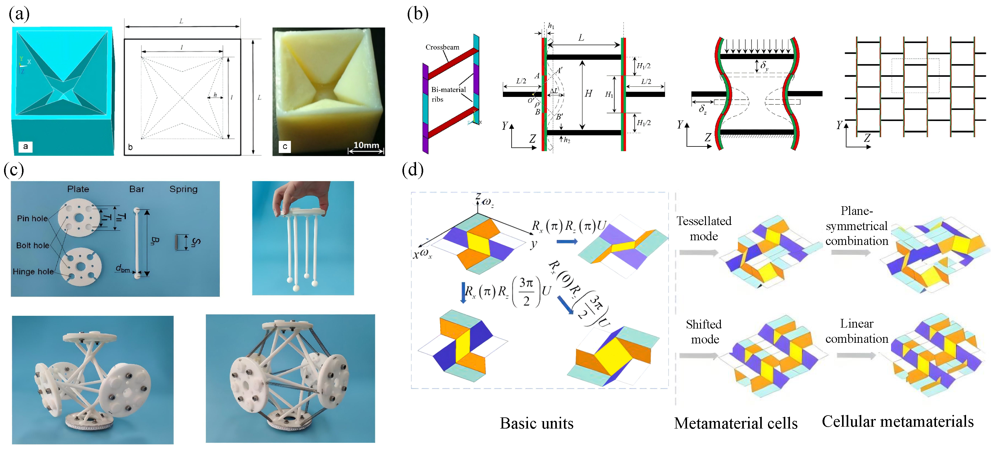
1. Introduction
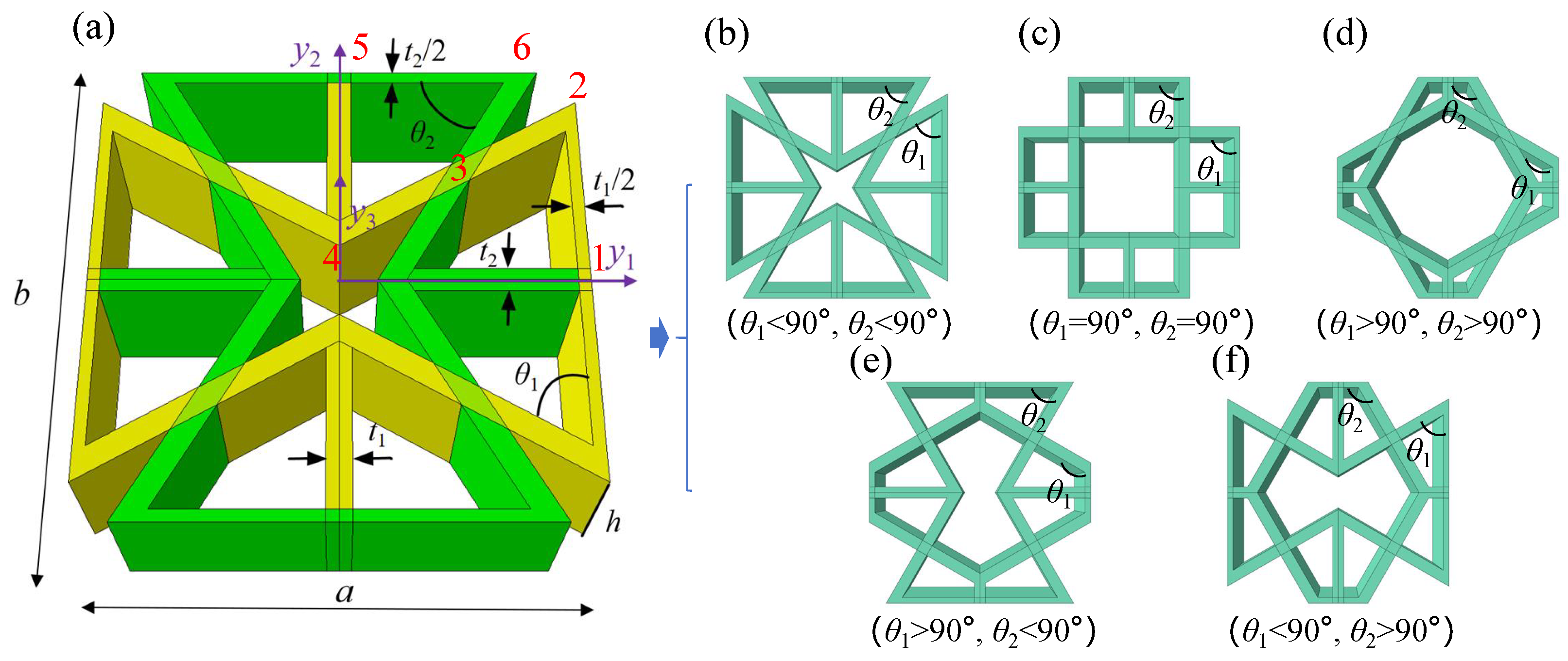
2. Geometry of the Orthogonal Hybrid Honeycomb
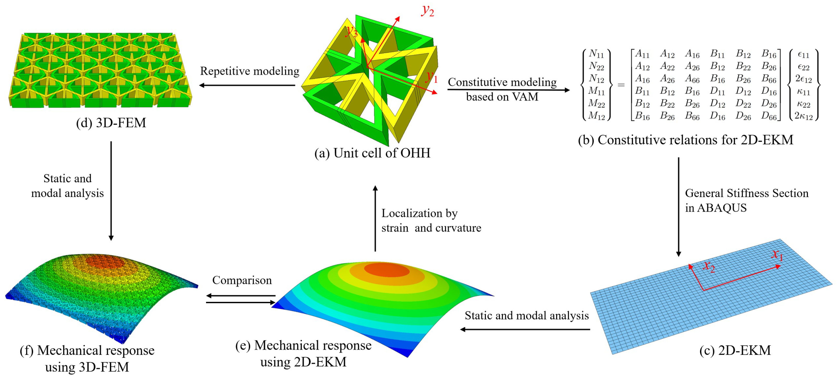
3. VAM-Based Equivalent Plate Model for OHH Panel
3.1. Kinematics of the OHH Panel
3.2. VAM-Based 2D-EKM for the OHH Panel
3.3. Local Field Recovery
4. Model Validation
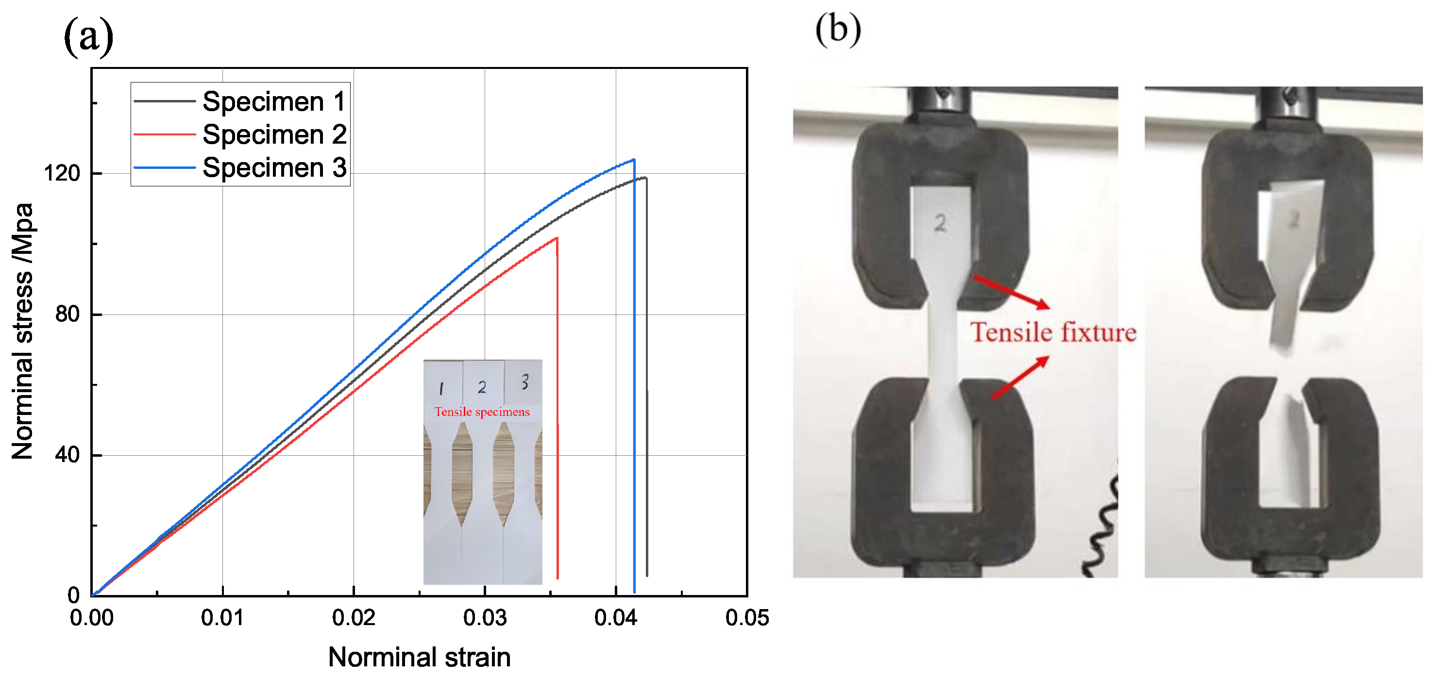
4.1. Experimental Validation
4.1.1. Uniaxial Compression Test
4.1.2. Three-Point Bending Test
4.2. Static and Modal Validation
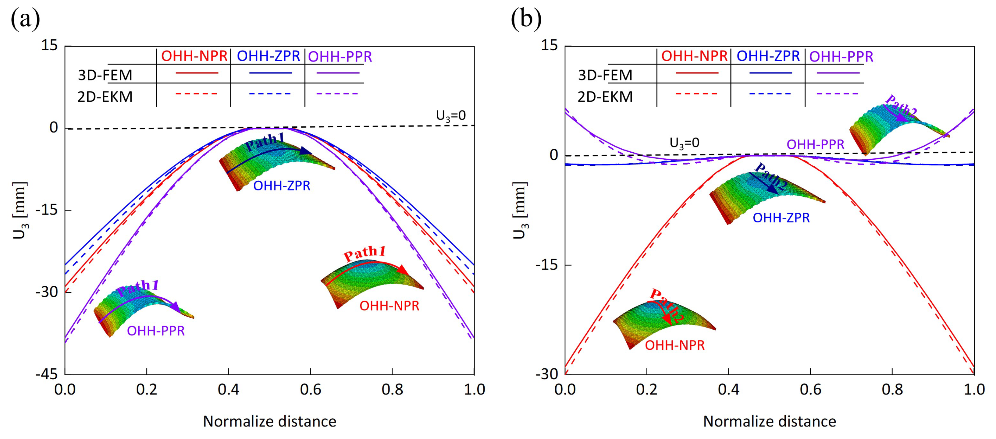
4.2.1. Static Behavior Validation
4.2.2. Local Field Distribution Verification
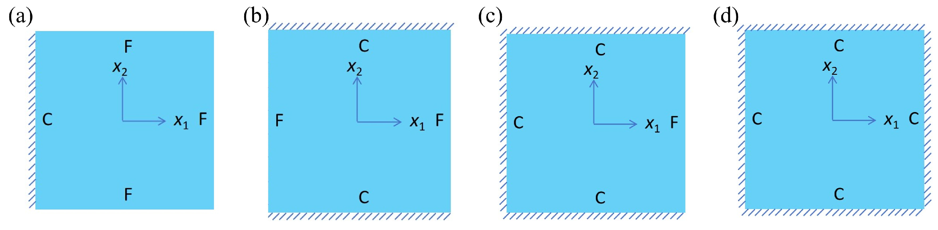
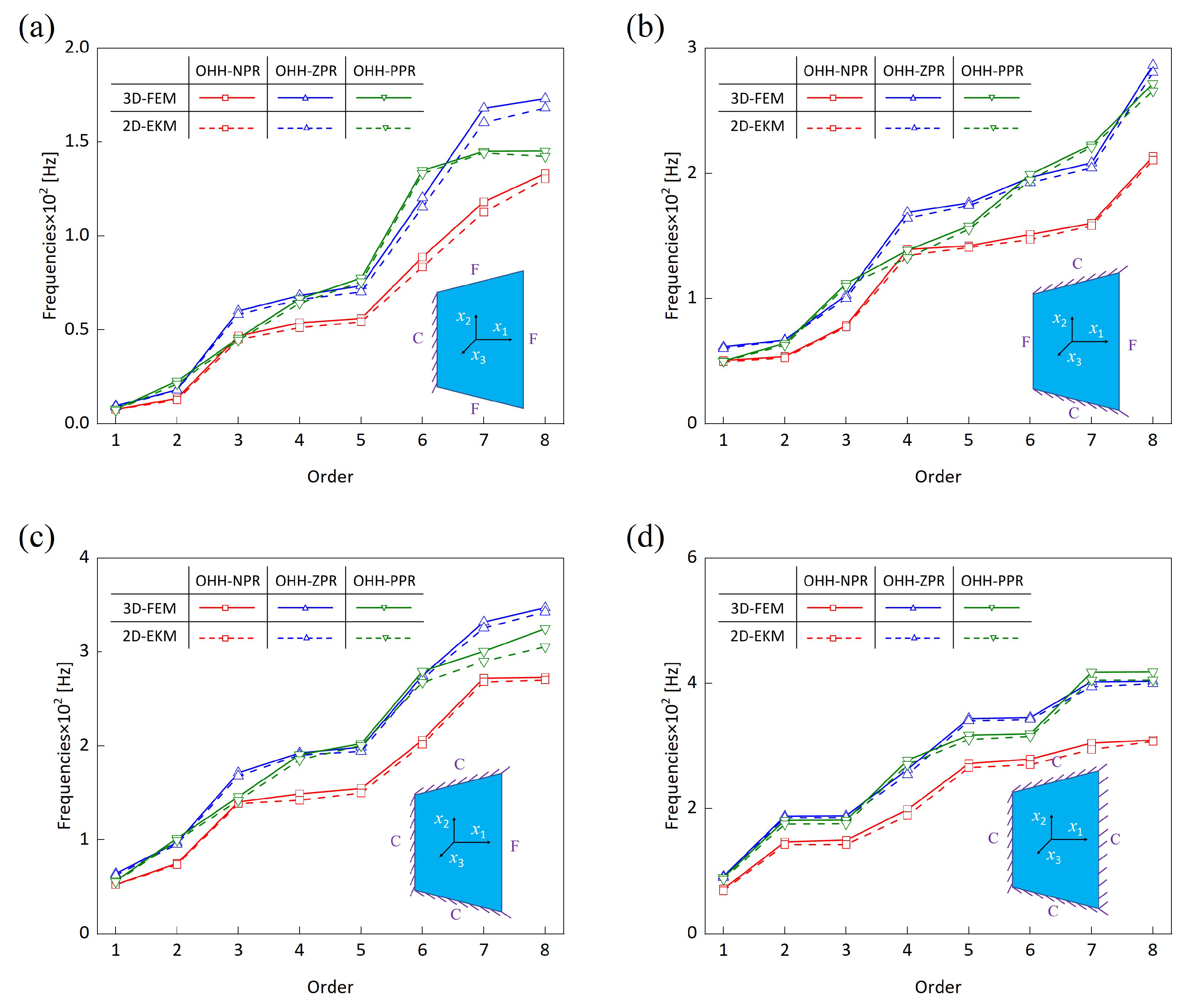
4.2.3. Dynamic Analysis
4.3. Efficiency Comparison
5. Parameter Analysis
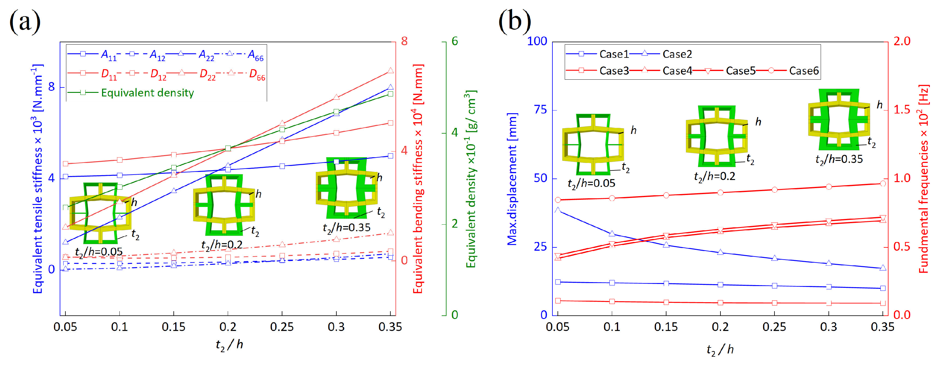
5.1. Wall Thickness–Height Ratio ()
5.2. Wall Thickness–Height Ratio ()
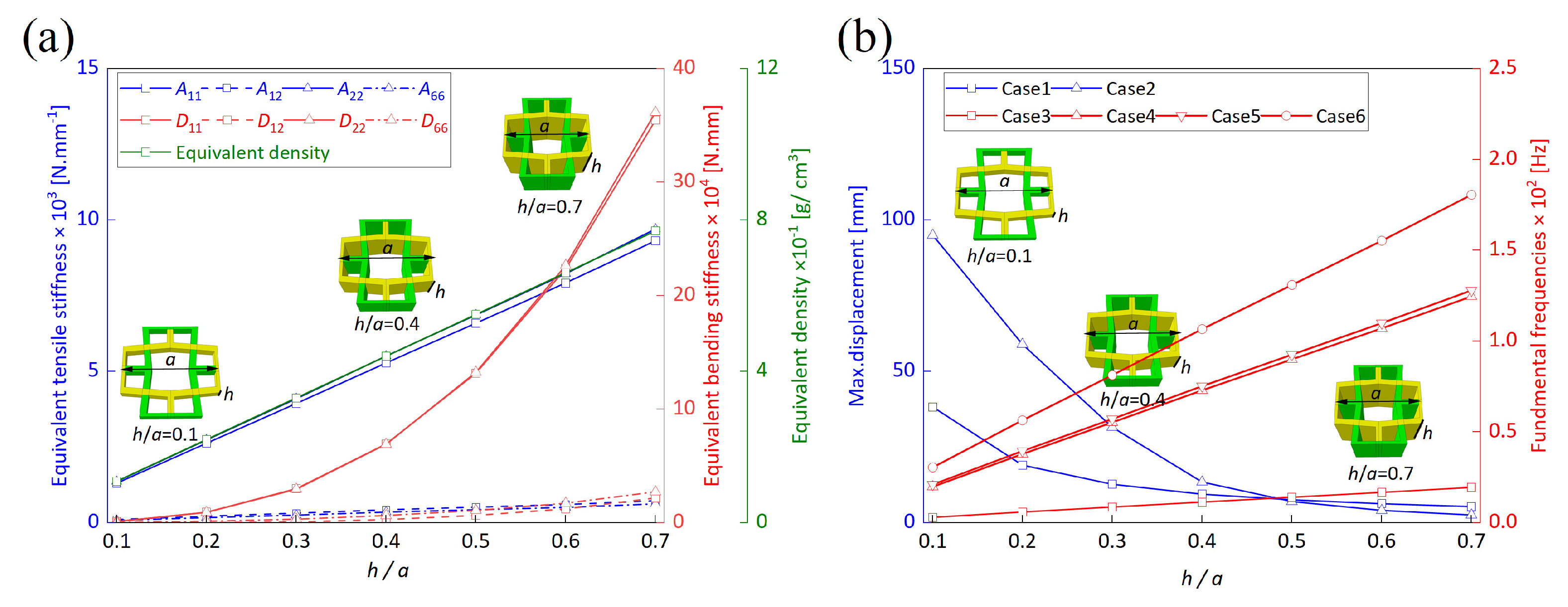
5.3. Height–Length Ratio ()
5.4. Elastic Modulus Ratio of Materials ()
5.5. Summary of Parameter Analysis
6. Conclusions
Author Contributions
Funding
Data Availability Statement
Conflicts of Interest
References
- Chen, Y.; Zheng, B.B.; Fu, M.H. Doubly unusual 3D lattice honeycomb displaying simultaneous negative and zero Poisson’s ratio properties. Smart. Mater. Struct. 2018, 27, 045003. [Google Scholar] [CrossRef]
- Guo, M.F.; Yang, H.; Zhou, Y.M. Mechanical properties of 3D hybrid double arrow-head structure with tunable Poisson’s ratio. Aerosp. Sci. Technol. 2021, 119, 107177. [Google Scholar] [CrossRef]
- Fozdar, D.Y.; Soman, P.; Lee, J.W. Three-dimensional polymer constructs exhibiting a tunable negative Poisson’s ratio. Adv. Funct. Mater. 2011, 21, 2712–2720. [Google Scholar] [CrossRef]
- Lu, H.; Wang, X.; Chen, T. Design and quasi-static responses of a hierarchical negative Poisson’s ratio structure with three plateau stages and three-step deformation. Compos. Struct. 2022, 291, 115591. [Google Scholar] [CrossRef]
- Wang, F. Systematic design of 3D auxetic lattice materials with programmable Poisson’s ratio for finite strains. J. Mech. Phys. Solids. 2018, 114, 303–318. [Google Scholar] [CrossRef]
- Qiao, J.; Chen, C.Q. Analyses on the in-plane impact resistance of auxetic double arrowhead honeycombs. J. Appl. Mech. 2015, 82, 051007. [Google Scholar] [CrossRef]
- Ai, L.; Gao, X.L. Three-dimensional metamaterials with a negative Poisson’s ratio and a non-positive coefficient of thermal expansion. Int. J. Appl. Mech. 2018, 135, 101–113. [Google Scholar] [CrossRef]
- Kelkar, P.U.; Kim, H.S.; Cho, K.H. Cellular auxetic structures for mechanical metamaterials: A review. Sensors 2020, 20, 3132. [Google Scholar] [CrossRef] [PubMed]
- Du Plessis, A.; Razavi, N.; Benedetti, M. Properties and applications of additively manufactured metallic cellular materials: A review. Prog. Mater. Sci. 2022, 125, 100918. [Google Scholar] [CrossRef]
- Scarpa, F. Auxetic materials for bioprostheses. IEEE Signal Process. Mag. 2008, 25, 126–128. [Google Scholar] [CrossRef]
- Zhang, S.L.; Lai, Y.C.; He, X. Auxetic foam-based contact-mode triboelectric nanogenerator with highly sensitive self-powered strain sensing capabilities to monitor human body movement. Adv. Funct. Mater. 2017, 27, 1606695. [Google Scholar] [CrossRef]
- Alderson, A.; Rasburn, J.; Ameer-Beg, S. An auxetic filter: A tuneable filter displaying enhanced size selectivity or defouling properties. Ind. Eng. Chem. Res. 2000, 39, 654–665. [Google Scholar] [CrossRef]
- Grima, J.N.; Jackson, R.; Alderson, A. Do zeolites have negative Poisson’s ratios. Adv. Mater. 2000, 12, 1912–1918. [Google Scholar] [CrossRef]
- Wang, Y.C.; Lakes, R. Analytical parametric analysis of the contact problem of human buttocks and negative Poisson’s ratio foam cushions. Int. J. Solids Struct. 2002, 39, 4825–4838. [Google Scholar] [CrossRef]
- Ma, Y.; Scarpa, F.; Zhang, D. A nonlinear auxetic structural vibration damper with metal rubber particles. Smart Mater. Struct. 2013, 22, 084012. [Google Scholar] [CrossRef]
- Bertoldi, K.; Reis, P.M.; Willshaw, S. Negative Poisson’s ratio behavior induced by an elastic instability. Adv. Mater. 2010, 22, 361–366. [Google Scholar] [CrossRef]
- Cui, S.; Gong, B.; Ding, Q. Mechanical metamaterials foams with tunable negative poisson’s ratio for enhanced energy absorption and damage resistance. Materials 2018, 11, 1869. [Google Scholar] [CrossRef]
- Ai, L.; Gao, X.L. Metamaterials with negative Poisson’s ratio and non-positive thermal expansion. Compos. Struct. 2017, 162, 70–84. [Google Scholar] [CrossRef]
- Greaves, G.N.; Greer, A.L.; Lakes, R.S. Poisson’s ratio and modern materials. Nat. Mater. 2011, 10, 823–837. [Google Scholar] [CrossRef]
- Yu, X.; Zhou, J.; Liang, H. Mechanical metamaterials associated with stiffness, rigidity and compressibility: A brief review. Prog. Mater. Sci. 2018, 94, 114–173. [Google Scholar] [CrossRef]
- Huang, C.; Chen, L. Negative Poisson’s ratio in modern functional materials. Adv. Mater. 2016, 28, 8079–8096. [Google Scholar] [CrossRef] [PubMed]
- Li, D.; Dong, L.; Lakes, R. A unit cell structure with tunable Poisson’s ratio from positive to negative. Mater. Lett. 2016, 164, 456–459. [Google Scholar] [CrossRef]
- Li, D.; Ma, J.; Dong, L.; Lakes, R.S. A bi-material structure with Poisson’s ratio tunable from positive to negative via temperature control. Mater. Lett. 2016, 181, 285–288. [Google Scholar] [CrossRef]
- Yin, X.; Gao, Z.Y.; Zhang, S. Truncated regular octahedral tensegrity-based mechanical metamaterial with tunable and programmable Poisson’s ratio. Int. J. Mech. Sci. 2020, 167, 105285. [Google Scholar] [CrossRef]
- Lyu, S.N.; Qin, B.; Deng, H.C. Origami-based cellular mechanical metamaterials with tunable Poisson’s ratio: Construction and analysis. Int. J. Mech. Sci. 2021, 212, 106791. [Google Scholar] [CrossRef]
- Pagliocca, N.; Uddin, K.Z.; Anni, I.A. Flexible planar metamaterials with tunable Poisson’s ratios. Mater. Des. 2022, 215, 110446. [Google Scholar] [CrossRef]
- Liu, Q.; Zhao, Y. Prediction of natural frequencies of a sandwich panel using thick plate theory. J. Sandw. Struct. Mater. 2001, 3, 289–309. [Google Scholar] [CrossRef]
- Liu, Q.; Zhao, Y. Effect of soft honeycomb core on flexural vibration of sandwich panel using low order and high order shear deformation models. J. Sandw. Struct. Mater. 2007, 9, 95–108. [Google Scholar] [CrossRef]
- Kant, T.; Kommineni, J.R. Large amplitude free vibration analysis of cross-ply composite and sandwich laminates with a refined theory and C finite elements. Comput. Struct. 1994, 50, 123–134. [Google Scholar] [CrossRef]
- Tanimoto, Y.; Nishiwaki, T.; Shiomi, T. A numerical modeling for eigenvibration analysis of honeycomb sandwich panels. Compos. Interfaces 2001, 8, 393–402. [Google Scholar] [CrossRef]
- Wang, Z.; Liu, J. Numerical and theoretical analysis of honeycomb structure filled with circular aluminum tubes subjected to axial compression. Compos. Part B Eng. 2019, 165, 626–635. [Google Scholar] [CrossRef]
- Kumar, A.; Muthu, N.; Narayanan, R.G. Equivalent orthotropic properties of periodic honeycomb structure: Strain-energy approach and homogenization. Compos. Part B Eng. 2023, 19, 137–163. [Google Scholar] [CrossRef]
- Saha, G.C.; Kalamkarov, A.L.; Georgiades, A.V. Effective elastic characteristics of honeycomb sandwich composite shells made of generally orthotropic materials. Compos. Part A Appl. Sci. Manuf. 2007, 38, 1533–1546. [Google Scholar] [CrossRef]
- Sorohan, Ş.; Sandu, M.; Sandu, A.; Constantinescu, D.M. Finite element models used to determine the equivalent in-plane properties of honeycombs. Mater. Today Proc. 2016, 3, 1161–1166. [Google Scholar] [CrossRef]
- Saidi, A.; Coorevits, P.; Guessasma, M. Homogenization of a sandwich structure and validity of the corresponding two-dimensional equivalent model. J. Sandw. Struct. Mater. 2005, 7, 7–30. [Google Scholar] [CrossRef]
- Zhong, Y.F.; Qin, W.; Yu, W. Variational asymptotic homogenization of magnetoelectro-elastic materials with coated fibers. Compos. Struct. 2015, 133, 300–311. [Google Scholar] [CrossRef]
- Cesnik, C.E.; Hodges, D.H. VABS: A new concept for composite rotor blade crosssectional modeling. J. Am. Helicopter Soc. 1997, 42, 27–38. [Google Scholar] [CrossRef]
- Peng, X.; Zhong, Y.F.; Shi, Z. Global buckling analysis of composite honeycomb sandwich plate with negative Poisson’s ratio (CSP-RHC) using variational asymptotic equivalent model. Compos. Stuct. 2021, 264, 113721. [Google Scholar]
- Peng, X.; Zhong, Y.F.; Shi, Z. Free flexural vibration analysis of composite sandwich plate with reentrant honeycomb cores using homogenized plate model. J. Sound Vib. 2022, 529, 116955. [Google Scholar] [CrossRef]
- Miao, S.Q.; Zhong, Y.F.; Zhou, Y.J. Equivalent single-layer model for hierarchical diamond honeycomb sandwich panels using variational asymptotic method. Compos. Struct. 2024, 339, 118149. [Google Scholar]
- Lee, C.Y.; Yu, W.B. Homogenization and dimensional reduction of composite plates with in-plane heterogeneity. Int. J. Solids Struct. 2011, 48, 1474–1484. [Google Scholar] [CrossRef]
- Grima, J.N.; Oliveri, L.; Attard, D. Hexagonal honeycombs with zero Poisson’s ratios and enhanced stiffness. Adv. Eng. Mater. 2010, 12, 855–862. [Google Scholar] [CrossRef]


| Methods | OHH-NPR Cell | OHH-ZPR Cell | OHH-PPR Cell |
|---|---|---|---|
| 3D-EXP | 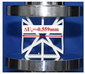 | 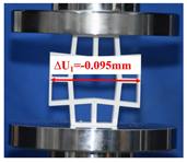 | 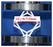 |
| RVE 3D-FEM | 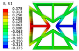 | 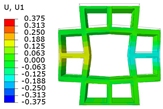 | 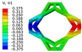 |
| 3D unit cell 2D-EKM | 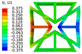 |  |  |
| Models | Legend | OHH-NPR Panel | OHH-ZPR Panel | OHH-PPR Panel |
|---|---|---|---|---|
| 3D-FEM |  |  |  |  |
| 2D-EKM |  |  |  | |
| Error | 8.73% | 6.43% | 4.27% | |
| 3D-FEM |  |  |  |  |
| 2D-EKM |  |  |  | |
| Error | 7.79% | 4.44% | 1.87% | |
| Models | Legend | OHH-NPR Panel | OHH-ZPR Panel | OHH-PPR Panel |
|---|---|---|---|---|
| 3D-FEM |  |  |  |  |
| 2D-EKM |  | 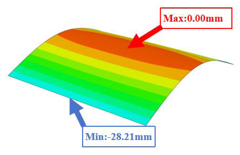 | 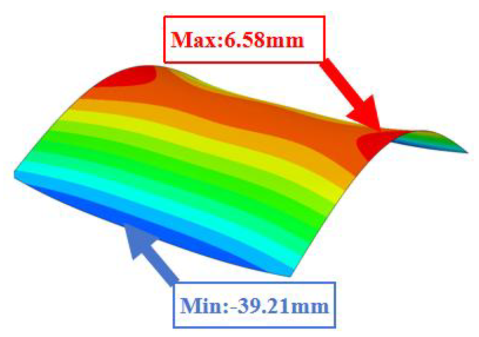 | |
| Error | 8.73% | 6.43% | 4.27% | |
| Cases | Models | Legend | OHH-NPR | OHH-ZPR | OHH-PPR |
|---|---|---|---|---|---|
| Case 1 | 3D-FEM |  |  | 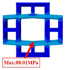 | 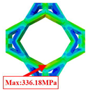 |
| 2D-EKM | 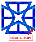 |  |  | ||
| Case 2 | 3D-FEM |  |  |  |  |
| 2D-EKM |  |  |  |
| Models | Case 3 (CFFF) | Case 4 (CCFF) | Case 5 (CCCF) | Case 6 (CCCC) |
|---|---|---|---|---|
| OHH-NPR panel (3D-FEM) |  |  |  |  |
| 7.66 Hz | 50.70 Hz | 52.45 Hz | 71.81 Hz | |
| OHH-NPR panel (2D-EKM) |  | 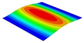 | 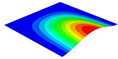 |  |
| 7.59 Hz | 49.58 Hz | 52.24 Hz | 68.96 Hz | |
| OHH-ZPR panel (3D-FEM) |  | 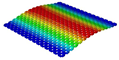 |  |  |
| 9.62 Hz | 61.46 Hz | 64.18 Hz | 91.80 Hz | |
| OHH-ZPR panel (2D-EKM) |  |  | 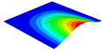 |  |
| 9.05 Hz | 60.12 Hz | 62.34 Hz | 89.82 Hz | |
| OHH-PPR panel (3D-FEM) |  |  |  |  |
| 7.79 Hz | 50.31 Hz | 56.20 Hz | 89.93 Hz | |
| OHH-PPR panel (2D-EKM) |  |  |  |  |
| 7.25 Hz | 50.01 Hz | 55.34 Hz | 87.45 Hz |
| Geometric Parameters | Material Parameter | ||
|---|---|---|---|
| 0.05–0.35 | 0.2 | 0.3 | 1 |
| 0.2 | 0.05–0.35 | 0.3 | 1 |
| 0.3 | 0.3 | 0.1–0.7 | 1 |
| 1 | 1 | 1 | 0.7–1.30 |
Disclaimer/Publisher’s Note: The statements, opinions and data contained in all publications are solely those of the individual author(s) and contributor(s) and not of MDPI and/or the editor(s). MDPI and/or the editor(s) disclaim responsibility for any injury to people or property resulting from any ideas, methods, instructions or products referred to in the content. |
© 2024 by the authors. Licensee MDPI, Basel, Switzerland. This article is an open access article distributed under the terms and conditions of the Creative Commons Attribution (CC BY) license (https://creativecommons.org/licenses/by/4.0/).
Share and Cite
Zhou, Y.; Zhong, Y.; Tang, Y.; Liu, R. Static and Dynamic Characteristics of 3D-Printed Orthogonal Hybrid Honeycomb Panels with Tunable Poisson’s Ratio. Buildings 2024, 14, 2704. https://doi.org/10.3390/buildings14092704
Zhou Y, Zhong Y, Tang Y, Liu R. Static and Dynamic Characteristics of 3D-Printed Orthogonal Hybrid Honeycomb Panels with Tunable Poisson’s Ratio. Buildings. 2024; 14(9):2704. https://doi.org/10.3390/buildings14092704
Chicago/Turabian StyleZhou, Yujie, Yifeng Zhong, Yuxin Tang, and Rong Liu. 2024. "Static and Dynamic Characteristics of 3D-Printed Orthogonal Hybrid Honeycomb Panels with Tunable Poisson’s Ratio" Buildings 14, no. 9: 2704. https://doi.org/10.3390/buildings14092704
APA StyleZhou, Y., Zhong, Y., Tang, Y., & Liu, R. (2024). Static and Dynamic Characteristics of 3D-Printed Orthogonal Hybrid Honeycomb Panels with Tunable Poisson’s Ratio. Buildings, 14(9), 2704. https://doi.org/10.3390/buildings14092704