Abstract
The deformation and damage to seasonal permafrost roadbeds, as seasons shift, stems from the intricate interplay of temperature, moisture, and stress fields. Fundamentally, the frost heave and thaw-induced settlement of soil represent a multi-physics coupling phenomenon, where various physical processes interact and influence each other. In this investigation, a comprehensive co-coupling numerical simulation of both the temperature and moisture fields was successfully executed, utilizing the secondary development module within the finite element software, COMSOL Multiphysics 6.0. This simulation inverted the classical freezing–thawing experiment involving a soil column under constant temperature conditions, yielding simulation results that were in excellent agreement with the experimental outcomes, with an error of no more than 10%. Accordingly, the temperature, ice content, and liquid water content distributions within the seasonal permafrost region were derived. These parameters were then incorporated into the stress field analysis to explore the intricate coupling between the moisture and temperature fields with the displacement field. Subsequently, the frost heave and thaw settlement deformations of the roadbed were calculated, accounting for seasonal variations, thereby gaining insights into their dynamic behavior. The research results show that during the process of freezing and thawing, water migrates from the frozen zone towards the unfrozen zone, with the maximum migration amount reaching 20% of the water content, culminating in its accumulation at the interface separating the two. Following multiple freeze–thaw cycles, this study reveals that the maximum extent of freezing within the roadbed reaches 2.5 m, while the road shoulder experiences a maximum freezing depth of 2 m. A continuous trend of heightened frost heave and thaw settlement deformation of the roadbed is observed in response to temperature fluctuations, leading to the uneven deformation of the road surface. Specifically, the maximum frost heave measured was 51 mm, while the maximum thaw settlement amounted to 13 mm.
1. Introduction
In recent years, the exponential expansion of rail transit engineering has posed novel challenges to construction endeavors in extreme cold regions, notably in highway construction [1,2]. Permafrost, a unique geological blend of soil and ice, exhibits intricate instabilities, governed by intricate interactions between water, heat, and mechanical forces. Consequently, roadbeds constructed in permafrost regions are susceptible to two primary types of detrimental effects: frost heaving, which results from water expansion upon freezing, and thaw settlement, occurring as the ice melts and the ground subsides [3,4]. It is evident that the physical and mechanical properties of seasonal permafrost roadbeds are predominantly influenced by temperature fluctuations and water content, both of which play pivotal roles in determining their stability and durability [5].
Under fluctuating temperatures, roadbeds within seasonal permafrost zones experience cycles of freezing and thawing, where soil freezing is triggered by the migration of water under temperature gradients. This migration process is intricately intertwined with the phase change between ice and water, where the heat liberated during this transformation decelerates the rate of water migration. Furthermore, the formation of ice acts as a barrier, impeding the movement of unfrozen water. Consequently, the intricate water–heat coupling mechanisms within permafrost represent a critical area of research focus [6,7]. Through field observations and experiments, Tabe established that water migration is the primary driver of frost heaving, introducing the capillary theory [8]. Everett further elaborated on the thermodynamics behind the formation of “ice lenses” in porous materials, considering the damage to roads and buildings caused by freezing, refining the capillary theory [9]. While this theory offers a clear understanding of ice formation mechanisms, its quantitative application remains challenging. In response, Harlan drew parallels between fluid transfer in partially frozen soil and, in unsaturated soil, disregarded ice lens formation to model the effects of temperature and water content on fluid movement [10]. Taylor and Luthin then introduced the concept of “ice impedance”, positing that ice hinders water migration in permafrost, thereby simplifying Harlan’s model [11].
In recent years, numerous academics have advanced water–heat coupling models that encompass comprehensive frameworks for water–heat migration equations, ice–water phase transitions, and intricate soil deformation calculations. Zhan et al. constructed a water–heat–stress coupling model to investigate the frost heave deformation characteristics of soil slopes in seasonal areas [12]. Booshehrian et al. defined the relationship between unfrozen water content and cryogenic suction, based on the similarity between soil freezing and soil–water characteristic curves for unsaturated soils [13]. Mihara et al. modified the Soil and Water Assessment Tool (SWAT), by incorporating the dynamic change in soil permeability based on the degree of soil freezing [14]. Yin et al. established a mathematical model for the coupling of liquid, vapor, and heat fields [15]. Li et al. established a finite element model, which considered the effect of thermo–hydro–mechanical coupling, to investigate the freezing damage of berms under the influence of the reservoir level and the water migration of dam filling [16]. Lu et al. proposed different modeling approaches by regarding the environmental factor as a constitutive variable and introducing the 3D fractional plastic flow rule into the characteristic stress space [17,18]. Zhang et al. carried out an extensive series of pore water pressure tests under sub-zero conditions, delving into the dynamics of how pore water pressure fluctuates and subsequently influences deformation patterns [19].
Despite the fact that extensive theoretical and experimental investigations have been conducted on permafrost deformation, which have mainly focused on the final results of stable deformation and the main influencing factors, there are limitations to the modeling of moisture transport in permafrost. Scarce attention has been paid to the implications of coupled water–heat variations on the stability of roadbed deformation and, consequently, there exists a notable dearth of models that have been effectively applied to practical engineering contexts.
Hence, this study is based on the construction of the Shuang-Tao expressway roadbed. The theoretical and numerical simulation methods are combined to study the water–heat coupling process and the deformation of the roadbed. First, the coupling model was simplified by incorporating a solid–liquid ratio and relative saturation, considering the influence of ice–water phase transitions on the water–heat distribution. This refined model is then implemented within the COMSOL software framework, to replicate and analyze classic freezing and thawing experiments on soil columns. Through secondary development, the rationality and accuracy of the established model were validated. Subsequently, the validated coupling model was applied to the Shuang-Tao expressway roadbed, leveraging numerical simulations to comprehensively characterize the roadbed’s water, heat, and stress states, as well as their dynamic variations over time. Finally, the intricate patterns and trends governing the evolution of the roadbed’s water content field, temperature field, and deformation field were investigated, thereby providing valuable insights into the roadbed’s performance and durability.
2. The Water–Heat Coupling Model
Seasonal permafrost undergoes cyclic variations driven by external temperature fluctuations, leading to seasonal cycles of freezing and thawing. These processes can induce detrimental effects on roadbeds, including cracking, frost heave, and thaw-induced settlement. The primary underlying mechanism is the migration and phase transformation of water within the roadbed soil, during these temperature-driven transitions. Hence, the present study delves into the alterations in temperature and moisture distributions within roadbeds during freeze–thaw cycles. Leveraging a water–heat coupling mathematical framework, this research employs the COMSOL finite element software to perform comprehensive, coupled simulations of both temperature and moisture fields, achieved through tailored secondary development.
This study assumes the following premises: (1) the roadbed soil is modeled as a homogeneous, isotropic, and porous elastic medium; (2) water migration between frozen and unfrozen zones in the roadbed occurs exclusively in the liquid phase; (3) the soil particles, ice, and water are considered incompressible; (4) the movement of liquid water within the roadbed adheres to Darcy’s law; and (5) heat variations in the roadbed soil are primarily attributed to heat conduction and the phase transformations of ice and water, while other modes of heat transfer are deemed negligible.
2.1. Water–Heat Coupling Differential Equations
Due to the elongated nature of the roadbed along the longitudinal axis and its significantly reduced dimensions in perpendicular directions, the analysis of its moisture field can be simplified and focused on the cross-sectional plane, thereby transforming the study into a two-dimensional problem of academic rigor. Based on Darcy’s law [20] and the principle of mass conservation [21], the governing equation for the migration of permafrost moisture can be obtained as:
The seasonal fluctuations in moisture within permafrost roadbeds elicit phase transformations, resulting in non-steady-state thermal variations. To tackle this phase change challenge utilizing the specific heat capacity approach, it is assumed that there are no extraneous heat sources within the soil. Drawing upon heat conduction theory, a two-dimensional, non-steady-state temperature field heat conduction differential equation is obtained as Equation (2), which is tailored specifically for roadbeds undergoing phase transformations [22].
Equations (1) and (2) reveal three unknowns, namely the liquid water content, ice content, and temperature, yet only two fundamental equations are provided. To ensure a comprehensive and solvable water–heat coupling system, a third, supplementary relationship is essential. This research introduces the concept of the “solid–liquid ratio”, B1, which quantifies the proportion of solid ice to liquid water within the permafrost, thereby completing the mathematical framework.
2.2. Water–Heat Coupling Numerical Model
Based on the aforementioned model, this study utilized the secondary development of the PDE module within the COMSOL software to achieve the coupling of the moisture and temperature field. The pertinent equations and boundary constraints are outlined as follows:
By converting Equations (1) and (2) into the coefficient form of the partial differential equation group provided by COMSOL, the coupling solution can be achieved.
- (1)
- Modeling of the water field
Firstly, the partial differential Equation (4) is written in a customized form as:
Next, Equation (1) is transformed into the form of a coefficient-type partial differential equation, as follows:
Based on the VG hysteresis model and the Gardner permeability coefficient model [23], the saturation degree S of the permafrost can be defined as:
Substituting Equations (3) and (9) into Equation (8) yields:
Subsequently, the coefficients of the partial differential equation can be obtained as:
where e, α, and β are all set to 0.
- (2)
- Modeling of the temperature field
First, the partial differential Equation (4) is rewritten as follows:
Subsequently, Equation (2) is expressed in the form of a coefficient-type partial differential equation, as follows:
Based on the principle of establishing the moisture field model, the following can be derived as:
Consequently, the coefficients of the partial differential equation are obtained as follows:
where e, α, λ, a, and β are all set to 0.
2.3. Validation of Numerical Model
To validate the efficacy and practical applicability of the aforementioned heat–moisture coupled model, the model was used to invert an enclosed columnar soil freezing and thawing experiment, as conducted by Xu et al. [24].
2.3.1. Freezing Simulation Validation and Analysis
The test soil sample was composed of silty soil, with a diameter (d) of 10 cm and a height (h) of 15 cm. The initial moisture content was 18.6%. The top plate temperature was maintained at 0.9 °C, while the bottom plate temperature was set to −2.1 °C. The initial temperature was kept constant at 0.9 °C. The lateral sides of the soil column were insulated and impermeable, and there was no water supply at the bottom boundary. The values of the soil parameters required for the model calculations are listed in Table 1.

Table 1.
Table of calculation parameters of soil column.
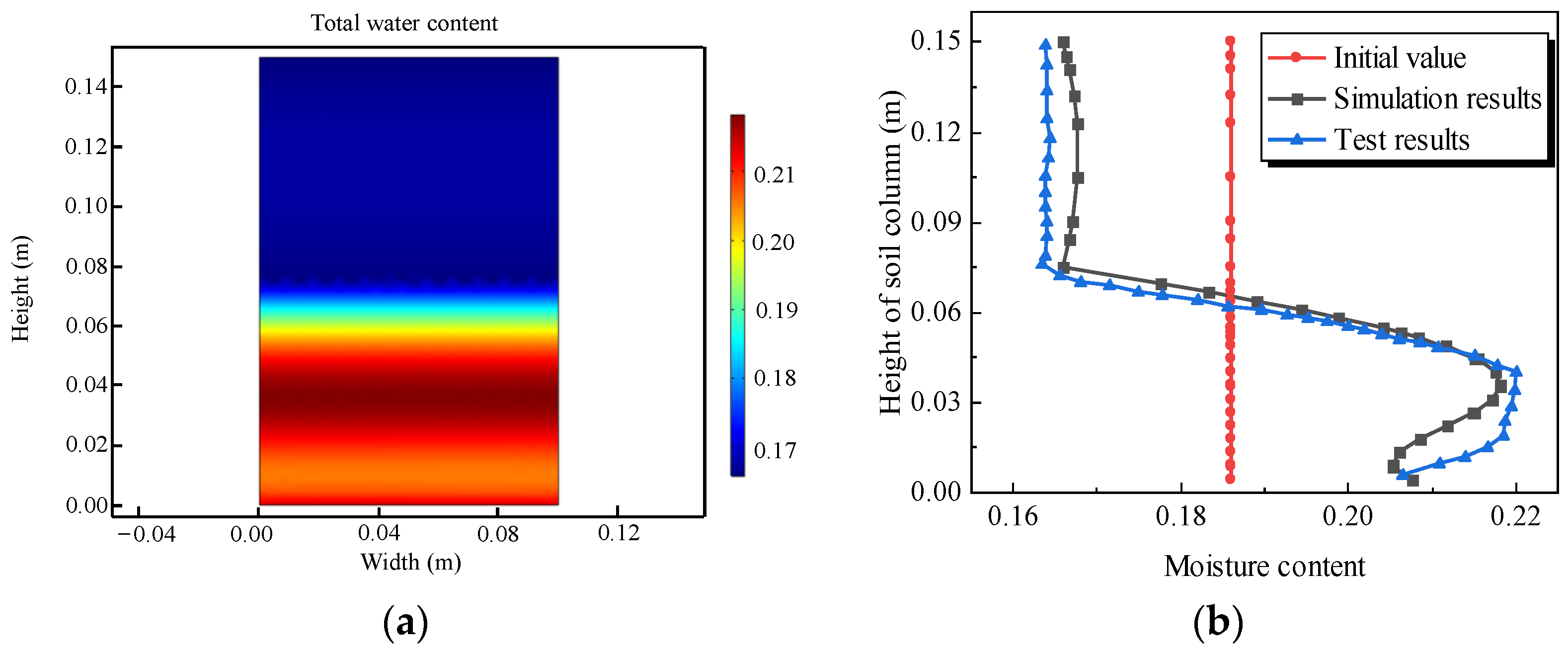
The numerical simulation results of the freezing test were compared with the corresponding test results, as presented in Figure 1. Freezing was initiated from the bottom and resulted in a significant increase in the moisture content in the lower portion compared to the pre-freezing state, while the upper portion exhibited a noticeable decrease. This indicated that water migrated from the top to the bottom during the freezing process. The liquid water content in the freezing zone decreased, leading to an increase in suction. Under the capillary action, moisture from the thawing zone in the upper part of the soil column migrated towards the freezing front. Some of it froze near the freezing–thawing interface, while the rest was impeded by the ice, resulting in an increase in the moisture content in the freezing zone, with the appearance of a peak value. When the temperature field approached stability, the final height of the freezing–thawing interface was approximately 7.5 cm and the simulated temperature at the interface was approximately −0.57 °C. Moreover, compared to the temperature field, the moisture field exhibited hysteresis, with moisture migration not immediately reaching equilibrium once the temperature became stable. Instead, it continued to migrate for a certain period of time, ultimately leading to the appearance of a moisture content peak below the freezing–thawing interface. In addition, it can be seen from Figure 1b that the vertical distribution of the moisture content obtained from the numerical simulation was in good agreement with the test results; the average relative error was 1.5%, indicating the numerical simulation accurately reflected the variation characteristics of the water field during the freezing process of frozen soil.
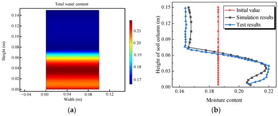
Figure 1.
Variation in freezing water content: (a) cloud map and (b) vertical distribution.
2.3.2. Thawing Simulation Validation and Analysis
The simulation of the thawing test was modeled in reference to the freezing test, with consistent soil and model parameters. However, unlike the freezing test, the initial temperature was kept constant at −2.1 °C, and the water content distribution after 120 h is presented in Figure 2. During the soil column thawing process, the height of the frozen–thawed zone interface and the simulated freezing temperature value were consistent with the freezing test, respectively, 7.5 cm and −0.57 °C. The liquid water content above the frozen–thawed zone interface decreased gradually and uniformly, while the liquid water content below the frozen–thawed zone interface increased vertically from bottom to top. The water content at the frozen–thawed zone interface increased with time and, after the frozen–thawed zone interface stabilized, an increasing trend in the water content could be observed. The variation trend in the total water field in the soil column was basically consistent with the final result of the laboratory thawing test, with an average relative error of 8.5%, verifying the rationality of the water–heat coupling model.
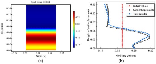
Figure 2.
Variation in liquid water content: (a) cloud map and (b) vertical distribution.
3. Deformation Analysis of Seasonal Frozen Roadbed
The aforementioned numerical simulation of water–heat coupling was applied to investigate the temperature and water fields in the permafrost roadbed of the Shuang-Tao expressway. Firstly, the fully coupled calculation of the water and heat fields of the roadbed was conducted to obtain the distribution of the temperature, ice content, and liquid water content. Then, the data was imported into the stress field to analyze the coupling of the water and temperature fields with the displacement field, and to calculate the deformation and stress of the roadbed, achieving the seasonal permafrost full water–heat coupling and deformation analysis of the roadbed.
3.1. Project Overview
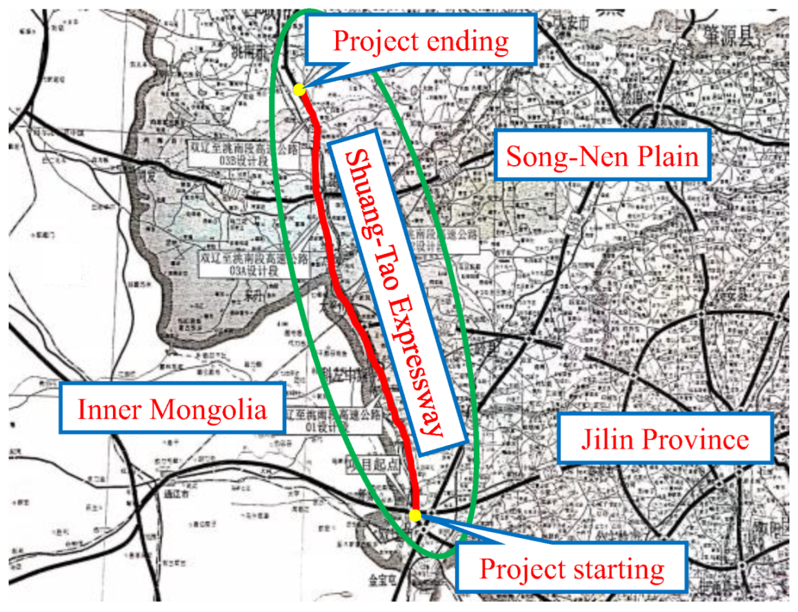
The Shuang-Tao expressway is located in the western region of Jilin province, China, as shown in Figure 3. It is an important longitudinal, regional distribution expressway. The expressway belongs to the mid-temperature zone of the continental monsoon climate, with significant seasonal changes. Spring is dry and windy, summer is hot and rainy, autumn is cool with large temperature differences between day and night, and winter is long and cold.
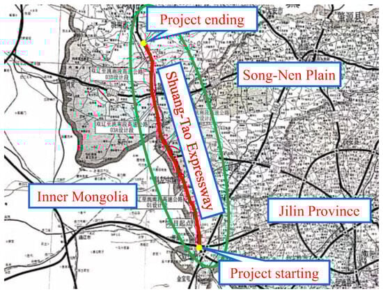
Figure 3.
Shuang-Tao expressway project line.
3.2. Water–Heat Coupling Analysis
3.2.1. Parameters of the Model
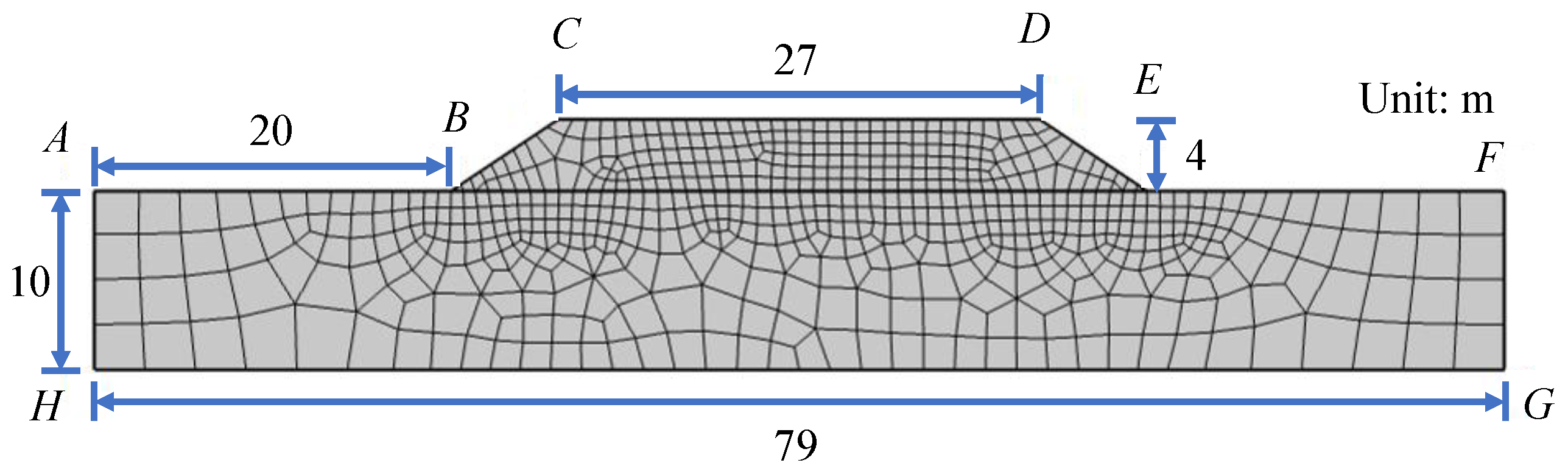
The width of the roadbed was 27 m, the height was 4 m, and the side slope was 1:1.5. The depth below the roadbed was 10 m. When the boundaries of the model were far enough, the effect of the temperature field of the roadbed on the original seasonal permafrost could be ignored [25]. Therefore, the outward length on each side was taken as 20 m. The roadbed fill was gravel soil and the foundation was powdery clay. The model adopted a free quadrilateral mesh and the roadway section was densified, as shown in Figure 4. The selected parameters for the roadbed are shown in Table 2 and Table 3.
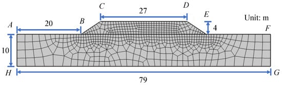
Figure 4.
Geometric model and meshing of the roadbed.
Table 2.
Thermodynamic parameters.
Table 3.
Hydraulic parameters.
3.2.2. Boundary Conditions and Simulation Process
- (1)
- Temperature boundary conditions
Considering the actual situation, the surface temperature of the roadbed was described by the following equation based on the local temperature:
where T is the surface temperature of the roadbed (°C), T0 is the average annual temperature (°C), A is the annual amplitude of the fluctuation in the daily average temperature (°C), t is time (d), and φ0 is the first phase.
Based on the temperature in Jilin province, the annual average temperature was taken as 7.4 °C and the annual maximum temperature difference was 52 °C. Taking 18 October 2019, as the starting point for the temperature, φ0 was taken as π and a vertical temperature gradient was not considered. Hence, the temperature boundary condition of the upper boundary of the roadbed model was as follows:
Assuming that the left and right boundaries, AH and FG, respectively, were sufficiently distant, they could be regarded as adiabatic, thereby neglecting any heat exchange across these interfaces. The deeply embedded bottom boundary GH experienced minimal temperature fluctuations due to the external environment, maintaining a nearly constant temperature of 9 °C. The soil’s freezing point Tf was set at −0.4 °C.
- (2)
- Moisture boundary conditions
Within the numerical model, the roadbed was considered a closed system, neglecting precipitation and evaporation impacts on moisture. Based on engineering specifications, the initial soil moisture content was set at 12.36%.
- (3)
- Initial conditions
To minimize computational errors, the thermal boundary conditions on the roadbed’s top surface were initially derived using Equation (17). Subsequently, the roadbed’s temperature field was simulated over 50a, and the stabilized temperature distribution was adopted as the initial condition for subsequent temperature analysis.
3.2.3. Results and Discussion
- (1)
- Temperature field
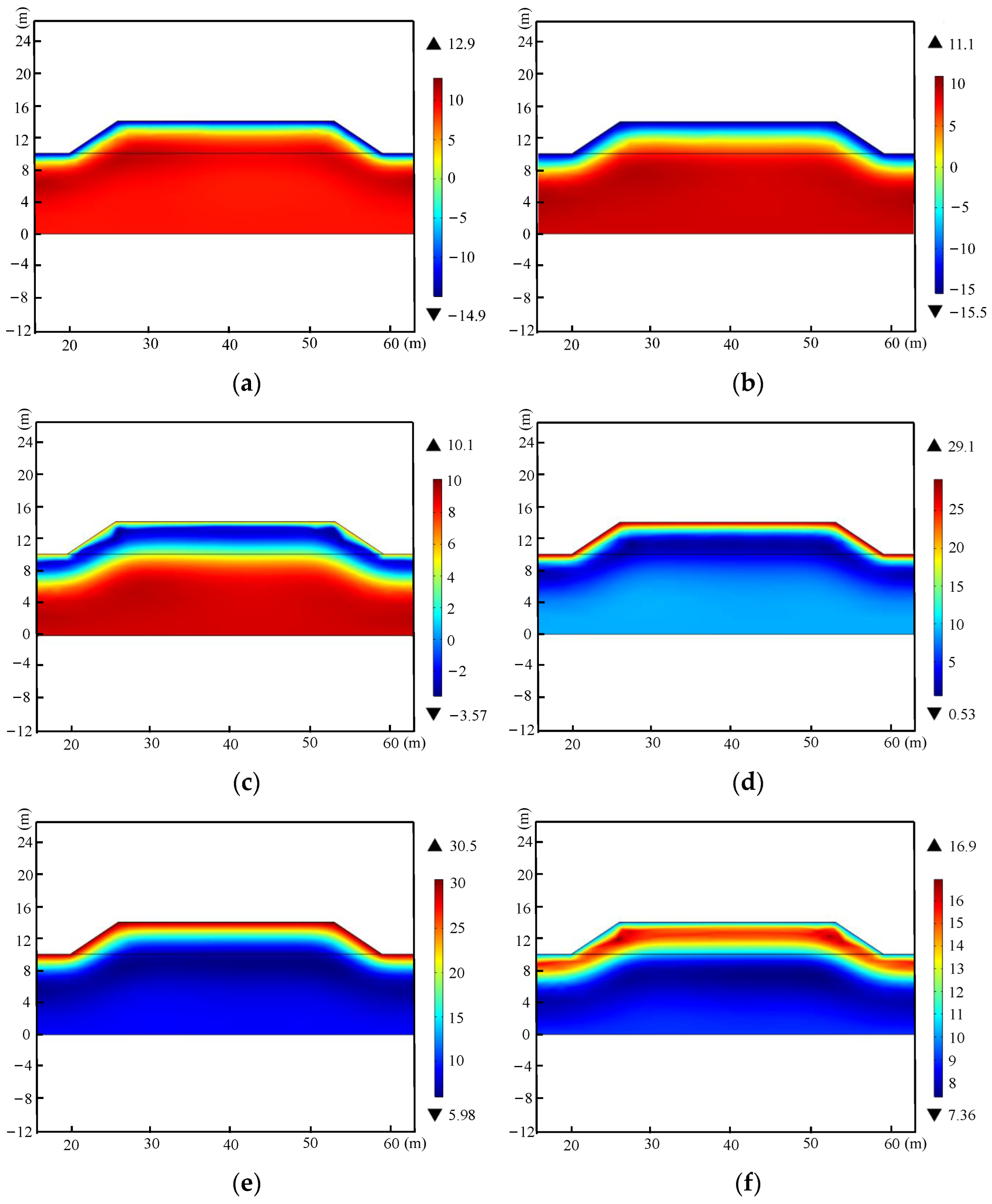
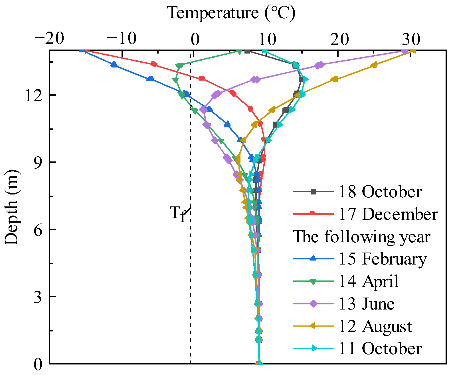
To investigate seasonal variations in the ground temperature within a permafrost roadbed, a water–heat coupling analysis was conducted, with subsequent analysis of the roadbed temperature distributions every 60 days, commencing from 18 October of the initial year. As presented in Figure 5 and Figure 6, with a decrease in the external temperature, the temperature of the upper boundary of the roadbed dropped to −15 °C on 17 December, reaching the soil’s freezing point, resulting in a 1.3 m deep frozen layer within the roadbed. By 15 February of the subsequent year, the upper boundary temperature stabilized at −15 °C, with the frozen depth extending to approximately 2 m, due to the extended freezing duration. Below this depth, temperatures remained above the freezing point, gradually approaching the initial temperature. On 14 April of the same year, with ambient temperatures rising to 7 °C, the roadbed temperature commenced an upward trend. Nevertheless, pockets of sub-zero soil persisted within the roadbed. Heat transfer occurred bidirectionally, with warmth ascending from deep layers and descending from the surface, initiating a thawing process marked by heat absorption. Despite an overall temperature increase, the frozen depth paradoxically expanded from 2 to 2.5 m. On 13 June, with sustained temperature increases, all soil layers within the roadbed surpassed the freezing point, with the temperature nadir observed at a depth of approximately 2.5 m. On 12 August, the roadbed’s temperature hovered around 30 °C, with the soil’s coolest point located at a depth of approximately 5 m. This phenomenon stems from bidirectional heat transfer, with both shallow and deep, warmer zones simultaneously transferring heat to cooler regions. Consequently, the depth of the lowest temperature shifted from 2.5 to 5 m. In October of the subsequent year, with ambient temperatures declining to approximately 7 °C, the roadbed’s temperature distribution mirrored that observed in October of the initial year. Upon crossing the freezing threshold, a fresh freeze–thaw cycle was initiated.
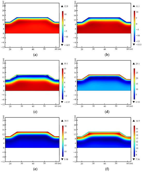
Figure 5.
Temperature variation in the roadbed in one year: (a) 17 December, (b) 15 February, (c) 14 April, (d) 13 June, (e) 12 August, and (f) 11 October.
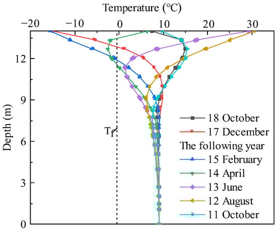
Figure 6.
Variation in the temperature in terms of the depth at the center of the roadbed, in one year.
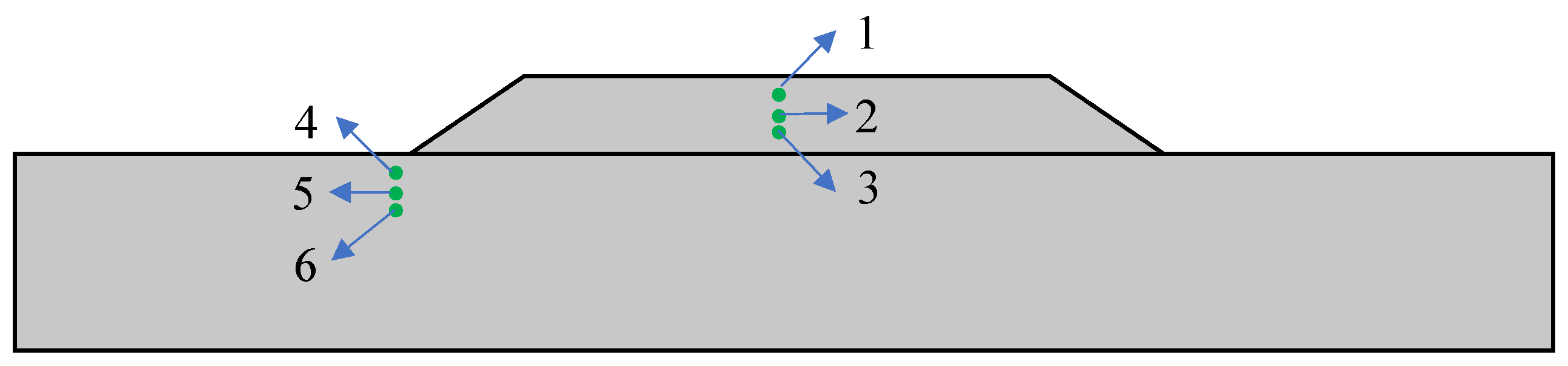
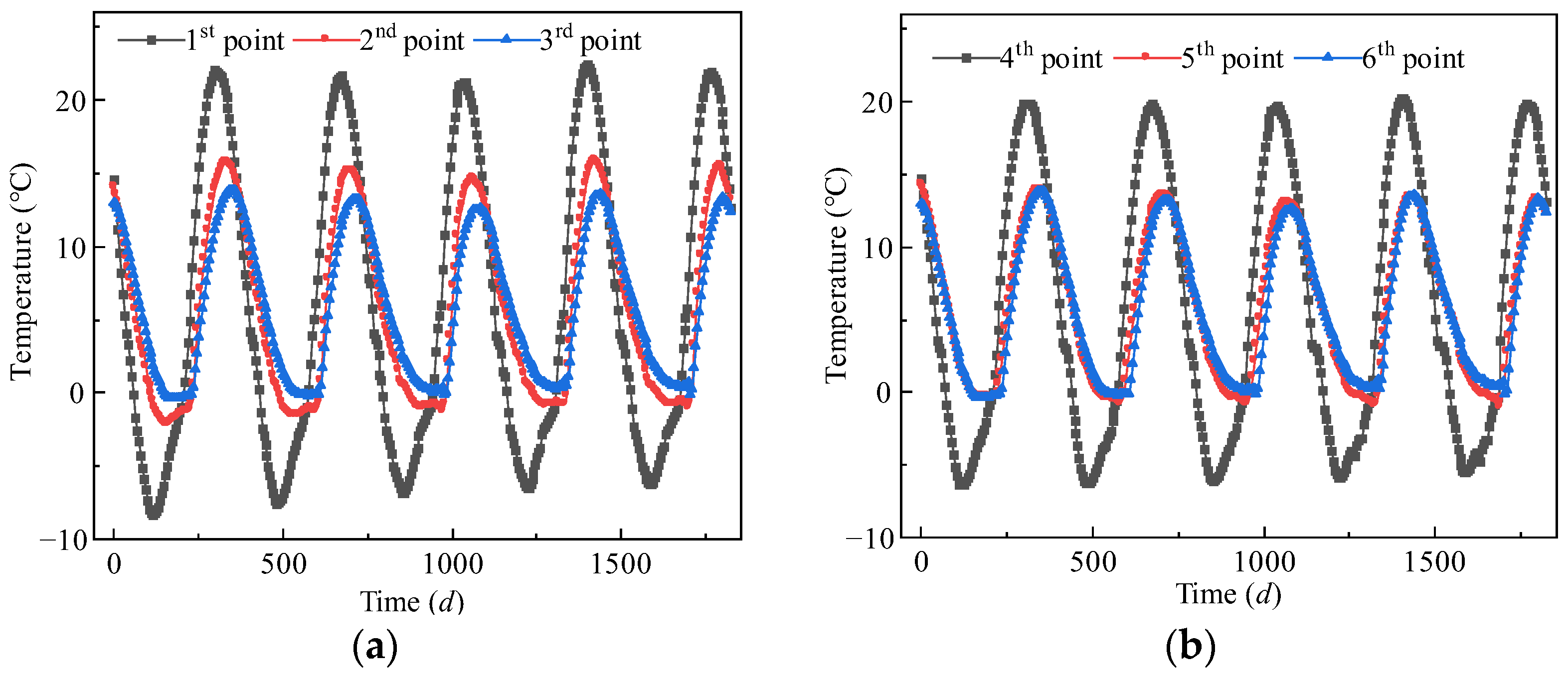
As depicted in Figure 7, the first, second, and third control points were positioned at depths of 1, 2, and 2.5 m, respectively, below the roadbed’s centerline. Meanwhile, the fourth, fifth, and sixth control points were situated at depths of 1, 2, and 2.5, respectively, beneath the natural ground surface, 0.5 m lateral to the left slope foot. Figure 8 illustrates the temporal temperature variation curves for the six control points, revealing a sinusoidal trend that aligns with fluctuations in the boundary temperatures. A consistent pattern of temperature variation was evident across all six points. However, the soil’s inherent temperature lag response accounts for the delayed increase in temperatures at points 2 and 3 beneath the roadbed, even as point 1 initiates an upward trend. This lag necessitates varying durations for each depth’s controlled point to attain maximum or minimum temperatures. During the freezing period, the roadbed soil at equivalent depths exhibited temperatures 1 °C to 2 °C higher than the foundation soil. Similarly, during soil warming, the roadbed soil retained higher temperatures, attributable to its more pronounced temperature variations compared to the foundation soil. Control points 5 and 6 recorded a minimum temperature of approximately 0 °C, confirming a foundation freezing depth of ~2 m, aligned with the observed conditions. Point 2’s minimum temperature was also ~0 °C, whereas point 3 dipped below freezing, indicating a roadbed freezing depth of ~2.5 m. This establishes the order of the depth-based influence of the ground temperature as roadbed > natural ground surface.

Figure 7.
Position of control points in the roadbed.
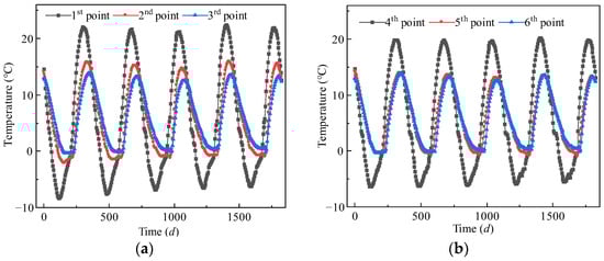
Figure 8.
Change in control point temperature in 5 years: (a) below the roadbed surface and (b) below the natural ground surface.
- (2)
- Moisture field
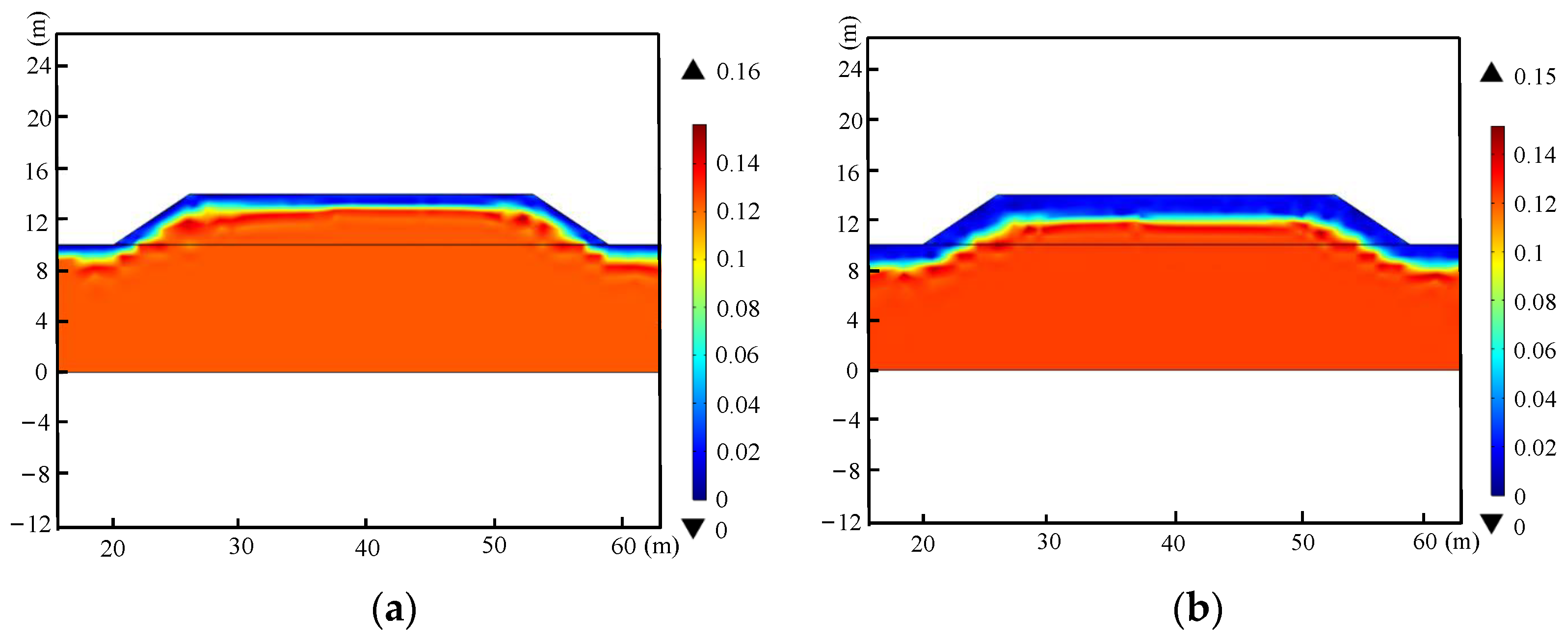
Based on the time points of the temperature field, the annual variations in liquid water and ice content within the seasonal permafrost roadbed, correlated with the external temperature fluctuations, as depicted in Figure 9, Figure 10 and Figure 11. On 17 December, the roadbed’s upper boundary temperature fell below freezing point, resulting in a 1.3 m deep frozen zone. The ice content within this zone correlated positively with the decreasing temperatures, peaking at 23%, while the liquid water content remained low at 2%. The ice barrier promoted liquid water migration towards the freeze–thaw interface, causing an increase in the liquid water content (max 13%) within the 1.3–2 m zone. On 15 February of the subsequent year, the upper boundary temperature remained low, leading to a downward progression in the freezing front and an expansion of the frozen zone to a 2.5 m depth. Concurrently, a slight increase in the liquid water content was observed proximate to the newly formed freezing surface. By 14 April of this year, the ambient temperature surpassed freezing, initiating thawing in the shallow frozen zone and an increase in the liquid water content. Despite this, pockets of sub-zero temperatures persisted in the roadbed, prompting liquid water migration from both the superficial and deeper layers towards the residual freezing zone, resulting in enhanced liquid water content approximately 1 m deep within this zone. After 13 June, the roadbed underwent complete thawing due to temperature elevation, minimizing water migration. Until the next freeze–thaw cycle, the roadbed’s liquid water content distribution remained stable. Water migration led to an increase in the surface water content, from 12.3% to 22%.
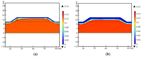
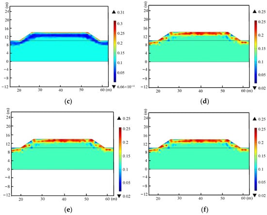
Figure 9.
Variation in the liquid water content of the roadbed in one year: (a) 17 December, (b) 15 February, (c) 14 April, (d) 13 June, (e) 12 August, and (f) 11 October.

Figure 10.
Variation in the ice content of the roadbed in one year: (a) 17 December, (b) 15 February, (c) 14 April, and (d) 13 June.
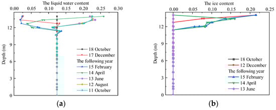
Figure 11.
Variations in the liquid water and ice content in the center of the roadbed according to different depths in one year: (a) the liquid water content and (b) the ice content.
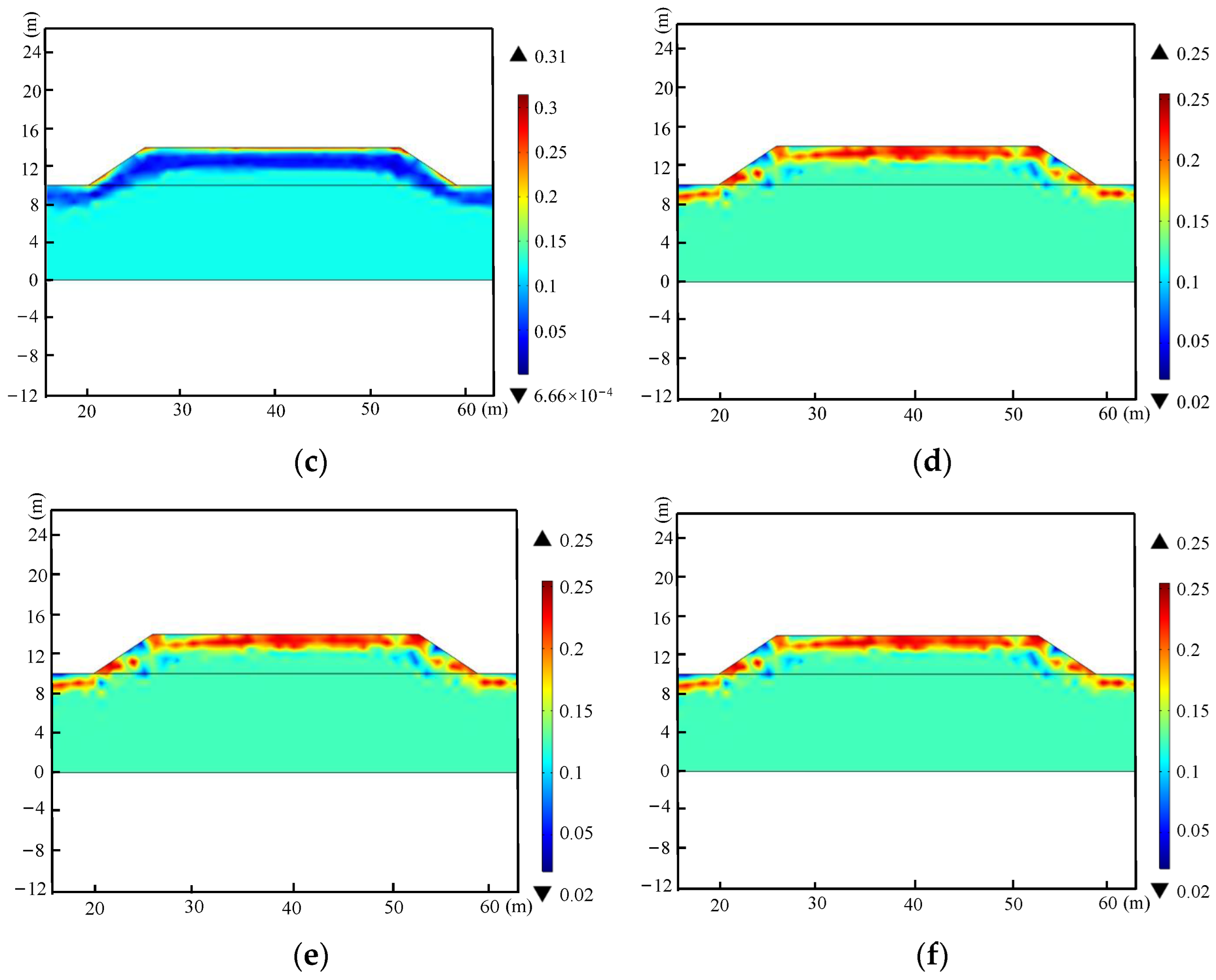
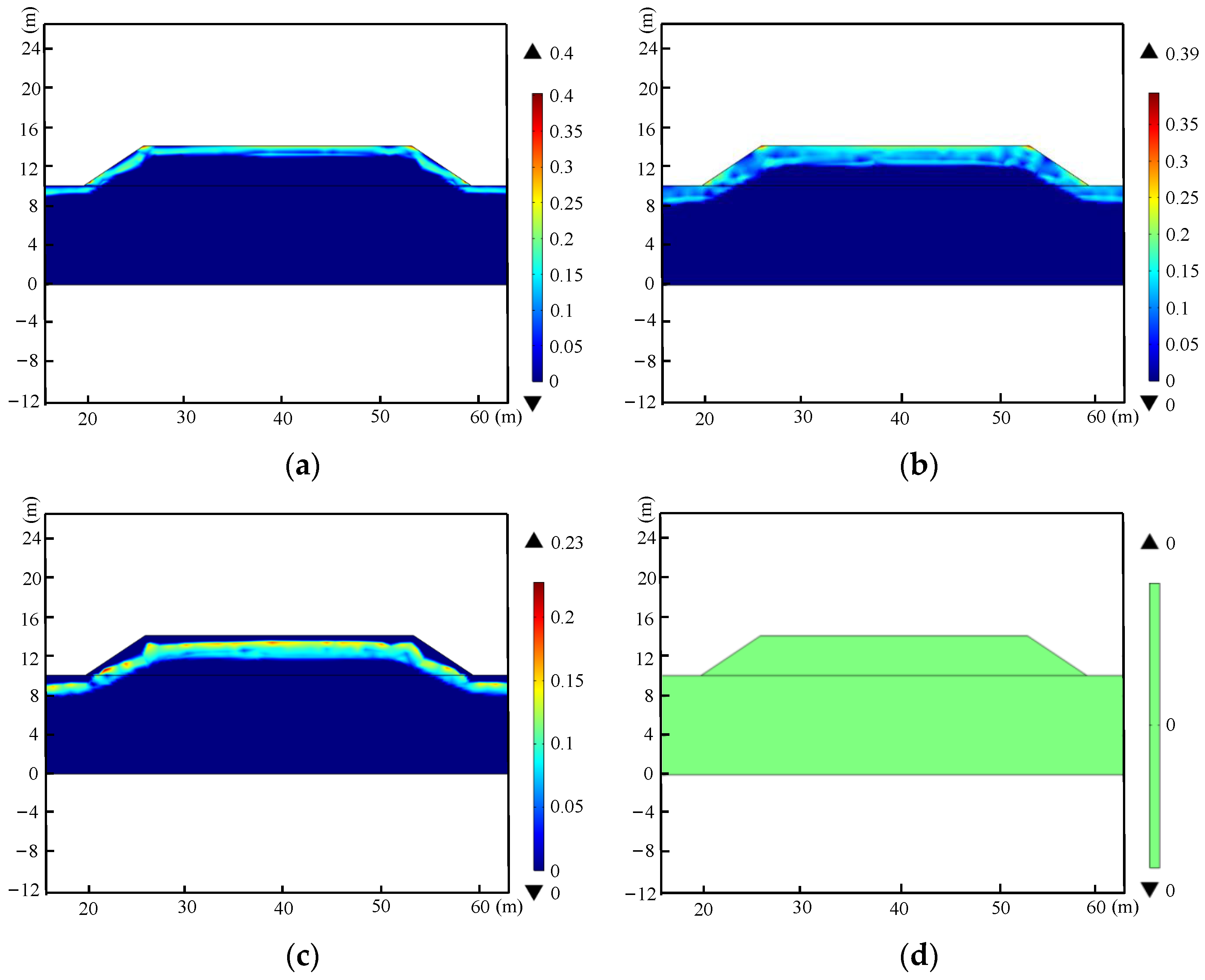
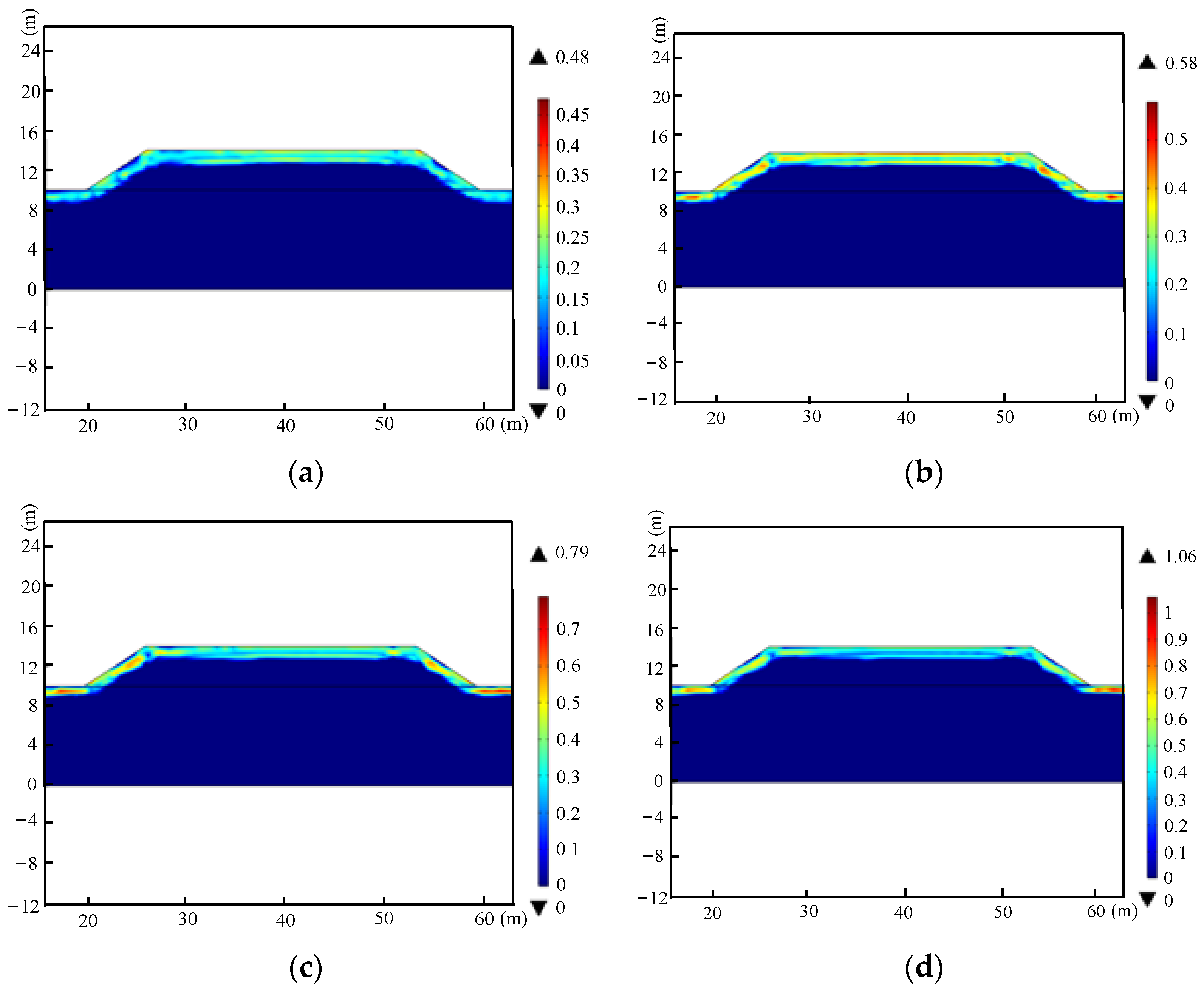
To assess annual variations in the moisture and ice content within the seasonally frozen roadbed, the moisture distributions on August 9th and ice content profiles on January 11th across the second, fourth, sixth, and eighth years post-construction were analyzed, utilizing water–heat coupling simulations, as shown in Figure 12 and Figure 13. The results indicated that over successive freeze–thaw cycles, both the surface and roadbed moisture and ice contents undergo continual redistribution, escalating with the cycle count. After eight years, the roadbed center ice content surged from 0% to 59.2%, while soil below a depth of ~2.5 m remained ice-free, aligning with the roadbed’s maximum freezing depth. Furthermore, by the eighth year, the water and ice content near the slope foot peaked at 86% and 106%, respectively, due to its encapsulation by frozen soil and heightened temperature sensitivity, facilitating omnidirectional water migration. The roadbed internal water also converged towards the slope foot under migration effects, leading to cumulative water content (excluding evaporation and drainage). It is inferred that prolonged freeze–thaw cycles will severely compromise the roadbed through frost heave and thaw settlement.
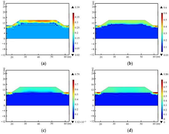
Figure 12.
Water content distribution in the roadbed after 8 years: (a) after 2 years, (b) after 4 years, (c) after 6 years, and (d) after 8 years.
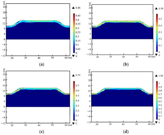
Figure 13.
Ice content distribution in the roadbed after 8 years: (a) after 2 years, (b) after 4 years, (c) after 6 years, and (d) after 8 years.
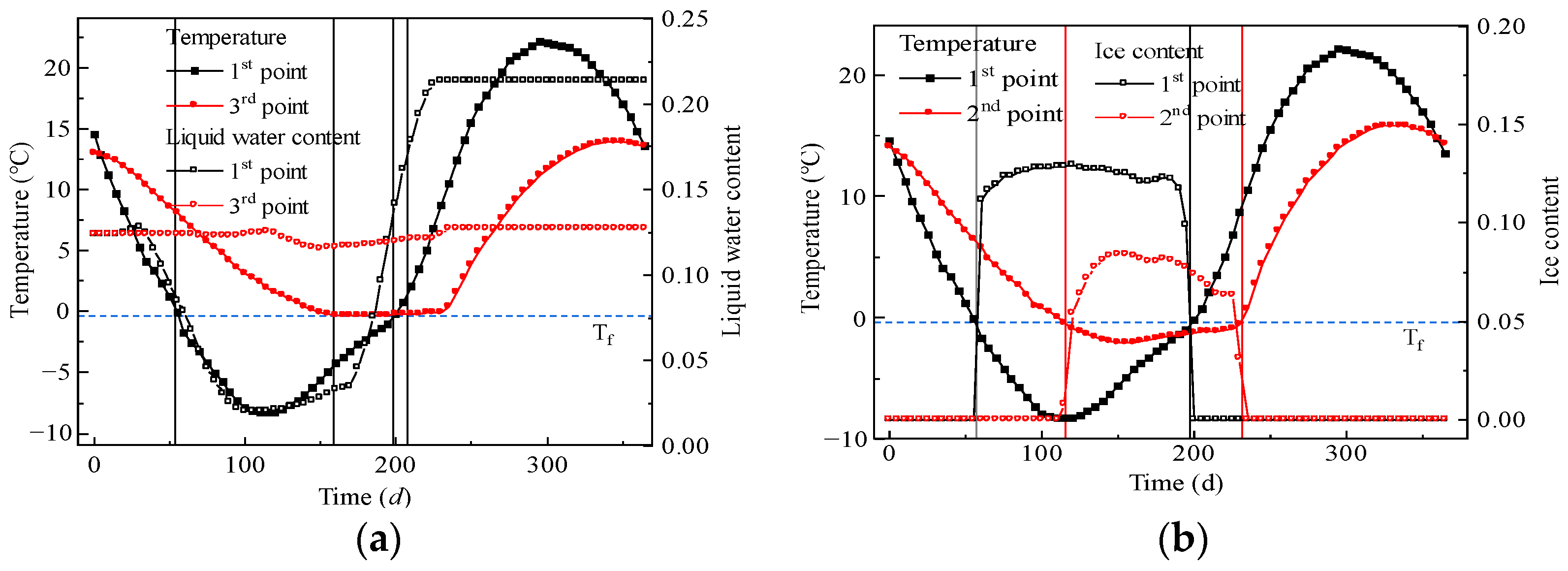
To investigate the water–heat interplay in roadbed soil, time history curves of the liquid water content and temperature, as well as ice content and temperature, were plotted and analyzed, as depicted in Figure 14. The results indicated that the liquid water content at point 1 began to decrease before the temperature reached the freezing point of the soil, and the liquid water at points 1 and 3 slightly increased during the freezing period due to water migration from unfrozen areas. After the temperature reached the freezing point, the ice content rapidly increased, whereas it decreased rapidly as the temperature reached the thawing point. However, the water content field had a slight lag compared to the temperature field. This is because ice is more sensitive to temperature, while liquid water can migrate as the temperature fluctuates.
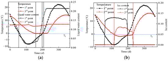
Figure 14.
Time history curves: (a) liquid water content and temperature and (b) ice content and temperature.
3.3. Deformation Analysis
3.3.1. Basic Equations for the Stress Field
The stress state of permafrost is complex, including the effects of gravity, external loads, pore water pressure, and frost heave. This investigation neglected the stress redistribution caused by external loads and pore water pressure and only analyzed the stress caused by frost heave. An elastic model was adopted, the soil was analyzed for elastic deformation, disregarding plastic and viscous deformations.
The equilibrium equation is:
The geometric equation is:
The present constitutive equation is:
During the calculation of permafrost strain, it is necessary to consider the phase change of water, the transient strain, and soil strain caused by water migration, which leads to:
During the process of water transforming into ice, the volume increases by 9%. The strain εv caused by water migration and the freezing phase change is:
As liquid water transforms into ice, the volume expands due to freezing and the migration of water from unfrozen zones, alongside in-pore water freezing. Assuming the volume of the soil particles remains constant, the porosity of the soil increases as the volume increases, caused by the water freezing into ice. Hence, frost heave can be quantified through porosity changes, expressed at time t as:
Then, the porosity at the time t + dt is:
The strain during soil freezing is:
Substituting Equations (23) and (24) into (25) yields:
3.3.2. Numerical Modeling
- (1)
- Calculation parameters
The mechanical parameters of the soil for the simulation are shown in Table 4. In the simulation, permafrost was treated as a frozen body composed of soil particles and ice, the elastic modulus of soil and ice were Es and Ei, respectively, and Poisson’s ratio of soil and ice was υs and υi, respectively. The content of the soil particles and ice was ns and ni, respectively. Thus, the equivalent elastic modulus and Poisson’s ratio of permafrost can be obtained as:
Table 4.
Mechanical parameters of the soil.
The elastic modulus of ice at different temperatures is shown in Table 5. A linear relationship, with a correlation coefficient R2 of 0.92, can be obtained through linear regression, as shown in Equation (29).
where T is the temperature of the ice and T* is the freezing point of the soil.
Table 5.
Elastic modulus of ice at different temperatures.
- (2)
- Boundary conditions
The roadbed’s GH bottom boundary was reinforced with fixed constraints, while its AH and FG side boundaries had roller support. The rest of the roadbed’s boundaries were free.
- (3)
- Roadbed freezing and thawing coefficient
The relationship between the freezing coefficient and the ice content was described using an empirical equation, as follows:
The equation includes empirical coefficients A, B, and C, which can be obtained from Table 6. The mass fraction ωI(x, y) of the ice content θI(x, y) is used to express their proportion relationship, as follows:
Table 6.
Empirical coefficients.
The thawing coefficient is mainly related to the water content, dry density, and porosity. This investigation used the water content method (ω method) for the calculation [26], and the empirical relationship between the thawing coefficient and water content can be obtained as follow:
where ωc represents the initial thawing water content of different soil types, and K1 is an empirical coefficient related to different soil types. The values of ωc and K1 are presented in Table 7.
Table 7.
Values of ωc and K1 of different soil types.
- (4)
- The deformation analysis steps
First, based on the established water–heat coupling model, the solid mechanics module was added, and the aforementioned water–heat coupling results were imported into the model through interpolation functions. Then, the thermal expansion interface was introduced into the solid mechanics interface, and the relevant parameters and boundary conditions were set. The thermal expansion coefficient was calculated using the secant method. When the temperature fell below the freezing point of the soil, the freezing coefficient was applied. Conversely, when the temperature exceeded the soil’s freezing point, the thawing coefficient was used. The thermal expansion coefficients of gravelly soil and powdery clay were converted into IF statement inputs based on Equations (30)–(32). Taking powdery clay as an example, the input expression is as follow:
where Tf is the freezing point of powdery clay, and Q1 and Q2 define the freezing and thawing coefficient functions of powdery clay. Finally, set the research type as the steady state for model calculations.
3.3.3. Results and Discussion
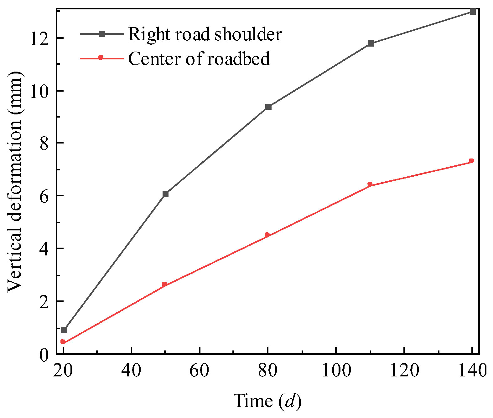
A study was conducted to investigate the deformation of the road and shoulder during freezing conditions, with displacement–time curves presented in Figure 15. It can be seen that by the 20th day, November’s onset saw a persistent decline in ambient temperature, leading to gradual roadbed soil expansion. Notably, the vertical deformation at the right shoulder exceeded that at the roadbed center. This is because the soil on both sides of the roadbed’s right shoulder is frozen and a large temperature gradient is formed during the freezing process. It freezes faster than the soil at the center of the roadbed. Therefore, the water in the roadbed soil migrates first to the shoulder, making the freezing and expansion of the soil at the shoulder more obvious. Furthermore, the period spanning from the 20th to 50th day marked a rapid phase of freezing and expansion, with substantial increases in frost heave. Subsequently, the rate of increase diminished on a monthly basis. By the 140th day, the maximum frost heave at the shoulder reached 13 mm, whereas the center of the roadbed experienced a maximum of 7.3 mm. This disparity in deformation between the shoulder and roadbed center will cause uneven deformation of the road.
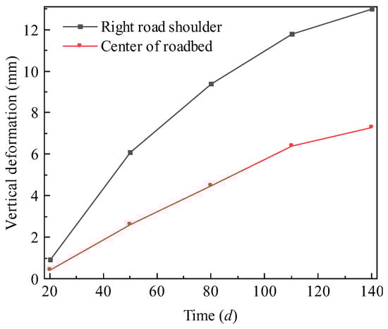
Figure 15.
Displacement versus time curve for the middle of the roadbed and the left shoulder during freezing.
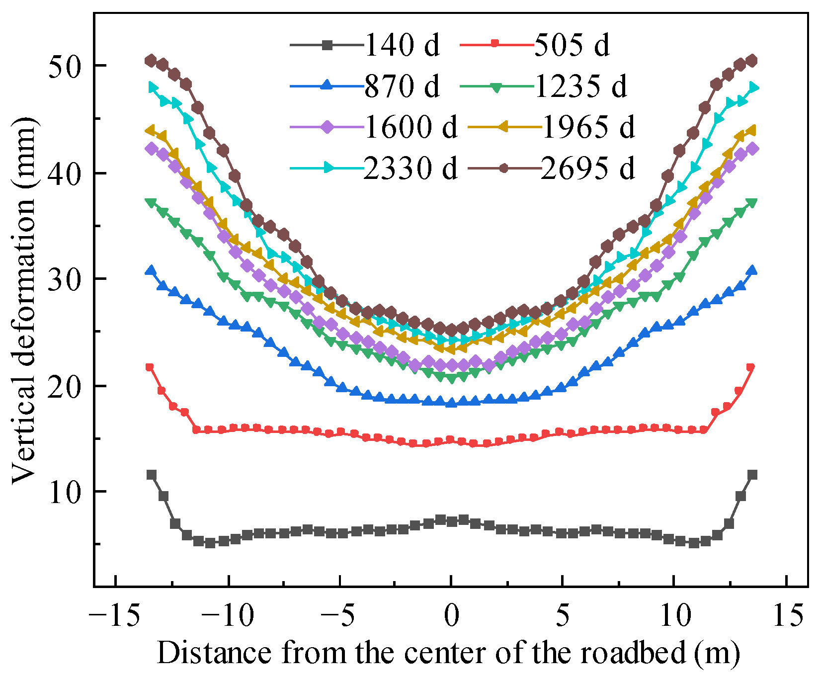
An analysis of frost heave deformation on 7 March, annually, was conducted, as depicted in Figure 16, revealing a symmetrical distribution of deformations along the transverse direction. Notably, the roadbed surface exhibited uneven deformation, resulting in a concave shape post-frost heave. Furthermore, the roadbed underwent continuous moisture redistribution due to the influence of water migration, with each freeze–thaw cycle contributing to water accumulation in the upper layers. Neglecting external factors, like drainage and evaporation, this accumulation exacerbated the frost heave deformation over time. By day 140, the shoulder experienced a peak frost heave of 11.7 mm, which increased to 50.5 mm over 7 years. Similarly, the road center attained a maximum frost heave of 7.3 mm on day 140, increasing to 25.2 mm in 7 years. In summary, if the roadbed fill becomes waterlogged, the higher moisture content leads to greater frost heave deformation, and uneven settlement on the roadbed surface will continue to worsen.
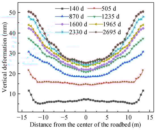
Figure 16.
Frost heave deformation of roadbed surface at different times.
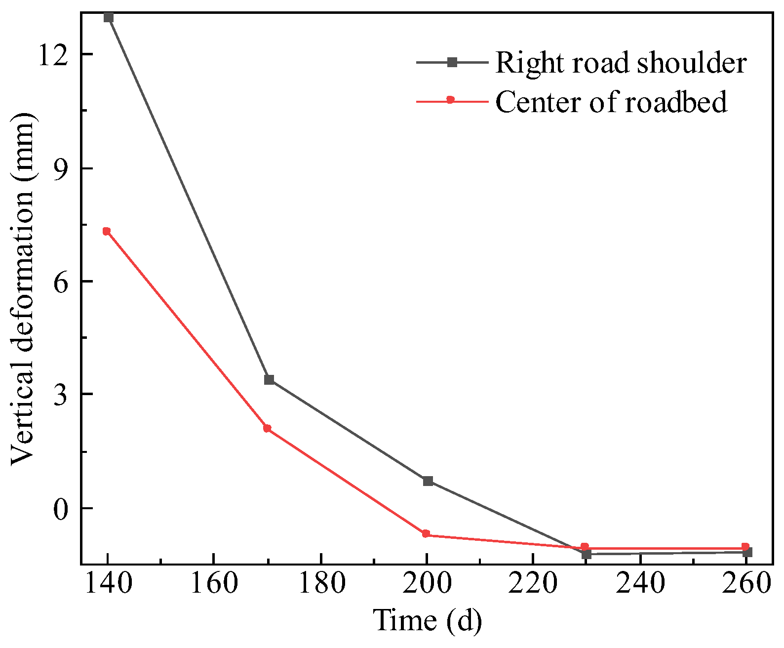
An analysis was conducted on the deformation of the roadbed and shoulders during the thawing period, and the displacement versus time curves are shown in Figure 17. It can be seen that after 140 days, the external environment transitioned to a warming phase, causing soil ice to gradually melt as temperatures rose. By the end of May, complete thawing of the roadbed permafrost led to substantial thaw settlement deformation, with the shoulders experiencing the most significant settlement. This is attributed to the preferential heating and thawing of shoulder soils, initiating rapid vertical displacement changes during the initial thaw period. During the thawing process, due to the deep-freezing depth during the freeze-up period, the thawing of the soil at the shoulders took a longer time. Additionally, the water content in the shoulder soil cannot be discharged in a timely manner, causing a larger thaw settlement amplitude, resulting in larger vertical displacement changes at the shoulder. Moreover, between days 140 and 170, there was a rapid phase of thaw settlement development, marked by a steep increase in the settlement growth rate. Subsequently, the thaw settlement rate gradually tapered off on a monthly basis, peaking at 1.2 mm on the 230th day, stabilizing thereafter. This trend stems from ice’s sensitivity to temperature; as temperatures rise, the soil ice content rapidly diminishes in the initial stages, leading to a corresponding decrease in frost heave deformation. When the ice completely thawed, water migration within the shallow subgrade layer caused an increase in water migration, leading to thaw settlement deformation. In summary, the difference in frost heave and thaw settlement deformation between the road center and shoulders can cause uneven deformation of the roadbed.
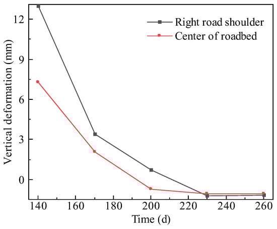
Figure 17.
Displacement versus time curve for the middle of the roadbed and the left shoulder during thawing.
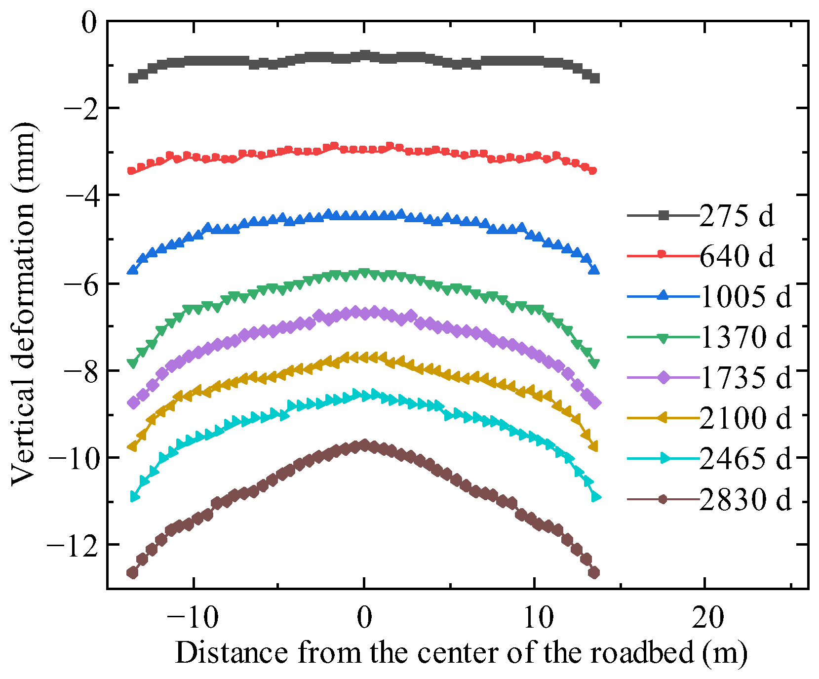
The thaw settlement on July 4th of each year was analyzed, as presented in Figure 18. It can be obtained that the thaw settlement deformation of the roadbed was symmetrically distributed along the transverse direction and there was uneven deformation on the roadbed surface, which presented a convex shape after thaw settlement deformation. Additionally, the roadbed underwent constant moisture redistribution due to the influence of water migration. Without considering external factors, such as drainage and evaporation, every freeze–thaw cycle caused water to accumulate on the upper and top surface of the roadbed. This gradual water accumulation enhances thaw settlement deformation over time. The shoulder exhibited a peak thaw settlement of 1.3 mm on the 275th day, escalating to 12.6 mm over 7 years. Comparatively, the road center peaked at 0.76 mm on the 275th day, reaching 9.67 mm after 7 years. Generally, waterlogged subgrade fills experience heightened thaw settlement with rising temperatures due to increased moisture content, exacerbating uneven settlement on the subgrade surface.
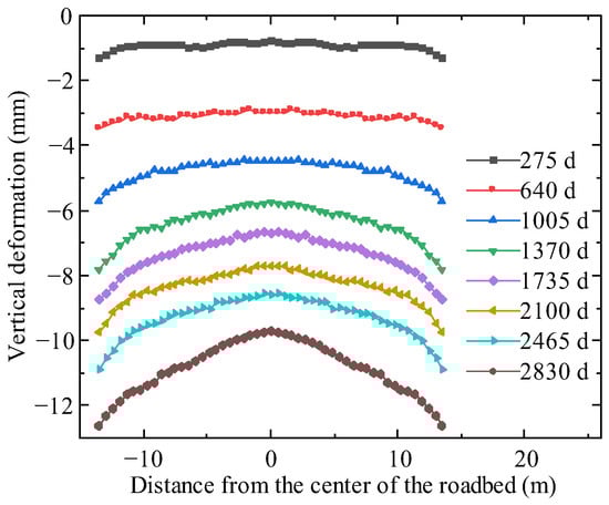
Figure 18.
Surface thaw settlement deformation of the roadbed at different times.
3.3.4. Discussion and Limitations
This investigation proposes a water–heat coupling model and implements a computational framework through the secondary development feature of COMSOL Multiphysics, to analyze the influence of water–heat coupling on roadbed deformation. However, this study also has some limitations, as follows:
- (1)
- A sensitivity analysis of the parameters has not been conducted yet. Initially, identify the dominant variables influencing the frost heave/thaw settlement. Subsequently, develop a multi-source data-driven model for evaluating and predicting the safety of seasonal permafrost roadbeds, with soil-sensitive parameters as controlled independent variables, and frost heave/thaw settlement as the target-controlled variables;
- (2)
- This investigation neglected the stress redistribution caused by external loads and pore water pressure and only analyzed the stress caused by frost heave, thus traffic load was not considered. Hence, it is necessary to incorporate dynamic traffic loads to further develop the water–heat coupling computational model under dynamic load conditions.
4. Conclusions
This study presented a combined theoretical and numerical investigation on the water–heat coupling characteristics of a seasonal permafrost roadbed. A water–heat coupling model was established and verified using the classic freeze–thaw test involving a soil column. Furthermore, an analysis of the frost heave and thaw-induced settlement deformations of the roadbed were conducted, focusing on their variations under temporal and thermal fluctuations. The key findings of this research can be summarized as follows:
- (1)
- A water–heat coupling mathematical model is established, of which the calculation is realized by using the secondary development module in the COMSOL software, thereby achieving the fully coupled numerical simulation of the temperature field and the moisture field. The accuracy of the model is verified by the classic freeze–thaw test involving a soil column. The simulation results are in good agreement with the test results, with an error of no more than 10%;
- (2)
- During the freezing and thawing process of the soil, the temperature distribution along the soil column direction is approximately linear, while the water migrates from the positive temperature zone to the negative temperature zone, with the maximum migration amount reaching 20% of the water content. Moreover, the balance of the water field lags behind that of the temperature field;
- (3)
- The duration of the soil freezing period is 4 months, with the maximum freezing depth of the roadbed being 2.5 m and that of the road shoulder being 2 m. After thawing, the water content in the shallow layer of the roadbed increases compared to the initial water content, leading to a decrease in soil strength;
- (4)
- After experiencing multiple freeze–thaw cycles, significant deformation occurs in the roadbed. In the first year, the vertical frost heave deformation of the roadbed is 6 mm, resulting in a concave-shaped road surface; the vertical thaw settlement deformation of the roadbed reaches 1.2 mm, resulting in a convex-shaped road surface. By the seventh year, the maximum frost heave can reach 51 mm, and the maximum thaw settlement can reach 13 mm.
Author Contributions
Conceptualization, B.L., W.Z. and S.L.; methodology, B.L. and W.Z.; software, B.L. and Z.X.; formal analysis, B.L. and Y.S.; investigation, Z.X. and Y.S.; resources, W.Z. and S.L.; data curation, M.D.; writing—original draft preparation, B.L. and M.D.; writing—review and editing, S.L. All authors have read and agreed to the published version of the manuscript.
Funding
This research was funded by the Fundamental Research Funds for the Central Universities (N180104013, Shengang Li) and the China Scholarship Council (202206080043, Bo Lu).
Data Availability Statement
Data will be made available on request.
Conflicts of Interest
Author Zhikang Xia was employed by the company The Construction Engineering Company of City Group. The remaining authors declare that the research was conducted in the absence of any commercial or financial relationships that could be construed as a potential conflict of interest.
References
- Wu, G.; Xie, Y.; Wei, J.; Yue, X. Freeze-thaw erosion mechanism and preventive actions of highway subgrade soil in an alpine meadow on the Qinghai-Tibet Plateau. Eng. Fail. Anal. 2023, 143, 106933. [Google Scholar] [CrossRef]
- Roh, H.J. Developing a risk assessment model for a highway site during the winter season and quantifying the functional loss in terms of traffic reduction caused by winter hazards conditions. J. Transp. Eng. Part A Syst. 2022, 148, 04022036. [Google Scholar] [CrossRef]
- Cai, H.; Hong, R.; Xu, L.; Wang, C.; Rong, C. Frost heave and thawing settlement of the ground after using a freeze-sealing pipe-roof method in the construction of the Gongbei Tunnel. Tunn. Undergr. Space Technol. 2022, 125, 104503. [Google Scholar] [CrossRef]
- Derk, L.; Unold, F. Effect of temperature gradients on water migration, frost heave and thaw-settlement of a clay during freezing-thaw process. Exp. Heat Transf. 2023, 36, 585–596. [Google Scholar] [CrossRef]
- Huang, X.; Rudolph, D.L.; Glass, B. A Coupled Thermal-Hydraulic-Mechanical Approach to Modeling the Impact of Roadbed Frost Loading on Water Main Failure. Water Resour. Res. 2022, 58, e2021WR030933. [Google Scholar] [CrossRef]
- Zheng, Z.; Bao, Z.; Yang, J.; Cui, M.; Ma, X.; Li, Y. The products transformation and leaching behavior in solidified cement matrices under the coupling actions of “water-heat-chemistry. Constr. Build. Mater. 2022, 323, 126565. [Google Scholar] [CrossRef]
- Sun, W.; Fish, J.; Leng, Z.; Ni, P. PD-FEM chemo-thermo-mechanical coupled model for simulation of early-age cracks in cement-based materials. Comput. Methods Appl. Mech. Eng. 2023, 412, 116078. [Google Scholar] [CrossRef]
- Taber, S. The mechanics of frost heaving. J. Geol. 1930, 38, 303–317. [Google Scholar] [CrossRef]
- Everett, D.H. The thermodynamics of frost damage to porous solids. Trans. Faraday Soc. 1961, 57, 1541–1551. [Google Scholar] [CrossRef]
- Harlan, R.L. Analysis of coupled heat-fluid transport in partially frozen soil. Water Resour. Res. 1973, 9, 1314–1323. [Google Scholar] [CrossRef]
- Taylor, G.S.; Luthin, J.N. A model for coupled heat and moisture transfer during soil freezing. Can. Geotech. J. 1978, 15, 548–555. [Google Scholar] [CrossRef]
- Zhan, Y.; Zhao, M.; Lu, Z.; Liu, G.; Yao, H. Study on water–heat coupling migration law and frost heave effect of soil slope in seasonal frozen regions during groundwater recharge. Environ. Earth Sci. 2023, 82, 401. [Google Scholar] [CrossRef]
- Booshehrian, A.; Wan, R.; Su, X. Hydraulic variations in permafrost due to open-pit mining and climate change: A case study in the Canadian Arctic. Acta Geotech. 2020, 15, 883–905. [Google Scholar] [CrossRef]
- Mihara, K.; Kuramochi, K.; Toma, Y.; Hatano, R. Effect of water movement in frozen soil on long-term hydrological simulation of Soil and Water Assessment Tool in cold climate watershed in Hokkaido, Japan. Soil Sci. Plant Nutr. 2024, 70, 160–173. [Google Scholar] [CrossRef]
- Yin, X.; Liu, E.; Song, B.; Zhang, D. Numerical analysis of coupled liquid water, vapor, stress and heat transport in unsaturated freezing soil. Cold Reg. Sci. Technol. 2018, 155, 20–28. [Google Scholar] [CrossRef]
- Li, Z.; Liu, X.; Sun, Y.; Jiang, X. Numerical simulation of frost heaving damage of earth-rock dam berms in cold regions with thermo-hydro-mechanical coupling. Cold Reg. Sci. Technol. 2024, 223, 104207. [Google Scholar] [CrossRef]
- Lu, D.; Meng, F.; Zhou, X.; Zhuo, Y.; Gao, Z.; Du, X. A dynamic elastoplastic model of concrete based on a modeling method with environmental factors as constitutive variables. J. Eng. Mech. 2023, 149, 04023102. [Google Scholar] [CrossRef]
- Lu, D.; Liang, J.; Du, X.; Ma, C.; Gao, Z. Fractional elastoplastic constitutive model for soils based on a novel 3D fractional plastic flow rule. Comput. Geotech. 2019, 105, 277–290. [Google Scholar] [CrossRef]
- Zhang, H.; Zhang, J.; Zhang, Z.; Zhang, M.; Cao, W. Variation behavior of pore-water pressure in warm frozen soil under load and its relation to deformation. Acta Geotech. 2020, 15, 603–614. [Google Scholar] [CrossRef]
- Deng, Q.; Liu, X.; Zeng, C.; He, X.; Chen, F.; Zhang, S. A freezing-thawing damage characterization method for highway subgrade in seasonally frozen regions based on thermal-hydraulic-mechanical coupling model. Sensors 2021, 21, 6251. [Google Scholar] [CrossRef]
- Botkin, N.D.; Brokate, M.; El Behi-Gornostaeva, E.G. One-phase flow in porous media with hysteresis. Phys. B Condens. Matter 2016, 486, 183–186. [Google Scholar] [CrossRef]
- Biryukov, A.B.; Ivanova, A.A. Diagnosis of temperature conditions in metals when heated in continuous furnaces. Metallurgist 2018, 62, 331–336. [Google Scholar] [CrossRef]
- Tian, K.; Yang, A.; Nie, K.; Zhang, H.; Xu, J.; Wang, X. Experimental study of steady seepage in unsaturated loess soil. Acta Geotech. 2020, 15, 2681–2689. [Google Scholar] [CrossRef]
- Xu, X.; Wang, J.; Zhang, L. Permafrost Physics; Science Press: Beijing, China, 2001; pp. 75–98. (In Chinese) [Google Scholar]
- Ma, Z.; Lin, C.; Zhao, H.; Yin, K.; Feng, D.; Zhang, F.; Guan, C. Numerical Simulations of Failure Mechanism for Silty Clay Slopes in Seasonally Frozen Ground. Sustainability 2024, 16, 1623. [Google Scholar] [CrossRef]
- Vanmarcke, E. Random fields: Analysis and Synthesis; MIT Press: Cambridge, MA, USA, 1983. [Google Scholar]


Disclaimer/Publisher’s Note: The statements, opinions and data contained in all publications are solely those of the individual author(s) and contributor(s) and not of MDPI and/or the editor(s). MDPI and/or the editor(s) disclaim responsibility for any injury to people or property resulting from any ideas, methods, instructions or products referred to in the content. |
© 2024 by the authors. Licensee MDPI, Basel, Switzerland. This article is an open access article distributed under the terms and conditions of the Creative Commons Attribution (CC BY) license (https://creativecommons.org/licenses/by/4.0/).