Optimization of Ground Source Heat Pump System Based on TRNSYS in Hot Summer and Cold Winter Region

Abstract

A cooling tower-assisted ground source heat pump system is proposed to solve the problem of soil heat accumulation in areas with hot summers and mild winters. TRNSYS is used to establish the simulation model of the ground source heat pump system. Taking the ground source heat pump demonstration project in Nanchang City as the research object, the operation effect of the ground source heat pump is simulated and analyzed. The key parameters of the optimization system are proposed, and the operation time of the cooling tower is controlled. The optimization results show that the cooling tower can not only improve the system performance in a short time but also enable long-term stable and efficient operation of the refrigeration system, the compound ground source heat pump system optimized by the cooling tower has almost no soil heat accumulation, and the system performance has been improved. The optimal running time of the cooling tower is 3216~4344 h and 5424~6696 h, and the system running effect is the best at this time. The research results can provide a theoretical basis for the optimal design of the cooling tower auxiliary ground source heat pump system.

1. Introduction

In the context of energy conservation and emission reduction in China [1,2,3], ground source heat pump technology has received increasing attention due to its energy-saving and environmental protection characteristics, and it has developed rapidly in recent years. In areas with hot summers and mild winters, due to the greater demand for cooling load from buildings than for heating load, the heat released to the ground by the ground source heat pump system is much higher than the heat absorbed, causing the soil temperature to rise and resulting in “heat accumulation”. This leads to an increase in the required energy consumption of the heat pump unit, making the system even less able to meet the cooling demand [4]. Research has found that to achieve the same cooling effect, for every 1 °C increase in average soil temperature, energy consumption will increase by 3% to 4% [5]. If the problem of soil temperature rise is not taken seriously, the soil temperature in the buried pipe heat exchange area will rise even higher, which will cause the operation of the system to deteriorate significantly and even lead to high inlet water temperature in the buried pipe, making the heat pump unit unable to operate normally and stably. In severe cases, it may cause shutdown and other failures [6,7].

In order to solve the problem of soil thermal accumulation, relevant scholars have conducted extensive research. Liu et al. [8] compared a traditional geothermal heat pump (GSHP) and cooling tower coupled geothermal heat pump system (HGHP), and their simulation found that the performance coefficient of the HGHP increased by 7.12%, the energy consumption decreased by 6.4%, and the outlet temperature of buried pipes was below 32 °C over ten years of operation. Qiu et al. [9] established a dynamic thermodynamic model of the PVT-GSHP system based on TRNSYS and used the genetic algorithm to optimize the optimal buried pipe length corresponding to different PVT collector regions, and the optimized matching annual average temperature of thermal reservoirs in the interior of the life cycle met the requirements of geothermal balance. Cui et al. [10] proposed different optimization control strategies for parallel and series ground source heat pump auxiliary cooling towers, respectively. Xie Yiwei et al. [11] proposed a group control strategy based on multi-step load prediction and applied it to a hybrid ground source heat pump system to obtain the optimal MAE and MAPE, which can reduce the degradation of energy performance caused by soil heat accumulation. Yang et al. [12] studied a ground source heat pump system, which is equipped with dual cooling towers and traditional composite parallel ground source heat pumps in the cooling dominant area, replacing buried pipe heat exchangers to alleviate soil heat accumulation in summer. Deng Fengqiang et al. [13] considered the on-site hydrogeological conditions of ground source heat pump systems and proposed using the heat from seasonal groundwater to supplement thermal imbalances. Chen Dajian et al. [14] chose TRNSYS18 software to establish a cooling tower-assisted ground source heat pump composite system, proposed a control strategy for the alternating operation of the cooling tower day and night, and compared the control strategies of the cooling tower under different typical climate zones and operating conditions. Research has found that intermittent operation and day–night alternation operation of cooling towers can better control the auxiliary heat dissipation of cooling towers and better balance the ground temperature field in the heat exchange area. Fan Qi et al. [15] studied the time effect of the spacing between the holes of buried heat exchangers and the 10-year operation of ground source heat pump systems. They found that adopting an operation mode where the summer cooling and winter heating operation times were as equal as possible and the summer recovery period was extended could eliminate the heat imbalance generated in the rock and soil mass. Wang Chuang [16] took a building in Beijing as the research object, established a simulation model using TRNSYS software, and proposed a new optimization control strategy. Seung-Hoon Park et al. [17] proposed a loop configuration and operation strategy for a serially connected HyGSHP system. Through quantitative analysis, they found that factors such as the ground temperature, total required length of BHEs, and heat pump COPs have a mitigating effect on long-term geothermal imbalance, and they verified the validation of the proposed system. Chen et al. [18] explored a ground source heat pump system that is integrated with a cooling tower for auxiliary heat dissipation. They analyzed this auxiliary heat dissipation approach by controlling the cooling tower with a predetermined load ratio. The results show that when the cooling tower is connected in series with the soil source heat pump system, the optimal heat dissipation method for controlling the start and stop of the cooling tower is achieved when the load ratio is 0.55. After 10 years of operation, the soil temperature increases by 0.4 °C, while the system COP remains at 5.8. The above research focuses on the operating mode and strategy of the system, and it does not involve key parameters.

This paper introduces a novel approach by proposing a cooling tower-assisted ground source heat pump system specifically designed to address the soil thermal accumulation problem prevalent in hot summers and mild winters regions. Using the ground source heat pump demonstration project in Nanchang City as a case study, we establish a model of the GSHP system employing TRNSYS software. The paper emphasizes design and operational optimization, selecting the operation time of the cooling tower as a critical parameter influencing system performance. This unique identification of operational time as a key parameter, coupled with our focus on maintaining stable soil temperatures, sets our work apart from existing studies. Our proposed system scheme is designed to ensure that the average soil temperature does not rise, improving the operational efficiency of the GSHP. Through this innovative framework, we aim to provide valuable reference and guidance for the practical implementation of ground source heat pump energy-saving technologies, promoting their widespread application in similar climatic conditions.

2. Building and Load Calculation Model

In the study of building energy systems, load calculation is a crucial step. To accurately simulate and assess the overall energy efficiency of a building and the effectiveness of selected systems, it is essential to establish detailed models of the building and its load calculation. This section will discuss in detail the building load calculation model used in this research, including an overview of the building, the system simulation modules, and the building load simulation.

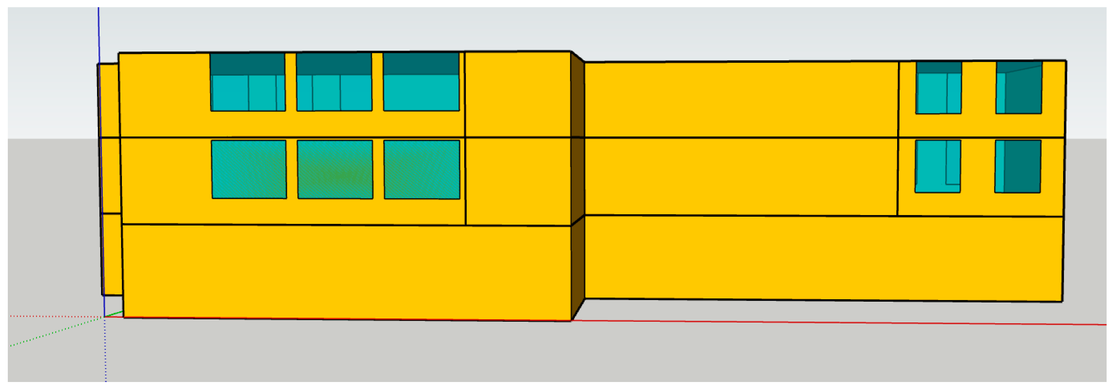
2.1. Architectural Overview

This building is an integrated building for scientific research and offices in Nanchang City with three floors above ground, 3.25 m for the first floor, 3 m for the second floor, 2.9 m for the third floor, 9.15 m for the total floor height, 1100 m² for the building area and 759 m² for the air conditioning area. Two independent ground source heat pump central air conditioning systems are designed and installed: one ground source heat pump (GSHP) system on the first floor, utilizing extracted groundwater as the heat source, and a ground-coupled heat pump (GCHP) system on the second and third floors, utilizing buried pipes for heat exchange. The GCHP system adopts vertical buried pipe mode, and 16 heat exchange holes with a depth of 100 m are arranged in a square of 4 m × 4 m at the green belt 4 m to the east of the building. Among them, eight single-U heat exchange holes and eight double-U heat exchange holes are distributed as shown in Figure 1. Moreover, the connections for the borehole heat exchangers are configured in a parallel arrangement, where each borehole is connected directly to the manifold. The GSHP system is equipped with two pumping and recharge wells on the north side of the building, and the two wells can be used interchangeably on a regular basis.

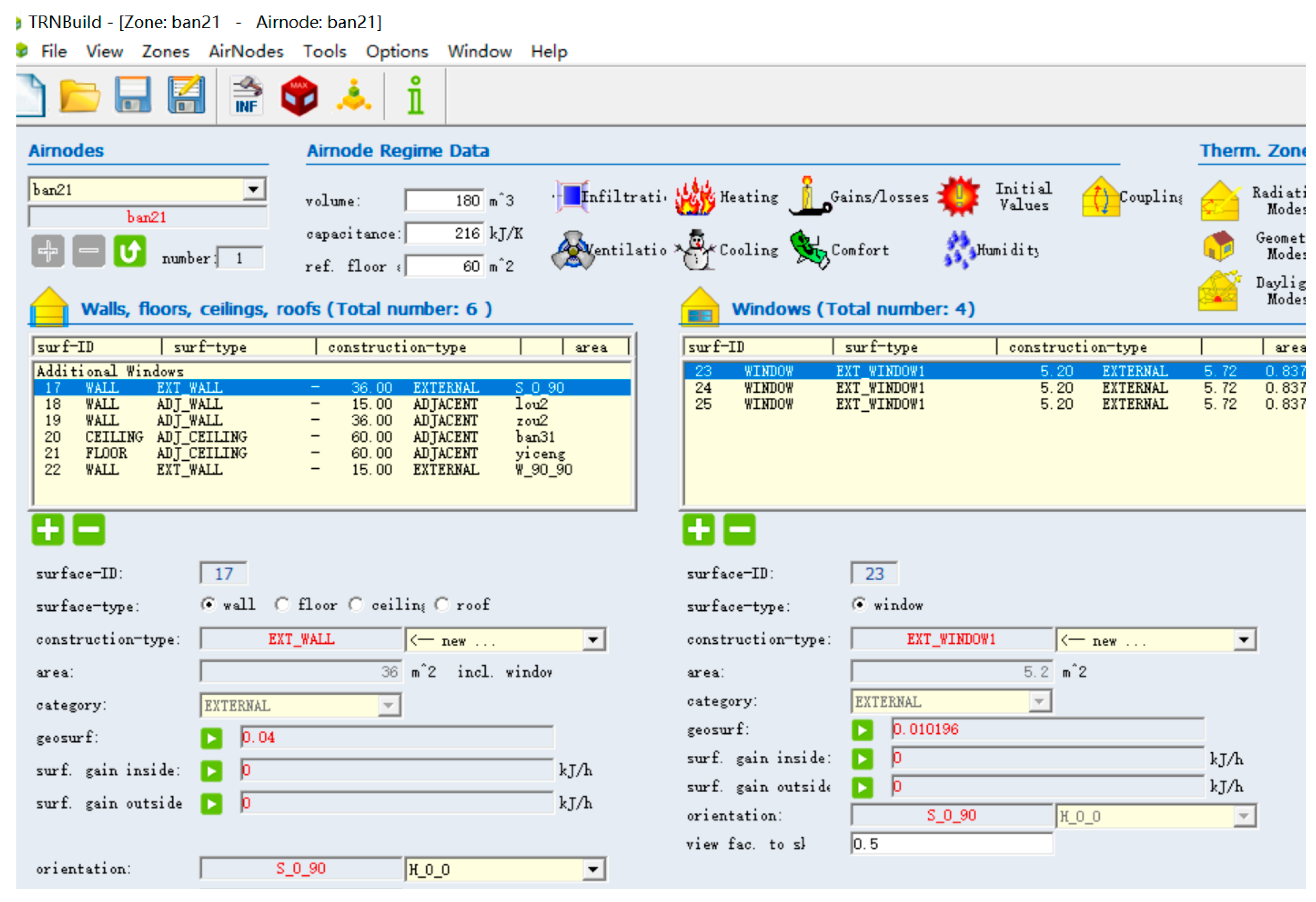
2.2. System Simulation Module

TRNSYS software is a transient system simulation program that was initially developed by the Solar Energy Laboratory of the University of Wisconsin-Madison in the United States and gradually improved by some European institutions (CSTB, TRANSSOLAR). This article establishes a simulation model of a ground source heat pump system using TRNSYS18 as the platform. Based on the actual situation of the building, it selects the corresponding module, sets the parameter values, establishes connections, and builds a simulation system. The simulation system mainly uses the following modules: load reading module, water pump module, heat pump unit module, and buried pipe heat exchanger module. The details of all design modules can be found in

Table 1. TRNSYS module details.

Module Name	Module Number	Module Description
Multi-area building	Type56	Call the “bui” building model file edited by TRNBuild
Burthen	Type682	Building load treatment
Heat pump	Type225	Water–water modular heat pump unit
Buried pipe heat exchanger	Type557a	U-type buried pipe, vertical buried pipe heat exchanger
Fixed frequency pump	Type114	Circulating water pump, frequency conversion operation
Weather data read	Type15-2	Read the weather data file in the standard format
Free-format data reads	Type9e	Data at the beginning of the first behavior simulation, used to read the load data files
Control signal	Type14	Heat pump unit cooling and heating working condition time setting
Current diverter	Type11f	Fluid shunt device
Commingler	Type11h	Fluid mixing device
geotemperature	Type77	Surface temperature output
Data output	Type65a	Graphic output module with output files
calculator	Unit	Customstom formula for output

.

2.3. Building Load Simulation

When the ground source heat pump system starts up and heats the building, the cold and heat load of the heat pump unit will change with the change in the building load. Accurately grasping the dynamic load of buildings throughout the year not only enables the efficient operation of heat pump units but also serves as an external file for TRNSYS system simulation calls, improving the accuracy of system simulation. Therefore, it is necessary to conduct a dynamic simulation of buildings throughout the year.

When calculating the annual dynamic load of the building, a 3D model of the building is first established using SketchUp2018 software. A new 3D Building project is created to import the building model containing the geometry and structure information (.idf file) and the project weather (.tm2 file). The building envelope structure, indoor design parameters, heating and cooling times, and other relevant parameters are then set in TRNBuild. The sensible heat load and latent heat load of each hot zone are outputted, and finally, the annual load of the building is calculated using the calculator module. The annual dynamic load calculation model is shown in Figure 2.

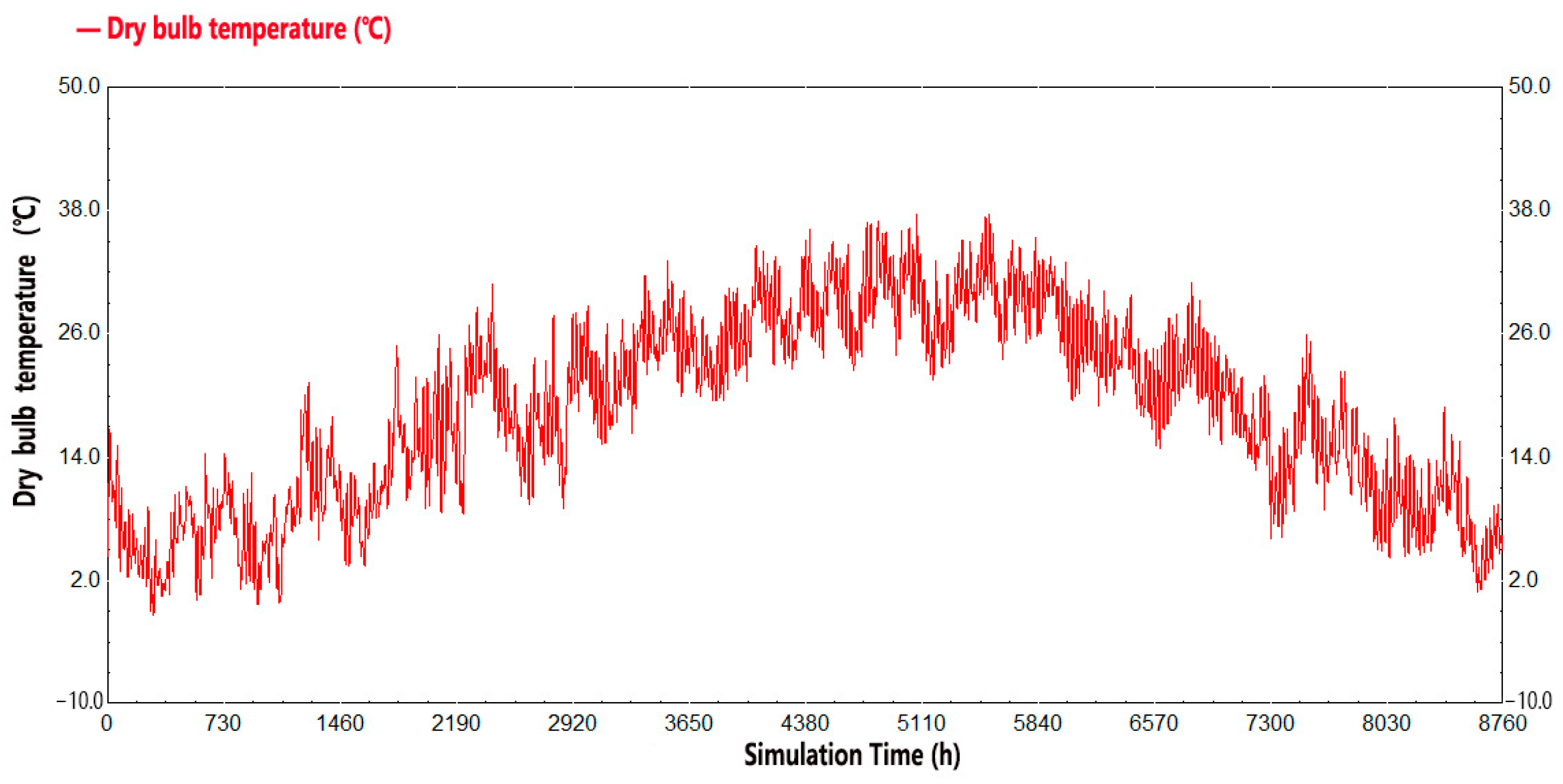
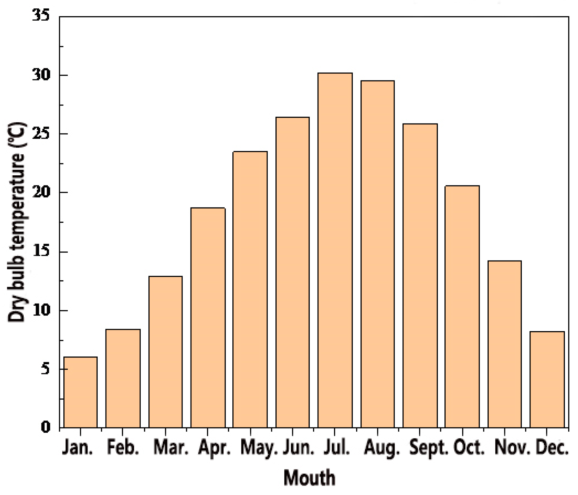
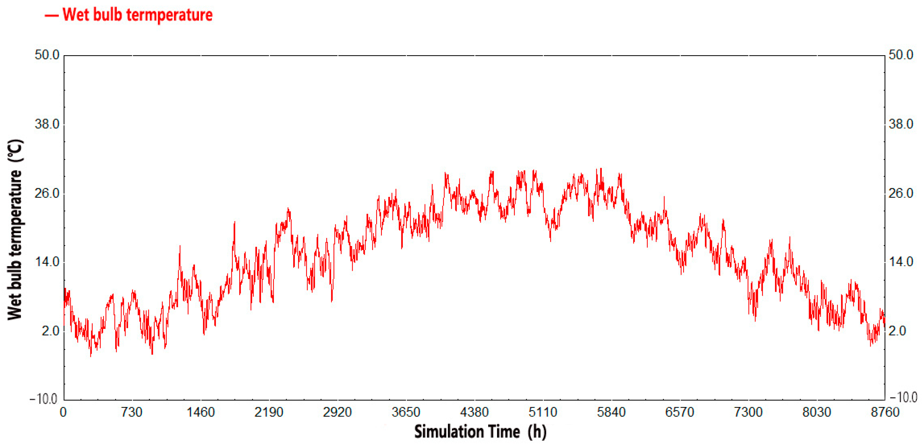
2.3.1. Analysis of Building Meteorological Parameters

Because meteorological parameters affect the required cooling load and heat load of building air conditioning, they also affect the operation of the building’s air conditioning system. We simulated these conditions in TRNSYS based on the meteorological file in TMY2 format exported from the Meteonorm8.0 meteorological database software. By loading the TMY2 format meteorological file into the simulation software to output meteorological parameters, the annual hourly meteorological parameters of the project location were obtained, forming a typical outdoor meteorological condition for the project area for one year. A typical meteorological year refers to selecting the monthly average of the past 10 years as the benchmark and selecting the average of each month in the past 10 years from the data as the typical meteorological year [19]. By loading meteorological data files into simulation software, various meteorological parameters of typical meteorological years in the project area are obtained, and then some parameters are selected for analysis.

Outdoor dry bulb temperature is an important factor affecting the intensity of cold and heat load. The hourly outdoor dry bulb temperature and monthly average outdoor dry bulb temperature for a typical meteorological year in the project area are shown in Figure 3 and Figure 4, respectively. Figure 3 shows that the highest temperature in the project area is 37.7 °C in July, and the lowest temperature is −1.35 °C in January; Figure 4 shows that the average outdoor temperature in July was 30.2 °C, while the average outdoor temperature in January is 6.1 °C. From Figure 3 and Figure 4, it can be seen that the months with a daily average outdoor temperature above 20 °C are from May to October, and the months with a daily average outdoor temperature below 10 °C are from December to February.

As mentioned above, according to an outdoor weather temperature analysis of outdoor weather parameters in the project area, combined with system control and actual needs, the opening time of building air conditioning is obtained. The cooling season runs from 15 May to 6 October, and the heating season runs from 14 November to 14 March. This building is an office building. According to the load characteristics of urban office buildings, the control conditions of air conditioning in cooling and heating periods are generally set at 8:30 to 17:30 every day as the start-up operation time.

2.3.2. Project Overview

The simulated building has three floors. The building model is established by SketchUp software. The boundary condition matching of all hot zones of the building is set in this software. By setting the size parameters of hot zones and building rooms, the 3D physical model of the building is obtained as shown in Figure 5. This is a simulation of the ground source heat pump system in the buried pipe ground source heat pump part, that is, the annual load calculation for the second and third floors of the building.

• Thermal parameters of envelope structure

The simulated building objects are the second floor and the third floor of the office building. The thermal parameters of the building’s internal and external walls, roof and floor are shown in

Table 2. Thermal parameters of the envelope structure.

Type of Enclosure Structure	Thickness/m	Heat Transfer Coefficient/w (m−2·k)
Interior wall	0.12	1.88
Exterior wall	0.300	1.96
Floor slab	0.325	1.46
Floor board	0.365	0.589
Rooftop	0.285	0.7

.

2.

Interior design parameters

The winter indoor air conditioning design temperature is 20 °C, and the relative humidity is 50%; The design temperature for indoor air conditioning in the summer is 26 °C, the relative humidity is 60%, the lighting power density is 9 W/m², and the electrical power density is 15 W/m [20]. The per capita occupancy area of the office is set at 10 m²/person, and the per capita fresh air volume is 30 m³/h. The office staff occupancy rate, office lighting utilization rate, and office equipment utilization rate are shown in Figure 6.

3.

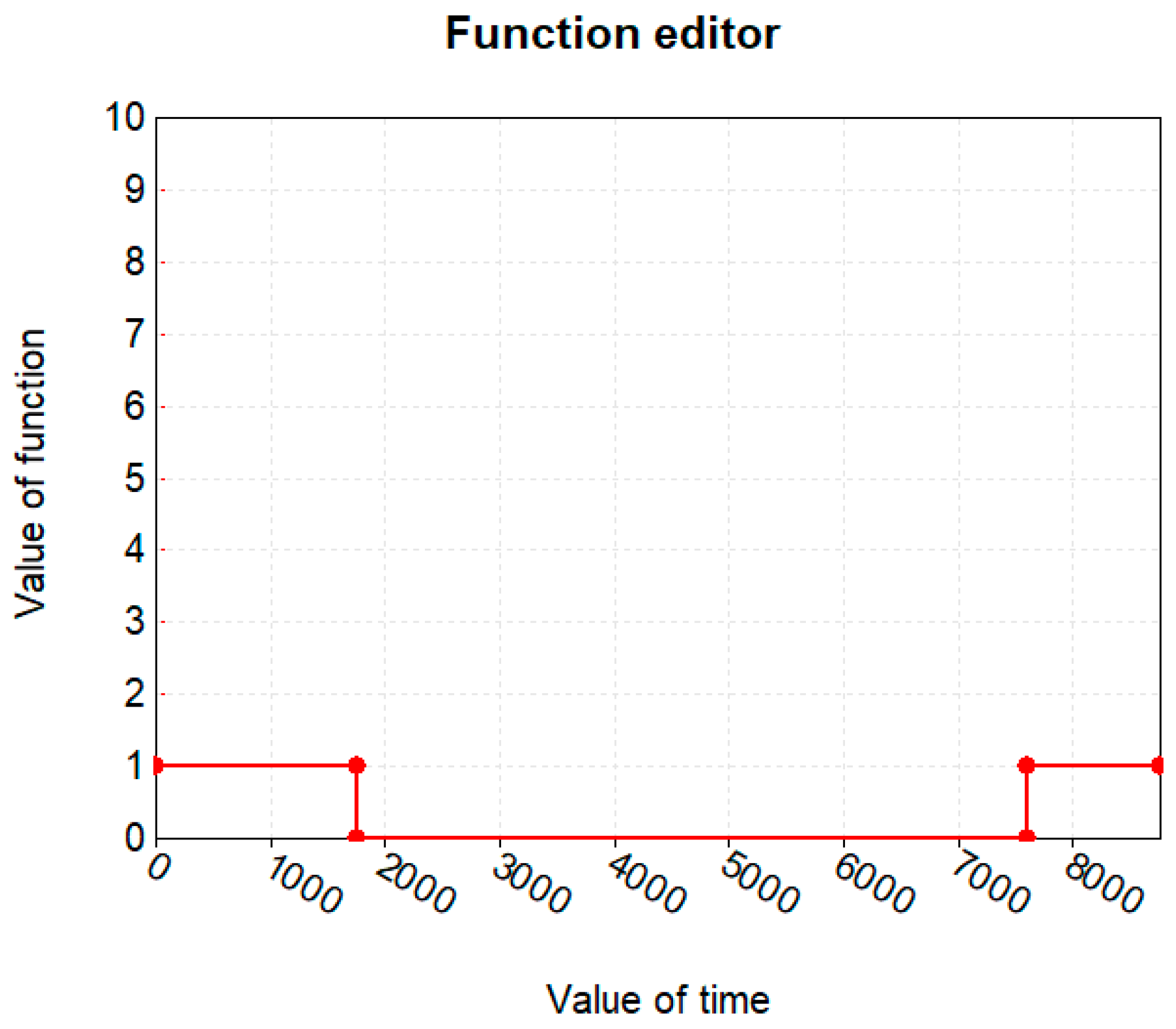
Building heating and cooling time

The office air conditioning system operation time is weekdays in 8:30~17:30, not running on weekends; summer air conditioning in 15 May~6 October, a total of 145 days; winter heating period for 14 November~14 March, a total of 120 days.

The building envelope information, interior design parameters and control settings are integrated to establish a dynamic load calculation platform in TRNBuild, as shown in Figure 7.

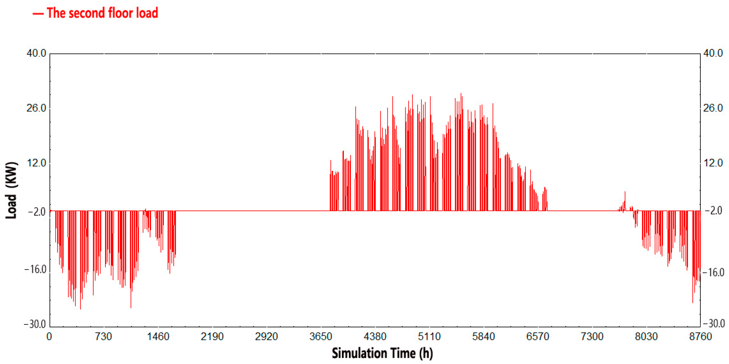
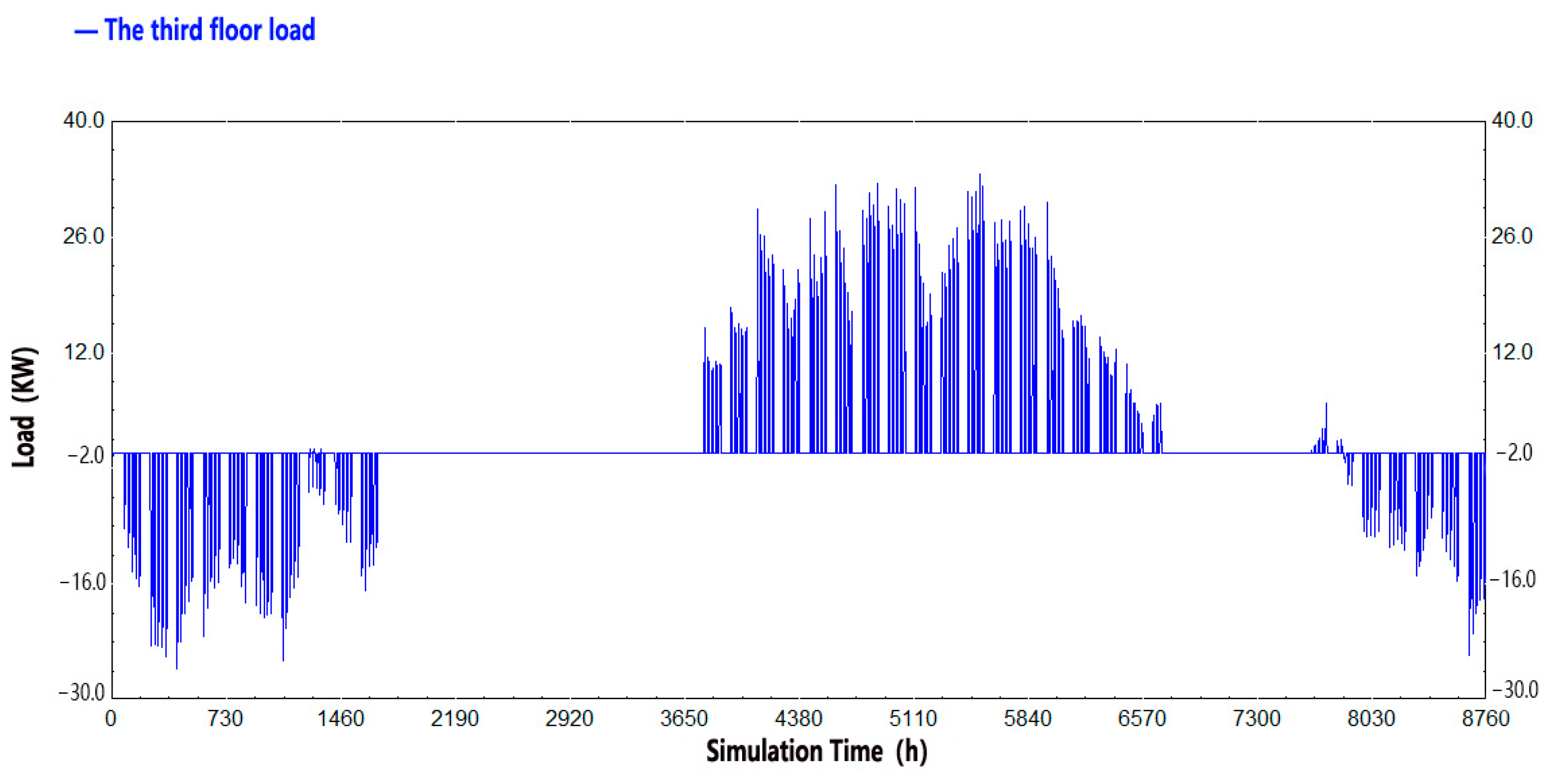
2.3.3. Load Simulation

The calculation platform of building load dynamic simulation established in the Simulation Studio program of TRNSYS software can calculate the hourly load of the second and third floors of buildings throughout the year. The results are shown in Figure 8 and Figure 9, where the heat load is negative and the cold load is positive. Through simulation, it is found that the maximum hourly cooling load of the second floor of the building is 30 kW at 5530 h, the maximum hourly heating load is 25.14 kW at 421 h, the cumulative cooling load is 14,198 kWh, the annual cumulative heating load is 7440 kWh, the maximum hourly cooling load of the third floor of the building is 33.78 kW at 5330 h, and the maximum hourly heating load is 26.22 kW at 421 h. The cumulative cooling load is 15,831 kWh and the annual cumulative heat load is 7899 kWh. The cumulative cooling load of the second and third floors of the building is 30,029 kWh, the cumulative heat load is 15,339 kWh, and the ratio of cumulative cold and heat demand of the second and third floors of the building is 1.96:1. This area is hot in summer and cold in winter, so the heating time in winter is less than the cooling time in summer, so the required heat load is much less than the cooling load.

3. Research on Prospective Prediction Model of Ground Source Heat Pump System

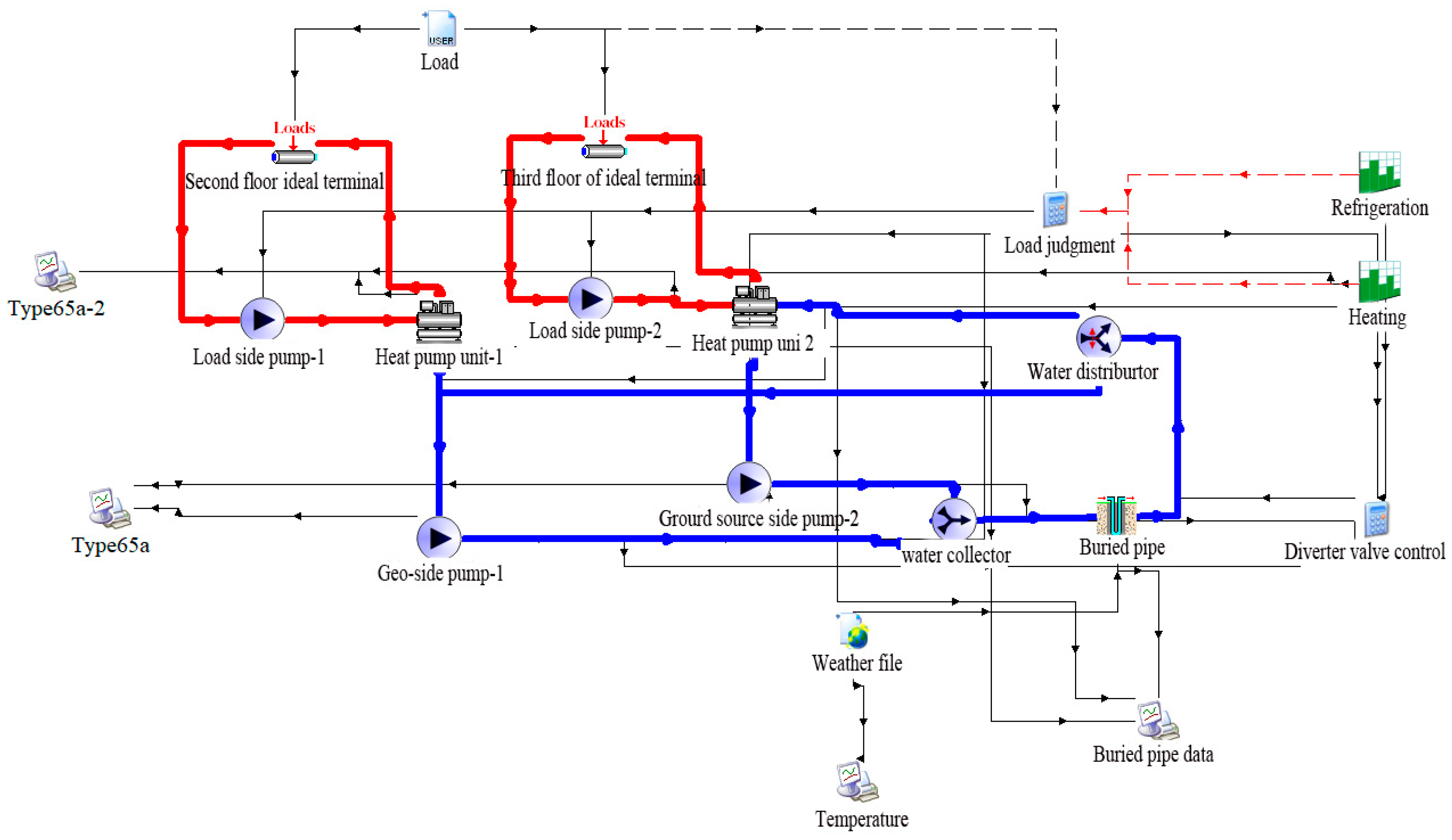
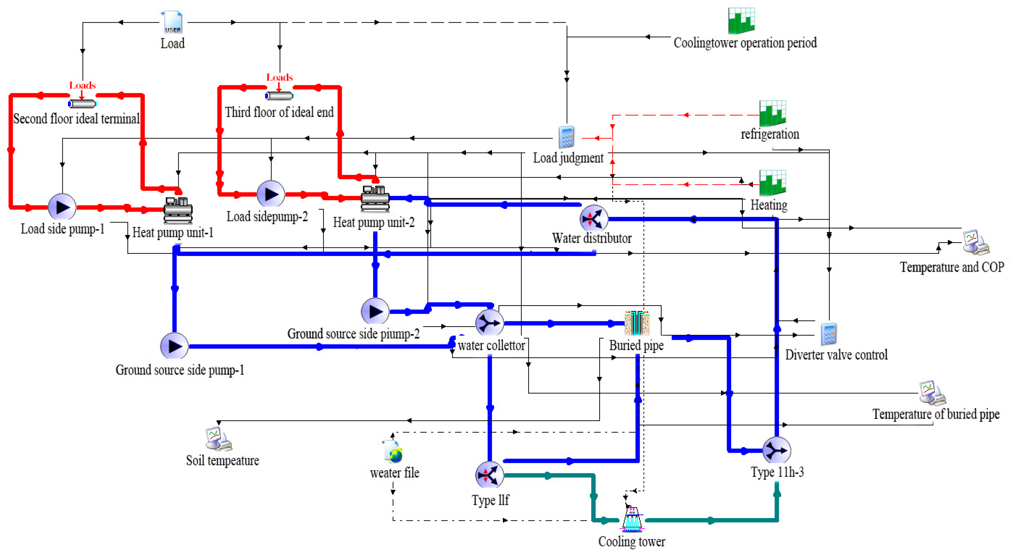
3.1. Build a Ground Source Heat Pump System Model

This paper used TRNSYS18 software to build a ground source heat pump model, which mainly uses modules such as heat pump unit module Type25 [21], underground heat exchange system module Type557 [22], and water pump module Type114. We used the Type9a module to call the hourly load of the project throughout the year and then import it into the model. The established model is shown in Figure 10.

The ground source heat pump system simulation model mainly controls the heat pump units, ground source-side and load-side water pumps, and water separators, and the control strategy is as follows:

① Control signal of heat pump unit

$$n1=Lt\left(fuhe2,0\right)$$

(1)

$$n2=Lt\left(fuhe3,0\right)$$

(2)

In the formula, n1 Heat pump unit 1 heating signal, connected to heat pump unit 1;

n2—Heat pump unit 2 heating signal, connected to heat pump unit 2;

fuhe2—Second floor terminal load, kJ/h;

fuhe3—Third floor terminal load, kJ/h;

Lt(a, b)—Return 1 if a is less than b and 0 otherwise.

② Control signals of ground source and load-side pumps

$$Pd1=Lt\left(fuhe2,-140400\ast 0.1\right)\ast zhire+Gt\left(fuhe2,121680\ast 0.1\right)\ast zhileng$$

(3)

$$Pd2=Lt\left(fuhe3,-140400\ast 0.1\right)\ast zhire+Gt\left(fuhe3,121680\ast 0.1\right)\ast zhileng$$

(4)

In the formula, zhire Heating signal;

zhileng—Cooling signal;

Pd1—Ground source water pump 1 indicates the signal of load-side water pump 1. When Pd1 = 1, the water pump runs;

Pd2—Ground source water pump 1 indicates the signal of load-side water pump 1. When Pd2 = 1, the water pump runs;

Gt(a, b)—Return 1 if a is greater than b and 0 otherwise.

③ Heating signal

Set the heating time to two specific ranges: from 0 to 1752 h and from 7608 to 8760 h, as illustrated in Figure 11.

④ Cooling signal

Set the cooling time to the range of 3216 to 6696 h, as depicted in Figure 12.

⑤ Water distributor signal

Set the output flow rate based on the flow ratio of the water pump at the ground source side.

$$M2=Pd\ast \left(m2\right)/\left(m1+m2\right)$$

(5)

In the formula, m1 flow through water pump 1 at the ground source;

m2—Flow through the ground source water pump 2;

Pd—When there is a cold or hot load, Pd = 1.

$$\mathrm{Pd}=(-1)\times \left(\mathrm{EQL}\right(\mathrm{Fuhe},0) - 1)$$

(6)

In the formula, Fuhe Cumulative value of layer 2 and layer 3 load, kj/h;

EQL(a, b)—Return 1 if a = b and 0 otherwise.

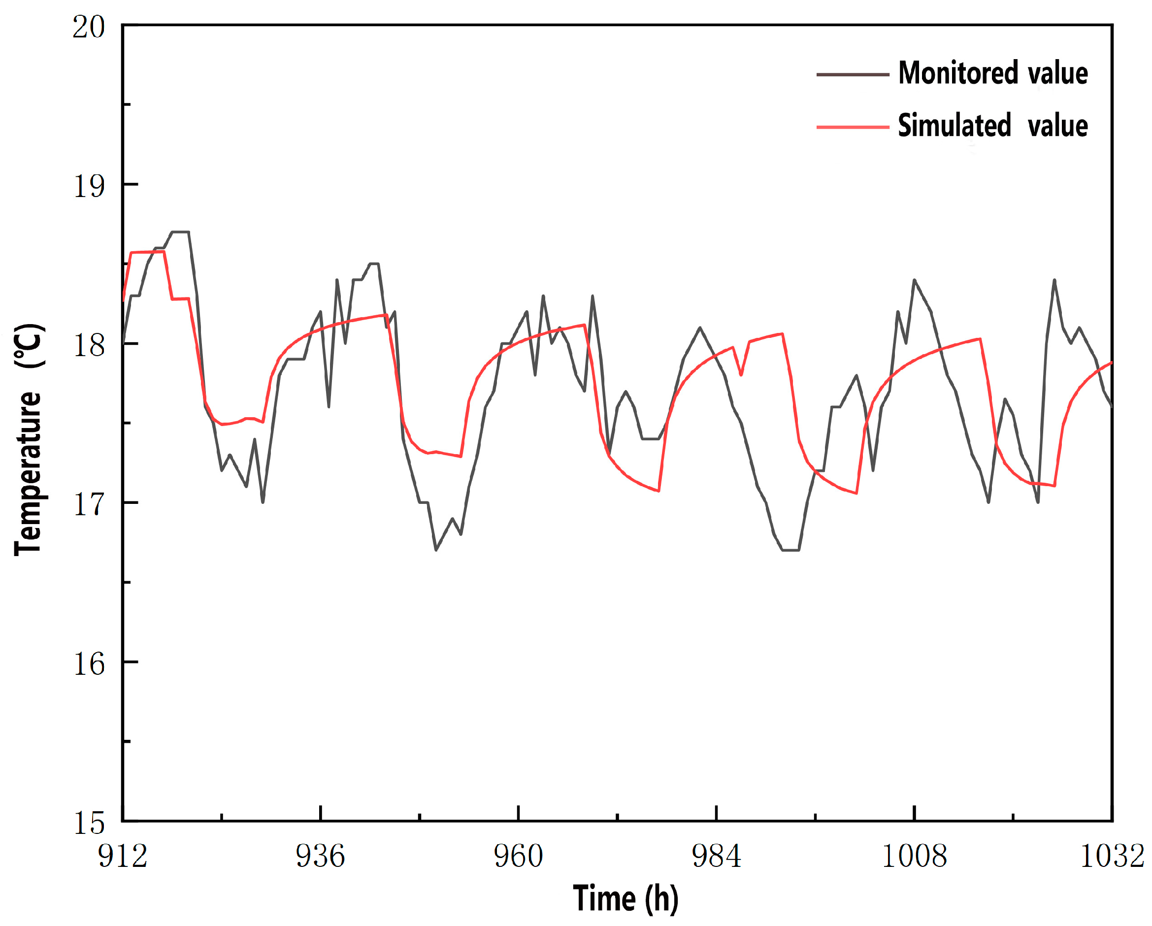
3.2. Model Verification

The monitoring data of the buried pipe inlet temperature are taken as the input element, and then the derived buried pipe outlet temperature is compared with the monitored one to verify the accuracy of the model [23]. Meanwhile, the model with maximum authenticity can be established by adjusting the soil thermal conductivity and other parameters [24]. We used the monitoring data from 0:00 on 8 February 2021 to 24:00 on 12 February 2021 for a period of 5 days as the basic data for winter operating condition validation for the validation of the simulation system.

Figure 13 shows the comparison between monitoring and simulation values of the outlet water temperature of buried pipes in winter. The average temperature of effluent from a buried pipe over 5 days was 17.71 °C, and the simulated value was 17.74 °C. The highest temperature of the outlet water from the buried pipe was measured at 918 h and 18.7 °C, and the highest temperature of the outlet water was simulated at 917 h and 18.58 °C.

The results show that the simulation value of the ground source heat pump system simulation model is in high agreement with the monitoring value, which can accurately reflect the change trend of a real ground source heat pump system and meet the use requirements. However, there are still some errors between the two, and the main reasons for the errors are as follows:

(1) The actual air conditioning time of the building is a certain lead time or delay, while in the simulation process, the terminal air conditioning equipment start and stop time is fixed, resulting in a deviation in the temperature curve.

(2) The simulation adopted the buried pipe heat exchanger module, the soil thermal conductivity is set to the average soil thermal conductivity, and the difference of thermal conductivity of different strata is not considered.

(3) Due to the quality of construction, in the process of burying the pipeline, the position of the temperature probe bound to the buried pipeline wall may move, and the PT100 temperature sensor has an irreducible measurement error.

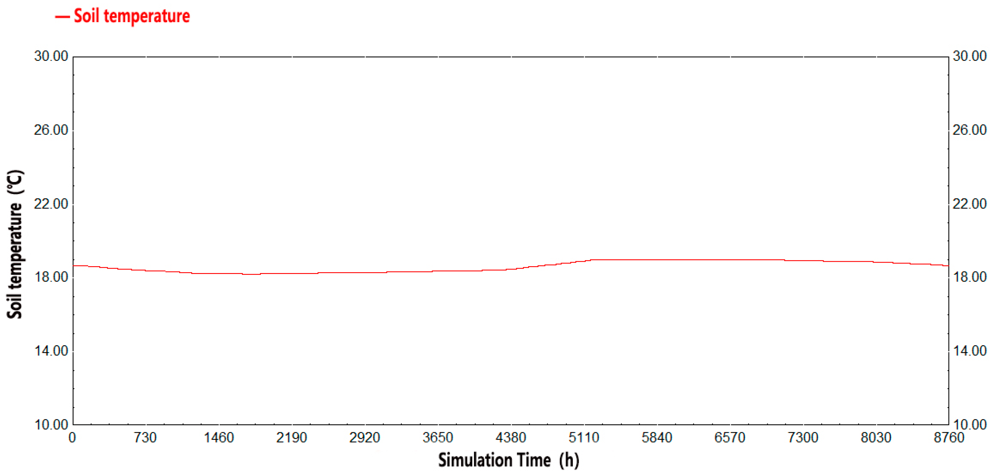
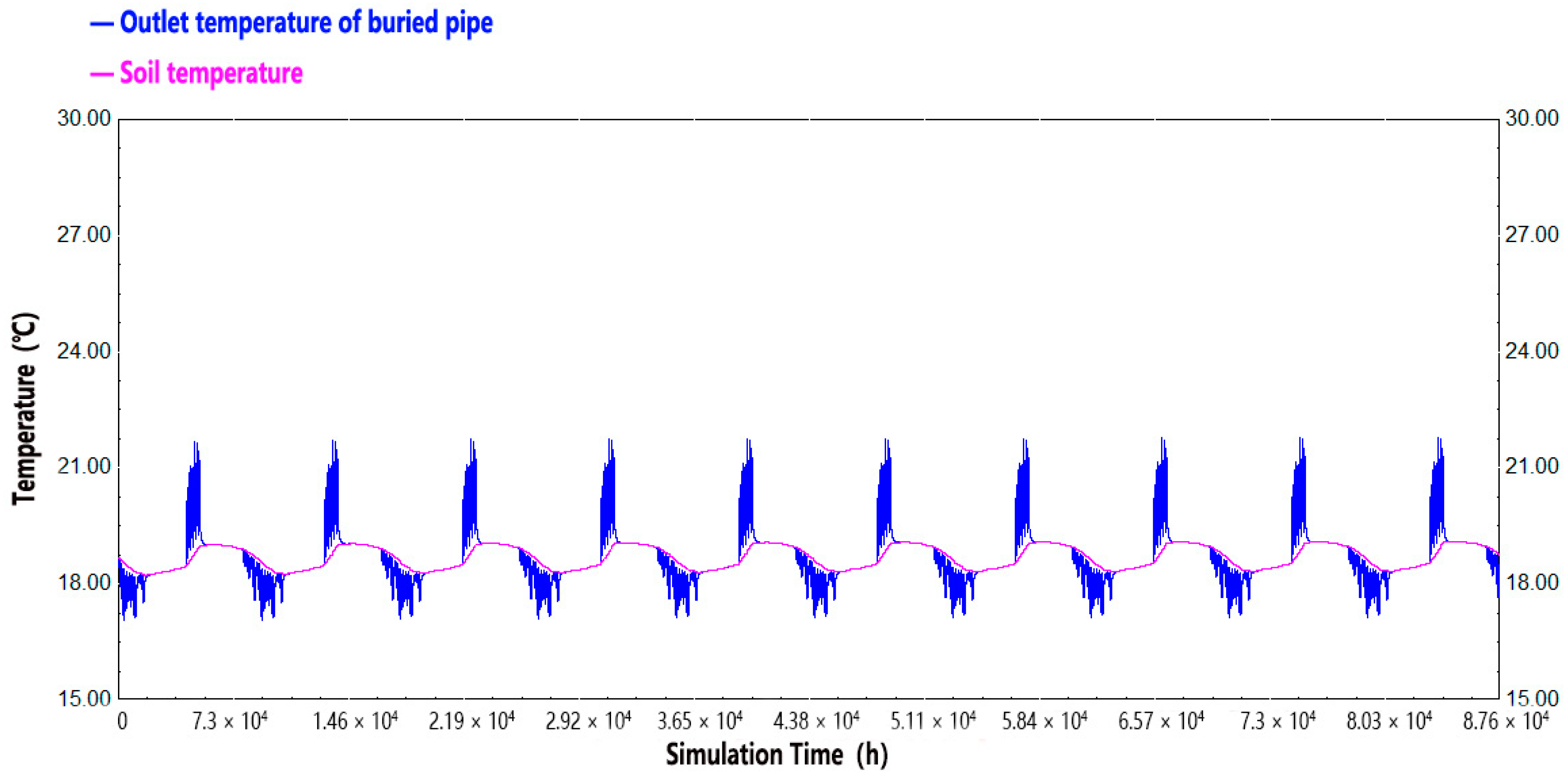
3.3. Long-Term Performance Analysis of Ground Source Heat Pump System

It can be seen from the simulation that the model of the ground source heat pump system can not only simulate the system energy supply under different operation strategies but also formulate the building operation strategies under different load conditions. However, in many cases, designers and operators want to understand the impact of system operation on soil temperature and system energy efficiency, so this paper will further analyze the long-term operation of GCHP systems. The original design parameters of the buried pipe are used as input parameters to adjust the buried pipe heat exchanger module in TRNSYS, and the model is simulated and operated.

3.3.1. The Simulation Model Was Run Continuously for 1 Year for Performance Analysis

Figure 14 shows the annual temperature change in the soil in the ground source heat pump system, indicating that the soil has increased by 0.46 °C, which is consistent with the annual increase in soil temperature obtained through linear heat source theory analysis (0.42 °C, with an error of 4.8%), further validating the accuracy of the ground source heat pump simulation model within the allowable range.

Figure 14 shows the soil temperature changes throughout the year. Figure 15 and Figure 16 show the annual return water temperature changes at the air conditioning side. It can be seen from the figures that the return water temperature in the winter is around 42 °C and the return water temperature in the summer is around 8 °C. The system operates well.

Figure 17 shows that the fluctuation of the inlet temperature of buried pipes in the summer is greater than that of the soil temperature, and the fluctuation of the inlet temperature of buried pipes in the winter is smaller than that of the soil temperature. This is because the cooling load required in the summer is greater than that required in the winter, leading to an increase in soil temperature and improving the performance of the winter soil source heat pump. The proper use of ground source heat pumps for heating in the winter can effectively transfer the imbalance of winter and summer loads to soil sources, and soil temperature can be well restored during the transition season with almost no heat accumulation problems. This can not only ensure the heating effect in winter and compensate for the decrease in cooling efficiency of soil source in summer but also transfer the heat accumulation problem caused by the imbalance of cold and hot loads in the ground source heat pump system.

From Figure 18, it can be seen that the performance coefficient of the heat pump unit in the summer is greater than that in the winter. When the cooling and heating load required by the building is small, the performance coefficient of the heat pump unit will also decrease. The average heating coefficient of performance in the winter is 3.79, and the average cooling coefficient of performance in the summer is 6.63.

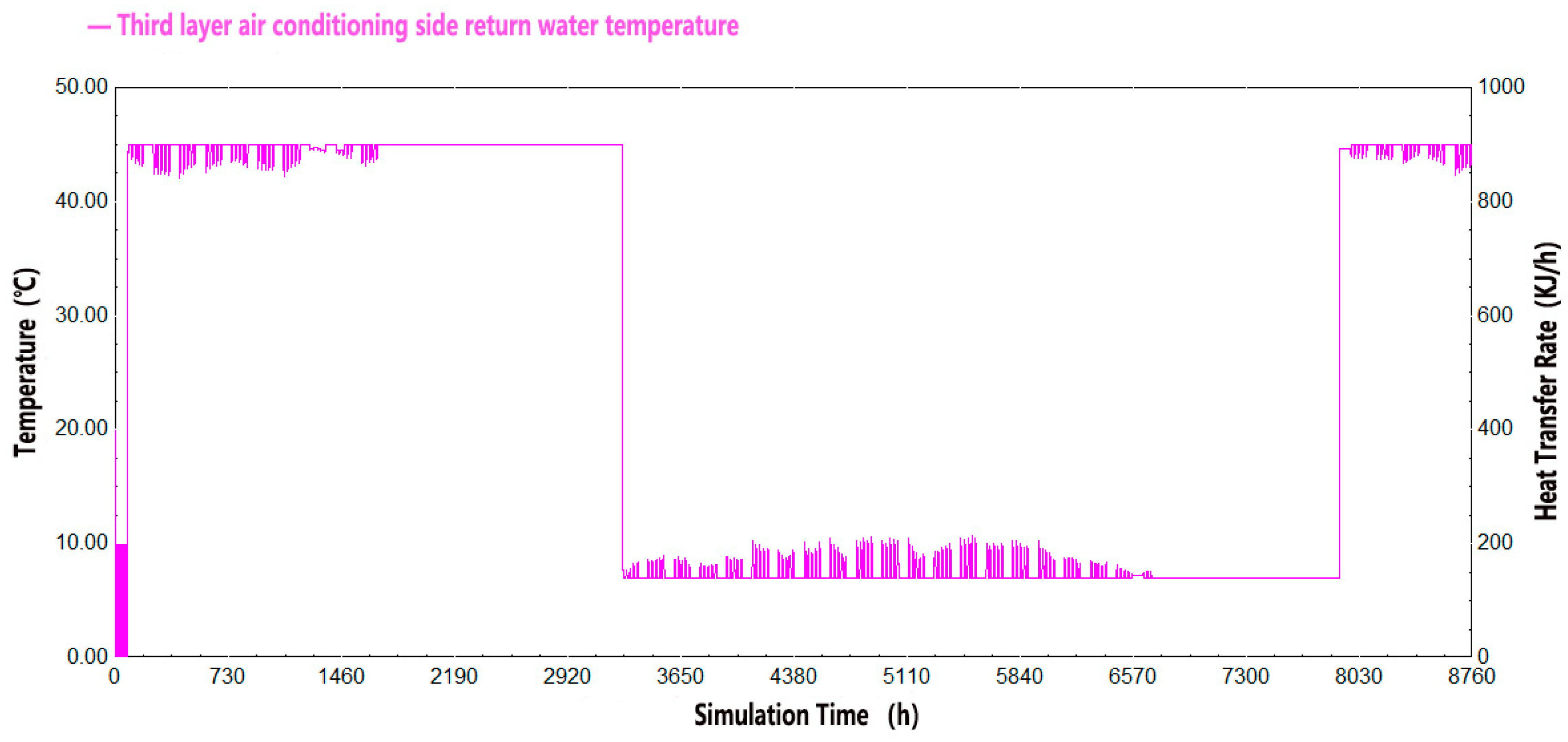
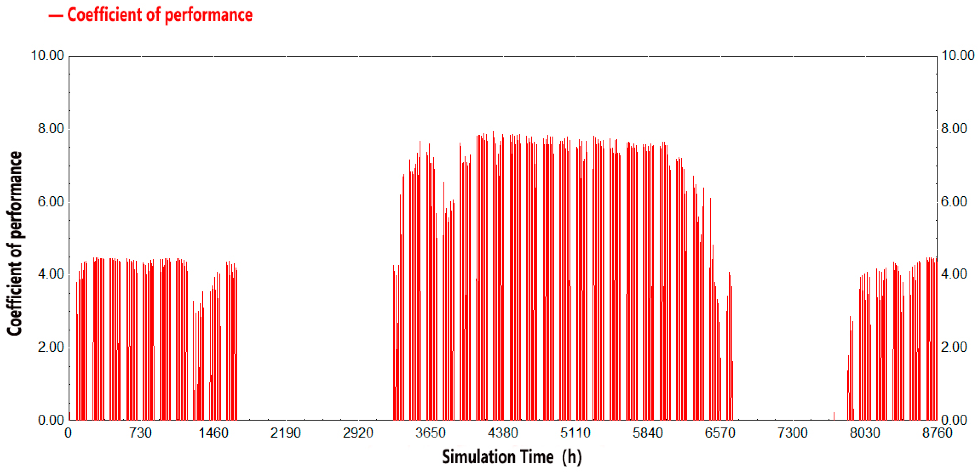
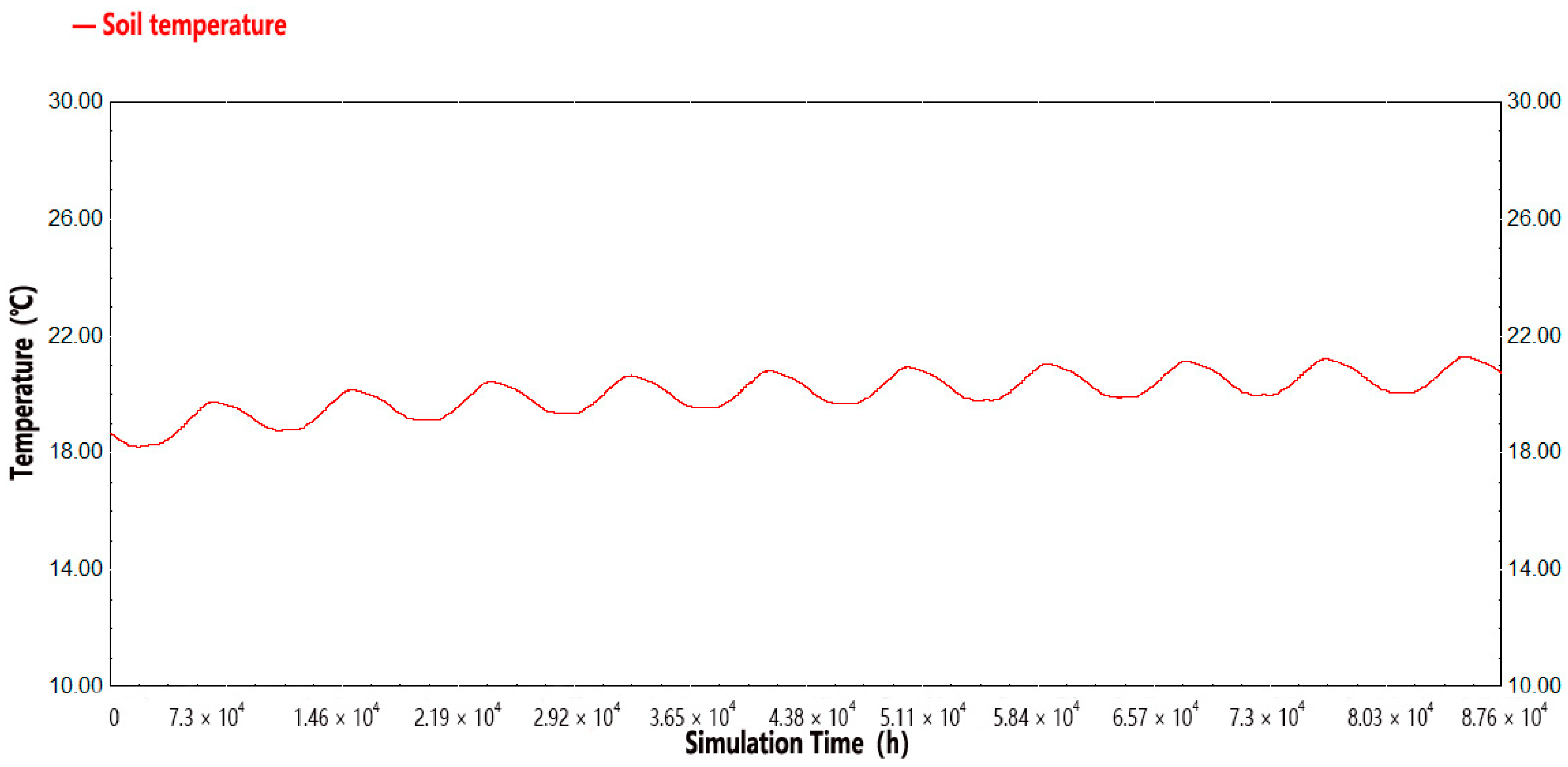
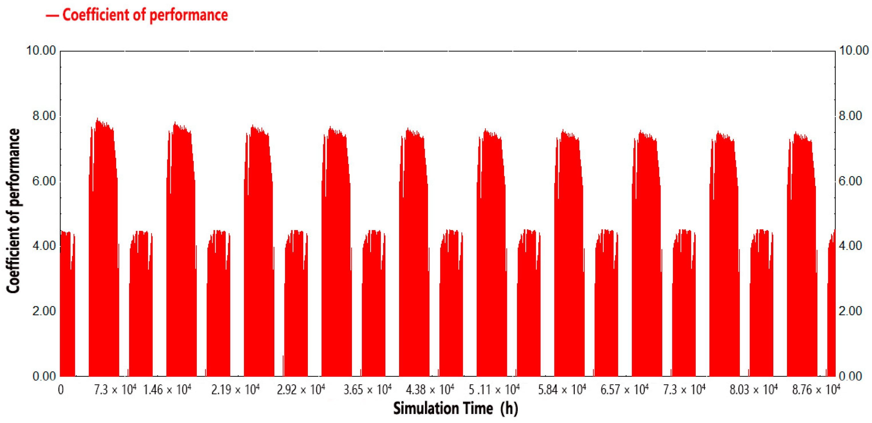
3.3.2. The Simulation Model Was Run Continuously for 10 Years for Performance Analysis

The simulation model of the ground source heat pump was simulated for 10 years. As shown in Figure 19, it can be seen that due to the cooling load required by the system being greater than the heating load, the average soil temperature shows an increasing trend year on year. And the rate of increase is relatively fast in the first few years of operation as well as by the end of the 10th year. The average soil temperature reaches 20.74 °C, with a cumulative increase of 2.05 °C, indicating that thermal accumulation occurred. The average soil temperature changes with the changes in the heat exchange environment of buried pipes, and any significant changes in the soil temperature during system operation will affect the stability of the system’s operation.

Figure 20 shows the performance coefficient variation in the heat pump unit after 10 years of operation. It can be seen from Figure 20 that the winter performance coefficient of the heat pump unit remains almost unchanged. From Figure 21, it can be seen that the performance coefficient of the heat pump unit gradually decreases during long-term operation in the summer. The analysis is that the increase in soil temperature in the buried pipe area leads to a decrease in the efficiency of the buried pipe heat exchanger, resulting in a decrease in the cooling capacity of the heat pump unit in summer. Under the same electricity consumption, the cooling performance coefficient of the heat pump unit decreases.

4. Analysis of Cooling Tower Auxiliary Ground Source Heat Pump System and Control Strategy

4.1. Cooling Tower Module Settings

Cooling tower selection is a Type 51b module. When the cooling tower is in operation, heat transfer occurs between the sprayed water and the air due to the temperature difference. Driven by the airflow produced by the cooling tower fan, the hot air exchanged with the water is expelled, achieving the cooling effect [25]. Considering constant parameters of ground source heat pump system equipment, we designed calculations for only the cooling tower equipment. First, the cooling water quantity was designed. Formula (7) is the design calculation of the cooling water quantity of the cooling tower, which is calculated on the premise of the maximum bearing cooling load.

$$m={\displaystyle \frac{3.6kQ}{C(t_1-t_2)}}$$

(7)

In the formula, m—Cooling tower cooling water, m³/h;

Q—Cooling capacity of heat pump unit, kW;

k—The heat coefficient of the heat pump unit during refrigeration is 1.2 [26];

c—The specific heat capacity of water is 4.19 kJ/(kg·°C) [26];

t₁—Inlet water temperature of the cooling tower, °C; the cooling tower inlet temperature here is set to 37 °C [26];

t₂—Outlet water temperature of the cooling tower, °C; The cooling tower outlet temperature here is set to 32 °C [26].

According to the formula, the volume of the cooling tower is 13.94 m³/h, so the GLT-15L counter-current circular tower is selected, the flow rate is 15.62 m³/h, the motor power is 0.37 kW, the net weight is 80 kg, and the operating weight is 320 kg.

4.2. Establishment of the Cooling Tower Auxiliary Ground Source Heat Pump System Model

A cooling tower auxiliary ground source heat pump system model is constructed based on the established ground source heat pump simulation model, as illustrated in Figure 22.

The cooling tower auxiliary ground source heat pump system model mainly controls the cooling tower modules, while other module control conditions are consistent with the ground source heat pump simulation model, and the cooling tower control strategy is as follows:

$$cooling2=Gt\left(fuhe2,0\right)$$

(8)

$$cooling3=Gt\left(fuhe3,0\right)$$

(9)

$$\mathit{\text{lqt\_kz}}=Max\left(cooling2, cooling3\right)\ast Max\left(pd2,pd3\right)\ast lqt$$

(10)

In the formula, the following apply: cooling2—If the layer 2 load is greater than 0, it is 1; otherwise, it is 0;

cooling3—When the three-layer load is greater than 0, it is 1, otherwise it is 0;

Max(a, b)—Take the maximum of a and b;

lqt—Cooling tower running time;

lqt_kz—Cooling tower control signal;

4.3. Optimization Analysis of Cooling Tower Auxiliary Ground Source Heat Pump System

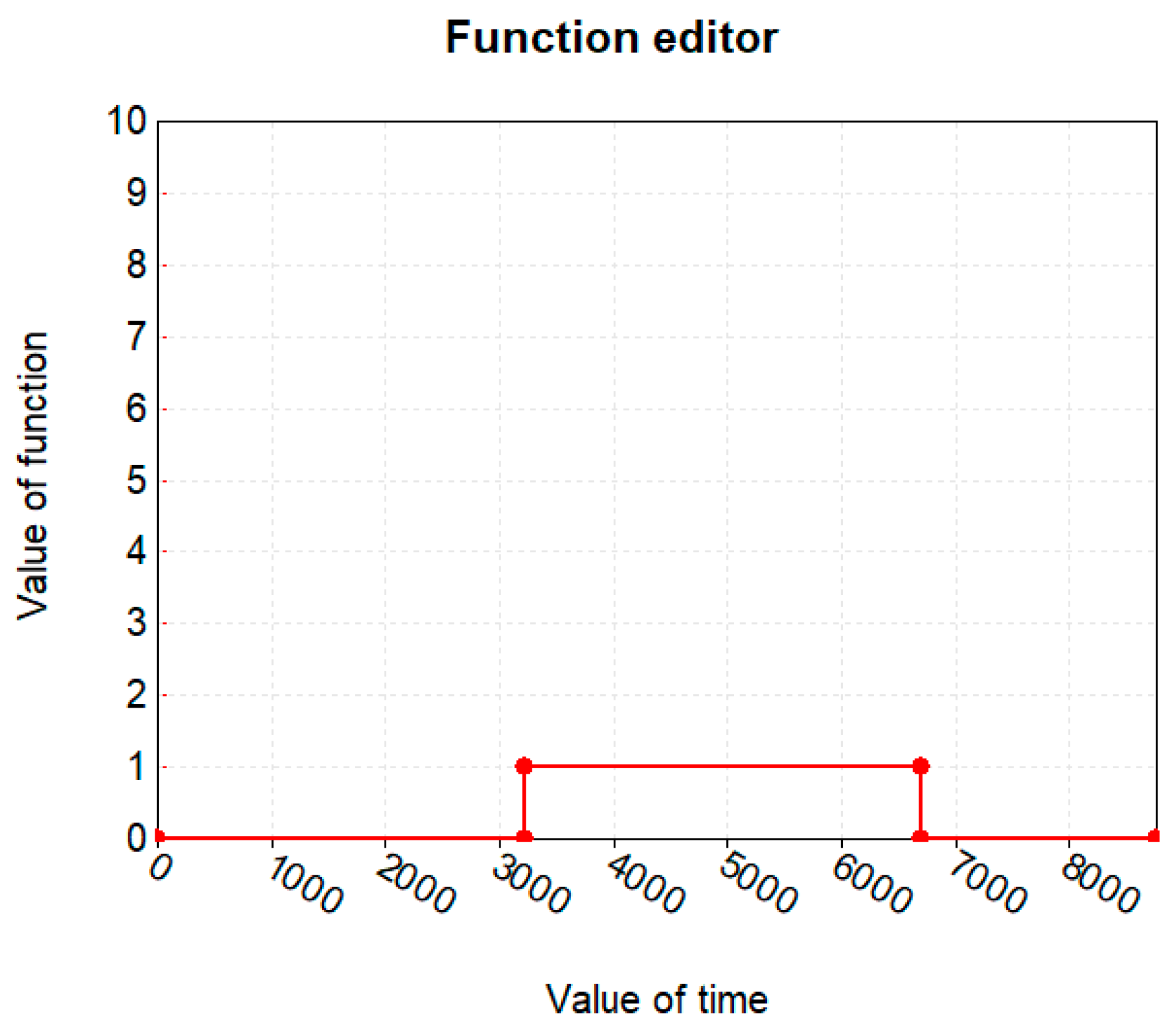
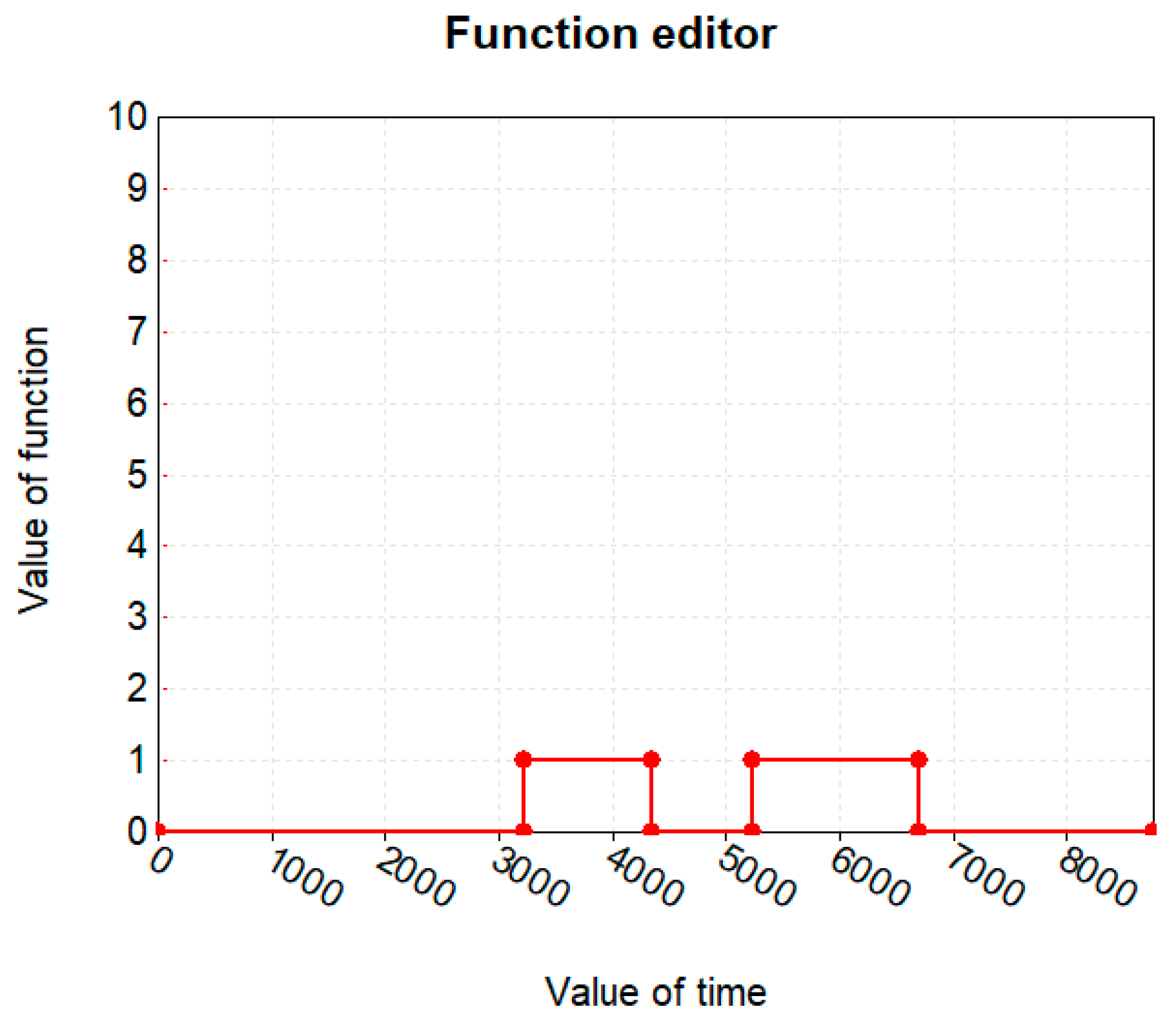
4.3.1. Control Strategy Analysis

The whole refrigeration season is roughly divided into three periods: the early, middle and late stages of the refrigeration season. The outdoor air wet bulb temperature is a key measure that indicates the temperature of air when it is saturated with moisture. It is determined using a thermometer with a wetted bulb, which shows the cooling effect of evaporation. Figure 23 is a schematic diagram of the outdoor air wet bulb temperature. It can be seen that the outdoor wet bulb temperature is lower in the early and late stages of the cooling season than in the middle stage. The outdoor wet bulb temperature affects the efficiency of the cooling tower. The low outdoor wet bulb temperature is beneficial to cooling tower refrigeration, so the efficiency of the cooling tower in the early and late refrigeration season is higher than that in the middle stage. For this reason, the operating time of the cooling tower is controlled.

By observing the temperature rise of soil after one year, the operation time of the cooling tower is continuously adjusted. When the soil temperature is the same as the initial soil temperature after one year, the start–stop time of the cooling tower is the optimal operation time of the cooling tower. The ideal operational hours for the cooling tower are 3216–4344 h and 5424–6696 h, as illustrated in Figure 24.

4.3.2. Simulation Results

The cooling tower auxiliary ground source heat pump system was simulated for one year. From Figure 25, it can be seen that the soil temperature of the optimized cooling tower auxiliary ground source heat pump system remains consistent with the initial temperature after one year, and there is no heat accumulation.

4.4. Comparison of GCHP and HGSHP Systems

The changes in the outlet water temperature and soil temperature of buried pipes with GCHP and HGSHP operating for ten years are shown in Figure 26 and Figure 27.

As can be seen from Figure 27, for the HGSHP system, the soil temperature and outlet temperature of the buried pipes are relatively stable over long-term operation. Basically, by controlling the running time of the cooling tower, the soil temperature can be restored to the initial temperature almost every year. In addition, the outlet temperature of the buried pipes is almost constant over ten years of operation. These results show that it is feasible to use the HGSHP system for heating and cooling.

5. Conclusions

This study focused on optimizing a ground source heat pump (GSHP) system using the TRNSYS simulation tool specifically for regions with hot summers and cold winters. The research set out to achieve several key objectives, including the development of a precise building load calculation model, the establishment of a comprehensive GSHP system model, long-term performance analysis, and the exploration of the benefits of integrating a cooling tower as an auxiliary system. The results of this research can be summarized as follows:

(1) The dynamic load simulation results indicate that in the studied building, there is a significant disparity between cooling and heating demands, with a cumulative cooling load of 30,029 kWh for both the second and third floors compared to a cumulative heating load of 15,339 kWh. This leads to a ratio of cumulative cooling to heating load of 1.96:1, reflecting the predominance of cooling requirements over heating in this hot summer and cold winter climate. Consequently, the heating demand during winter is considerably lower than the cooling demand in summer, emphasizing the need for a system designed primarily to address cooling loads.

(2) The simulation of the GSHP system over one year showed a soil temperature increase of 0.46 °C. After ten years of operation, the soil temperature rose by a more significant 2.05 °C. The heating performance coefficient largely remained stable during the winter months; however, the cooling performance coefficient exhibited a gradual decline during the summer. This highlights the importance of monitoring soil temperature and its implications for the long-term performance of the GSHP system.

(3) The study established a cooling tower-assisted GSHP system, evaluating the optimal operation times for the cooling tower, which ranged from 3216 to 4344 h and 5424 to 6696 h. During a ten-year operational period, this system maintained stable soil temperatures and consistent outlet temperatures from the buried pipes, effectively mitigating thermal imbalances. The cooling tower’s integration serves as an essential auxiliary measure to enhance the performance of the GSHP particularly during peak cooling periods in the summer.

(4) The comparative analysis demonstrated that the cooling tower-assisted GSHP system outperforms the standalone GSHP system in terms of long-term operational efficiency and sustainability. The hybrid system exhibited a more balanced thermal load distribution and improved heat exchange efficiency over extended periods. This suggests that incorporating auxiliary components like cooling towers is a feasible and effective strategy for heating and cooling in climates characterized by hot summers and cold winters.

References

1. Yuan, J.; Kang, J.; Yu, C.; Hu, Z. Energy conservation and emissions reduction in China—Progress and prospective. Renew. Sust. Energ. Rev. 2011, 15, 4334–4347. [Google Scholar] [CrossRef]
2. Zhang, G. Energy conservation, emission reduction and environmental protection under the new circumstances. Creat. Living 2022, 11, 151–153. [Google Scholar]
3. Yang, W. Discussion on energy conservation, emission reduction and environmental protection under the new situation. Resour. Econ. Environ. Prot. 2022, 9–12. [Google Scholar]
4. Neamţu, O.M.; Roşca, M.G.; Bendea, C.C. Monitoring and data acquisition system for a geothermal heat pump. In Proceedings of the 2014 International Symposium on Fundamentals of Electrical Engineering (ISFEE), Bucharest, Romania, 28–29 November 2014; IEEE: Piscataway, NJ, USA, 2014. [Google Scholar]
5. Jin, G.; Chen, Z.; Guo, S.; Hao, N. Feasibility study of solar energy-ground source heat pump system heating in Inner Mongolia region. Acta Energiae Solaris Sin. 2021, 42, 334–341. [Google Scholar]
6. Hu, J. Analysis of Heat Balance in Ground Source Heat Pump System and Its Application in Large Scale Public Buildings. Chin. J. Refrig. Technol. 2015, 35, 63–67. [Google Scholar]
7. Ma, L.; Ren, T.; Zhen, X.; Zhang, J. Experimental Analysis of effect of inlet and outlet water temperature on performance of heat pump unit with large temperature difference bathing wastewater source. J. Civ. Environ. Eng. 2019, 41, 170–178. [Google Scholar]
8. Liu, Z.; Li, Y.; Xu, W.; Yin, H.; Gao, J.; Jin, G.; Lun, L.; Jin, G. Performance and feasibility study of hybrid ground source heat pump system assisted with cooling tower for one office building based on one Shanghai case. Energy 2019, 173, 28–37. [Google Scholar] [CrossRef]
9. Qiu, G.; Li, K.; Cai, W.; Yu, S. Optimization of an integrated system including a photovoltaic/thermal system and a ground source heat pump system for building energy supply in cold areas. Appl. Energy 2023, 349, 121698. [Google Scholar] [CrossRef]
10. Cui, W.; Zhou, S.; Liu, X. Optimization of Design and Operation Parameters for Hybrid Ground-Source Heat Pump Assisted with Coo. Energy Build. 2015, 99, 253–262. [Google Scholar] [CrossRef]
11. Xie, Y.; Hu, P.; Peng, D.; Zhu, N.; Lei, F. Development of a group control strategy based on multi-step load forecasting and its application in hybrid ground source heat pump. Energy 2023, 273, 127196. [Google Scholar] [CrossRef]
12. Yang, J.; Xu, L.; Hu, P.; Zhu, N.; Chen, X. Study on Intermittent Operation Strategies of a Hybrid Ground-Source Heat Pump System with Double-Co. Energy Build. 2014, 76, 506–512. [Google Scholar] [CrossRef]
13. Deng, F.; Li, W.; Pei, P.; Wang, L.; Ren, Y. Study on design and calculation method of borehole heat exchangers based on seasonal patterns of groundwater. Renew. Energy 2024, 220, 119711. [Google Scholar] [CrossRef]
14. Chen, D. Research on Operational Characteristics of Hybrid Ground Source Heat pump with the Auxiliary Cooling Tower. Ph.D. Thesis, Yangzhou University, Yangzhou, China, 2016. [Google Scholar]
15. Fan, Q.; Yuan, L.; Zhao, C.; Tian, R. Study on optimization and time effect of ground-source heat pump system in Nanjing. Hydrogeol. Eng. Geol. 2024, 51, 233–242. [Google Scholar]
16. Wang, C. Ground Source Heat Pump Based on TRNSYS in a Building in Beijing Study on System Operation Optimization. Ph.D. Thesis, Hebei University of Architecture, Zhangjiakou, China, 2022. [Google Scholar]
17. Seung-Hoon, P.; Eui-Jong, K. Achieving a mitigation of ground thermal imbalance and size-reduction of borehole heat exchangers by connecting a hybrid heat source in series. Appl. Therm. Eng. 2024, 243, 122593. [Google Scholar]
18. Chen, L.; Zhang, X.; Zhang, Y. Performance analysis of a ground source heat pump system integrated with a cooling tower. Energy Build. 2020, 212, 109749. [Google Scholar]
19. Michael, W. GenOpt(R), Generic Optimization Program, User Manual, Version 2.0.0; Lawrence Berkeley National Laboratory: Berkeley, CA, USA, 2003.
20. Xiang, Y. Research on the Performance of Heat Transfer and Heat Pump System of Heat Source Tower. Ph.D. Thesis, Chongqing University, Chongqing, China, 2021. [Google Scholar]
21. Yang, S. Simulation Study of Variable Flow System of Ground Source Heat Pump Based on TRNSYS Buried Pipe. Ph.D. Thesis, Shandong Jianzhu University, Jinan, China, 2016. [Google Scholar]
22. Hellström, G. Ground heat storage: Thermal Analyses of Duct Storage Systems. Master’s Thesis, Lund University, Lund, Sweden, 1991. [Google Scholar]
23. Huang, X. Simulation and Optimization of Ground Source Heat Pump System Based on TRNSYS. Ph.D. Thesis, Suzhou University of Science and Technology, Suzhou, China, 2019. [Google Scholar]
24. Thornton, J.W.; McDowell, T.P.; Shonder, J.; Hughes, P.; Pahud, D.; Hellström, G. Residential vertical geothermal heat pump system models calibration to data. ASHRAE Trans. 1997, 103, 660–674. [Google Scholar]
25. Tang, P. Study on Optimization of Construction Scheme for High-Rising Building Based on New Engineering Concept. Ph.D. Thesis, Central South University, Changsha, China, 2013. [Google Scholar]
26. Baker, R.C. Cooling Tower Performance: Design Calculations and Parameters. ASHRAE J. 2015, 57, 34–42. [Google Scholar]
Figure 1. Layout plan of ground temperature monitoring hole and buried pipe monitoring hole.
Buildings 14 02764 g001
Figure 2. Full-year dynamic load calculation model.
Buildings 14 02764 g002
Figure 3. Annual and hourly outdoor dry bulb temperature in the project area.
Buildings 14 02764 g003
Figure 4. Average outdoor dry ball temperature in project area.
Buildings 14 02764 g004
Figure 5. The 3D physical model of the building.
Buildings 14 02764 g005
Figure 6. Utilization rate of (a) office staff, (b) office lighting, and (c) office equipment.
Buildings 14 02764 g006
Figure 7. Schematic diagram of the building load parameter setting interface.
Buildings 14 02764 g007
Figure 8. Annual and time-dependent load of the second floor of a building.
Buildings 14 02764 g008
Figure 9. Annual hourly load on the third floor of the building.
Buildings 14 02764 g009
Figure 10. Simulation model of ground source heat pump system.
Buildings 14 02764 g010
Figure 11. Heating time.
Buildings 14 02764 g011
Figure 12. Cooling time.
Buildings 14 02764 g012
Figure 13. Monitoring value and simulated value of buried pipe effluent temperature in winter.
Buildings 14 02764 g013
Figure 14. Variation in soil temperature throughout the year.
Buildings 14 02764 g014
Figure 15. Annual return water temperature of the air conditioner on the second floor.
Buildings 14 02764 g015
Figure 16. Annual return water temperature at the third floor air conditioner side.
Buildings 14 02764 g016
Figure 17. Annual buried pipe inlet temperature and soil temperature.
Buildings 14 02764 g017
Figure 18. Performance coefficient changes of heat pump units throughout the year.
Buildings 14 02764 g018
Figure 19. Soil average temperature change curve of ground source heat pump system for 10 years.
Buildings 14 02764 g019
Figure 20. Change in performance coefficient of the heat pump unit after 10 years of operation of the ground source heat pump system.
Buildings 14 02764 g020
Figure 21. EER change in the heat pump unit of the ground source heat pump system after 10 years of operation.
Buildings 14 02764 g021
Figure 22. Simulation model of cooling tower auxiliary ground source heat pump system.
Buildings 14 02764 g022
Figure 23. Outdoor wet bulb temperature.
Buildings 14 02764 g023
Figure 24. Optimal time control of cooling tower.
Buildings 14 02764 g024
Figure 25. Annual soil temperature changes after optimization.
Buildings 14 02764 g025
Figure 26. Changes of outlet water temperature and soil temperature over ten years of GCHP operation.
Buildings 14 02764 g026
Figure 27. Changes of outlet water temperature and soil temperature during ten years of HGSHP operation.
Buildings 14 02764 g027