

Evaluation and Optimization of Traditional Mountain Village Spatial Environment Performance Using Genetic and XGBoost Algorithms in the Early Design Stage—A Case Study in the Cold Regions of China


Abstract
:1. Introduction
2. Methods
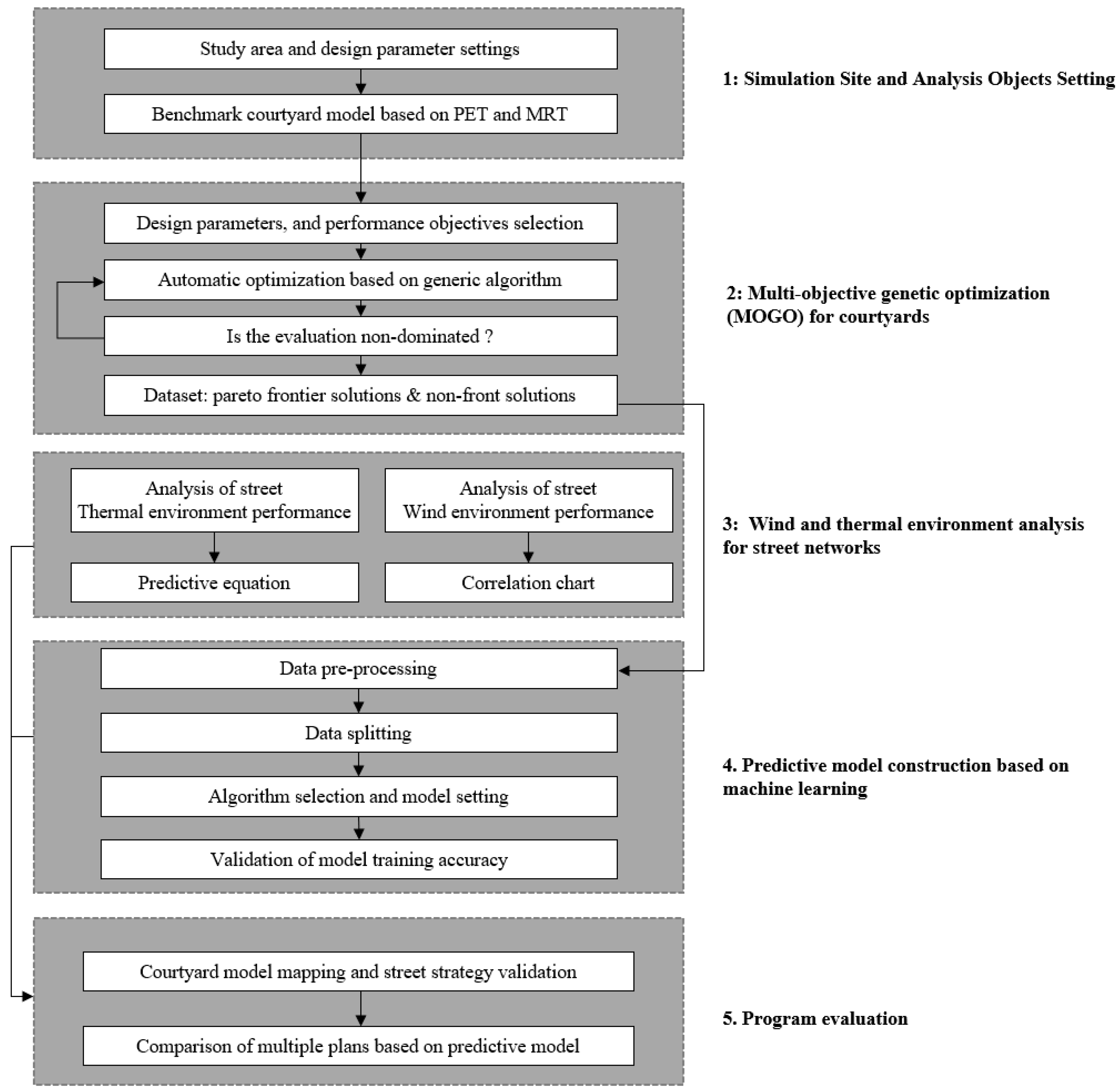
2.1. Overview Workflow
- (1)
- Simulation site and analysis objects settings: A benchmark courtyard model was selected by simulating and ranking PET and MRT values across various courtyard types using Honeybee 0.0.66 software.
- (2)
- Multi-objective genetic optimization (MOGO) for courtyards. The benchmark courtyard model underwent refinement through MOGO using the Wallacei_X plugin, generating a dataset for subsequent machine learning.
- (3)
- Wind and thermal environment analysis for street networks. Performance simulations of the wind environment within street networks were conducted, and their correlation with spatial elements was analyzed. Additionally, thermal environment simulations at different analysis radii were performed to examine the relationship between comfort and spatial elements, leading to the establishment of stepwise regression predictive equations.
- (4)
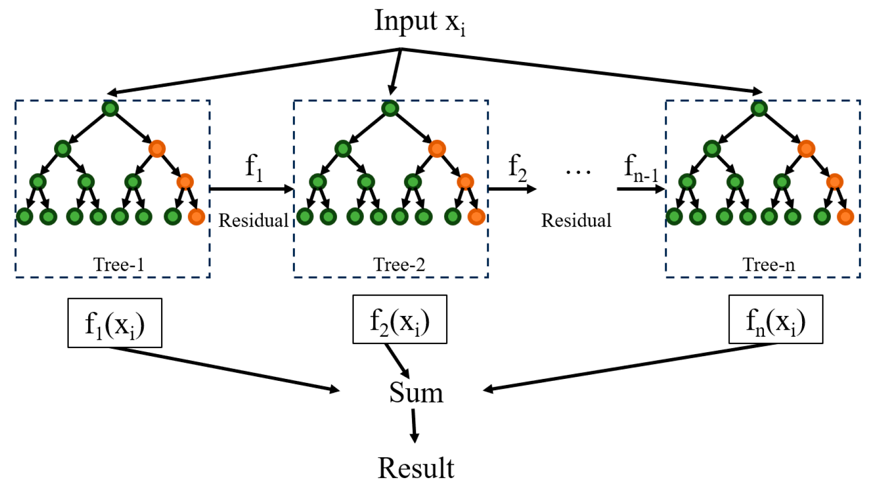
- Predictive model construction based on machine learning: The courtyard dataset was processed in Scikit-learn 1.3 and trained using the XGBoost algorithm to create a predictive model for courtyard performance.
- (5)
- Program evaluation: Various design plans were proposed based on different target objectives. The data parameters of each solution were input into the algorithm model for performance evaluation, allowing for the selection of the most optimal design.
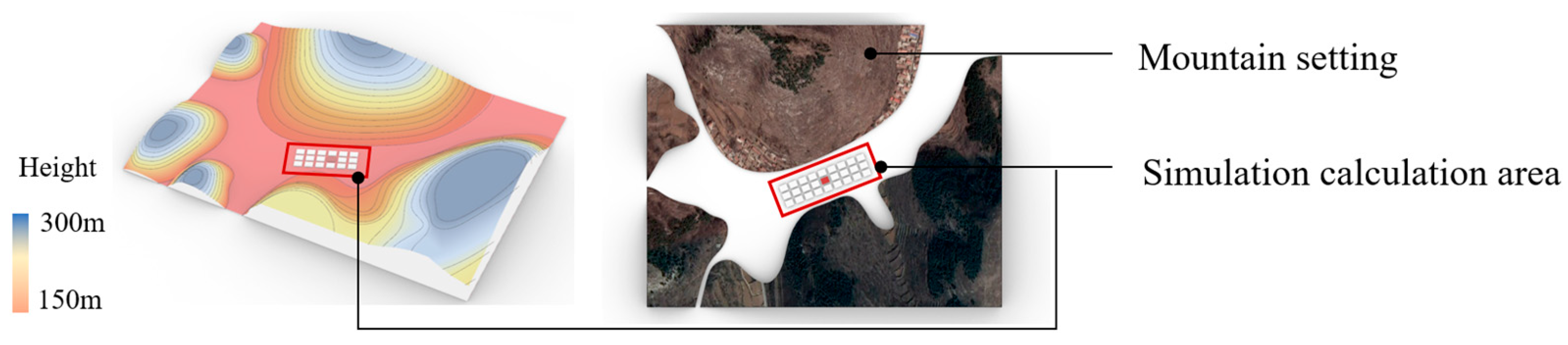
2.2. Simulation Site and Analysis Objects Settings
2.2.1. Site Selection for This Study
- (1)
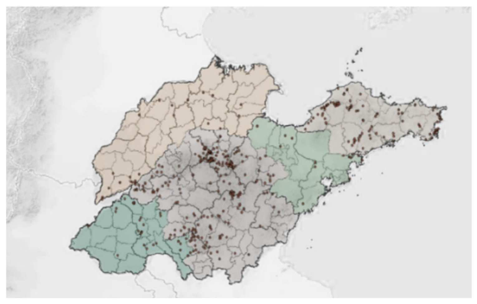
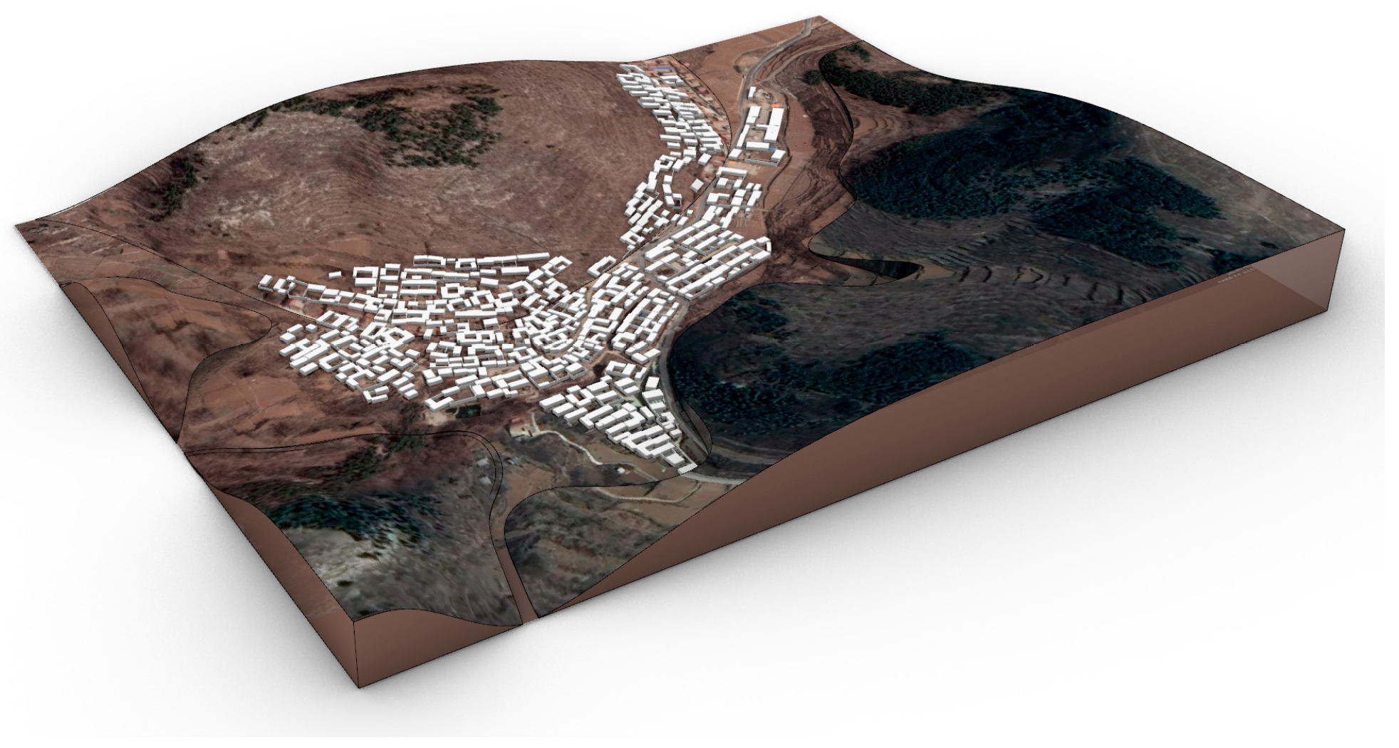
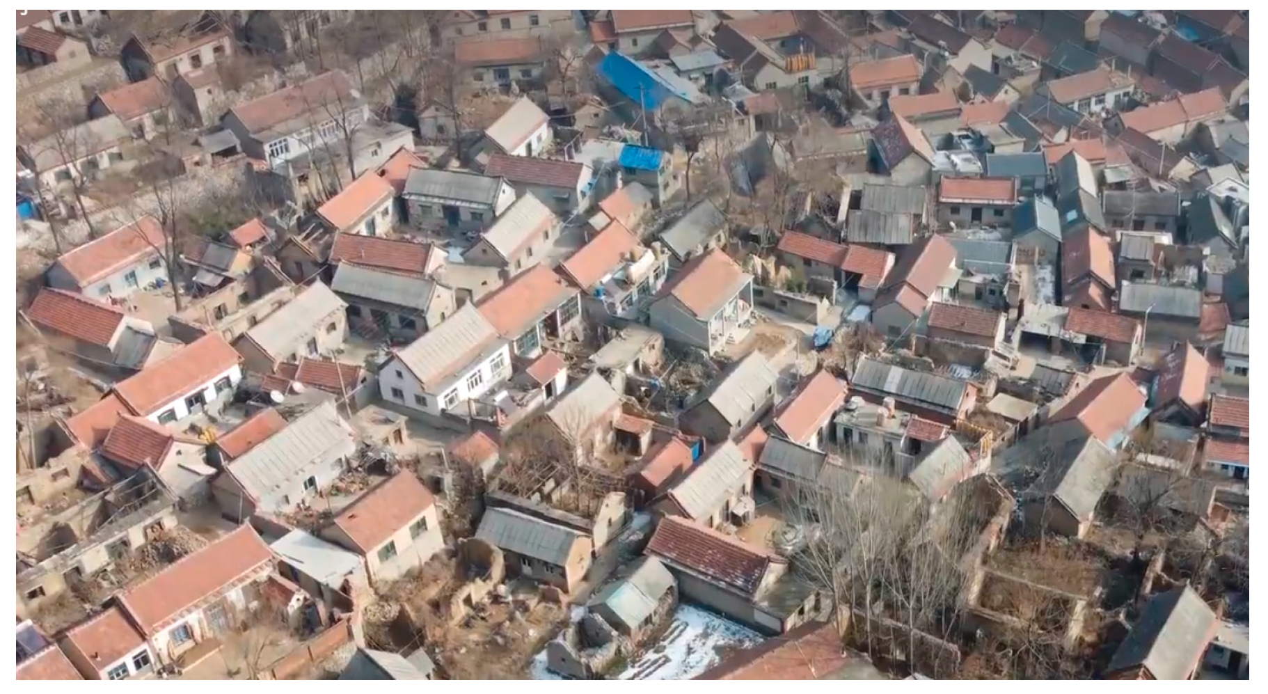
- Mountainous Location: Village A is situated in a mountainous area. According to ArcGIS 10.8 statistical analysis of village distribution in Shandong Province, most traditional villages are in mountainous regions. Using a cluster statistical analysis method, this study overlayed the distribution of 519 villages in Shandong with a 30-m resolution digital elevation model (DEM) of the province, resulting in a topographic map of village distribution (Figure 2). The statistical results reveal that approximately 57% of the villages are situated at elevations exceeding 100 m (Table 1), primarily concentrated in the central mountainous region of Shandong.
- (2)
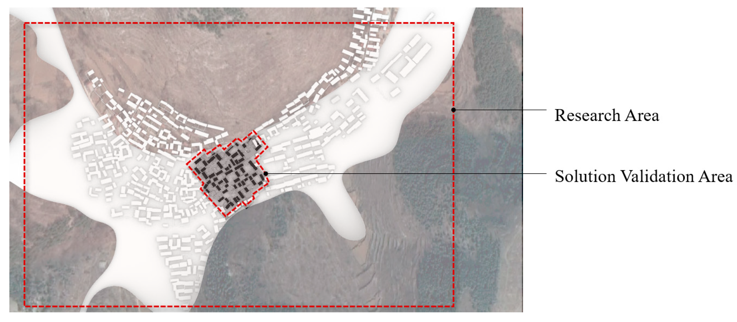
- Distance from Urban Areas: Village A is far from urban centers. To ensure the independence of the study subject and minimize the influence of urban heat island effects, the selected site is over 40 km away from several city centers (Figure 3). The mountainous terrain further reduces the impact of urban heat island effects.
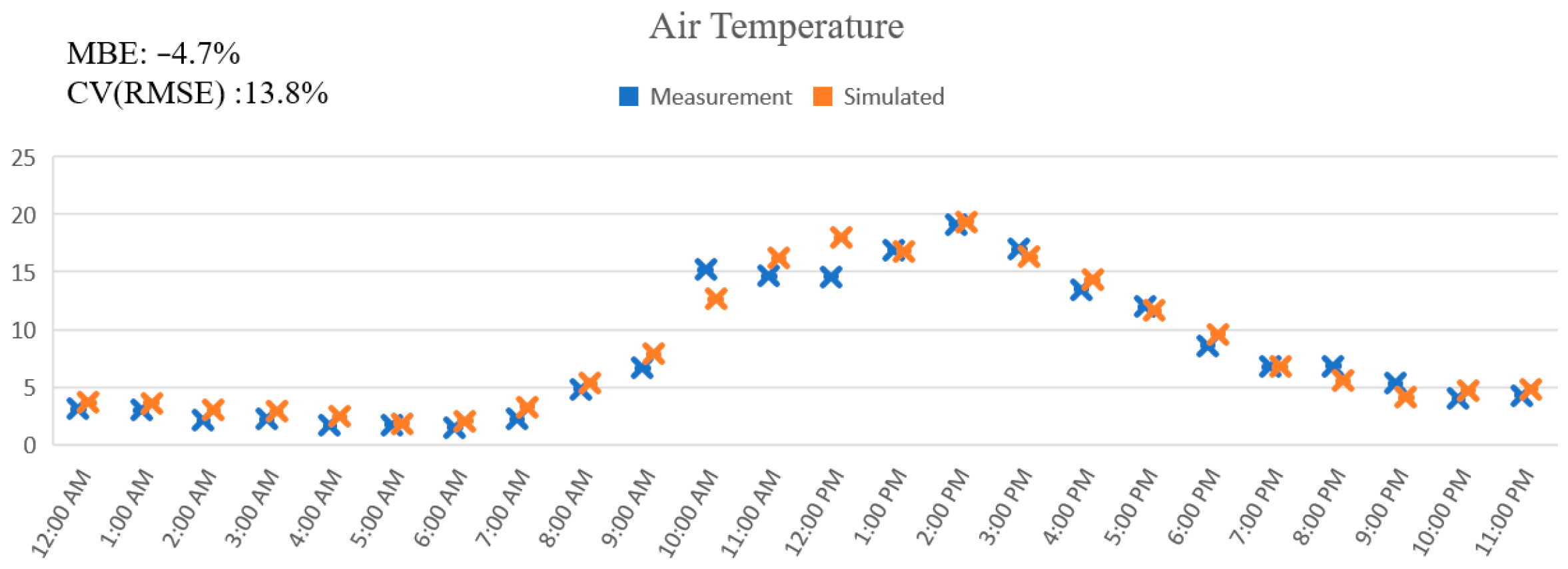
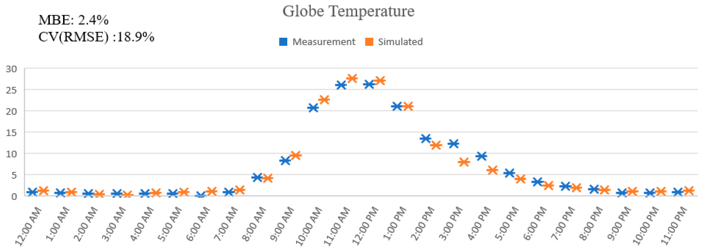
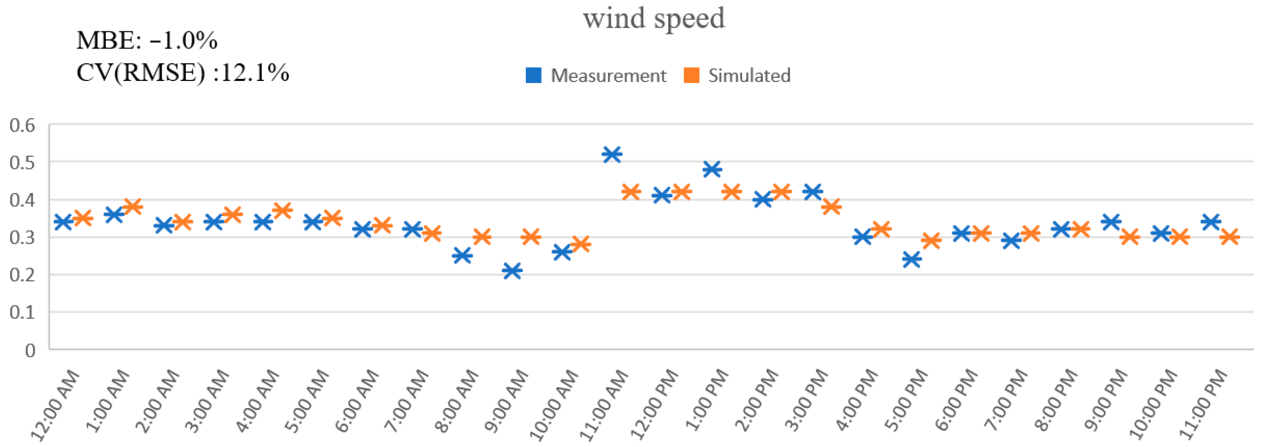
2.2.2. Microclimate Measurements and Validation
- (1)
- Honeybee’s simulation of indoor comfort is based on outdoor meteorological elements and does not offer a separate input interface for indoor data;
- (2)
- This study focused on performance comparisons between multiple schemes, emphasizing the relative improvement or degradation in performance rather than the building performance of a single scheme;
- (3)
- Since various factors influence buildings during operation, the load settings for building energy units can vary significantly, with no unified standard. Therefore, this study only explored the energy consumption of buildings under ideal conditions, examining the differences in energy consumption between various schemes and the correlation with building parameters.
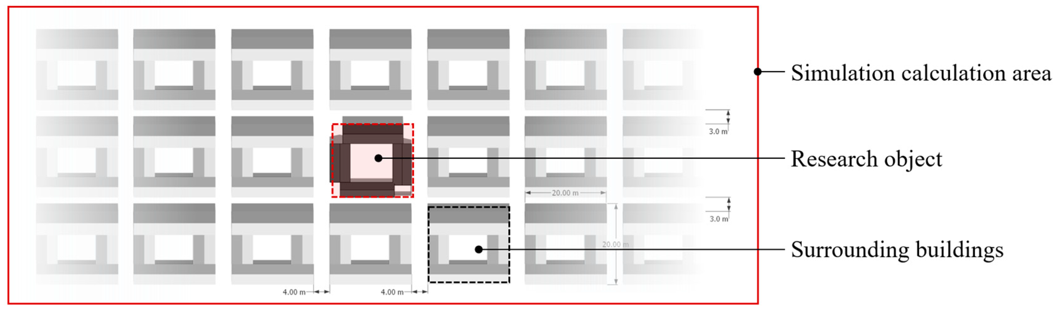
2.2.3. Baseline Courtyards Model and Environment Setup
2.3. Multi-Objective Genetic Optimization (MOGO) Based on Courtyards
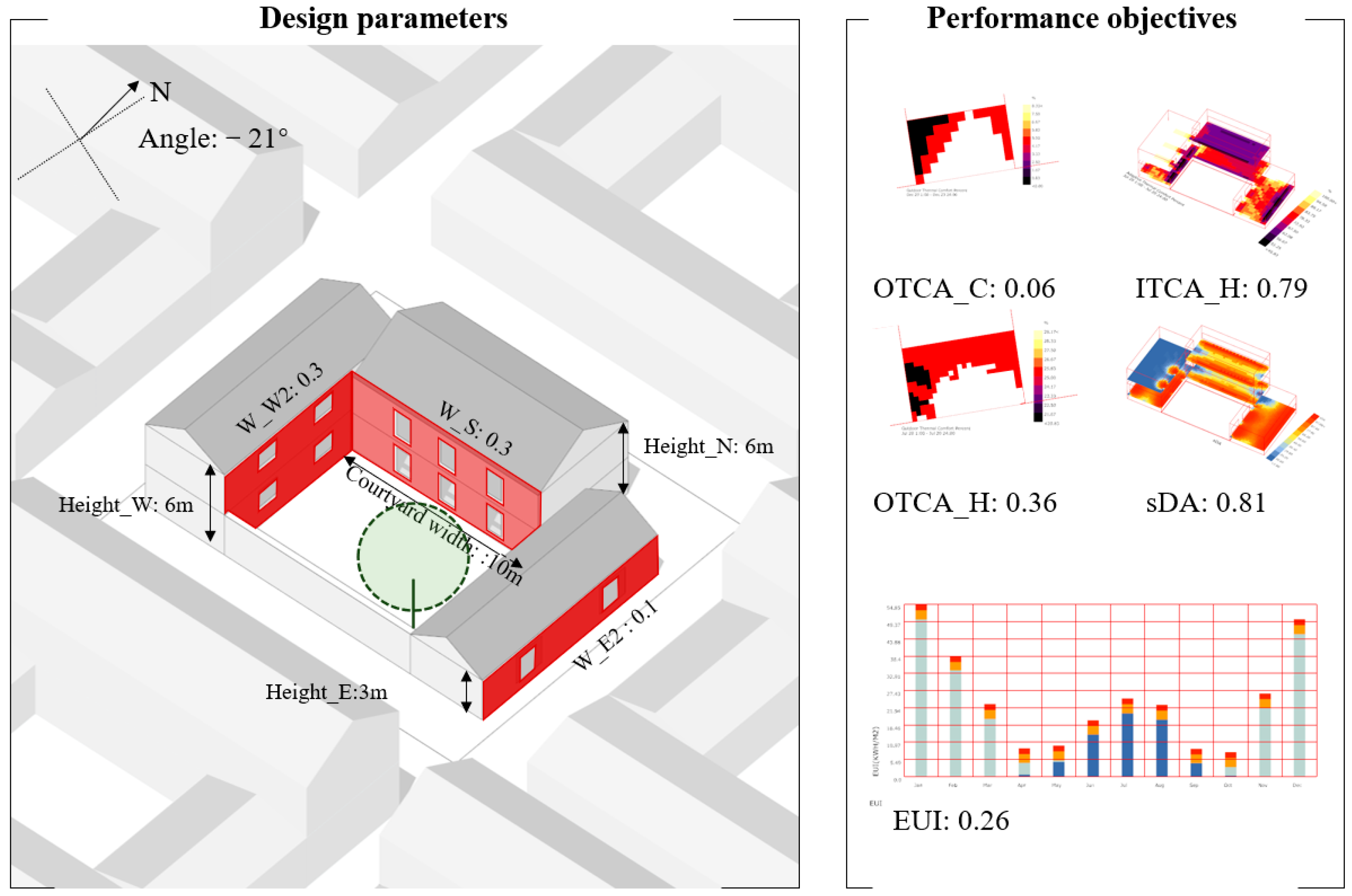
2.3.1. Design Parameters and Performance Objectives Selection
- (1)
- Outdoor Comfort: This criterion is based on Honeybee’s outdoor comfort autonomy modules, using PET (Physiological Equivalent Temperature) as the evaluation index. The goal is to maximize the proportion of time within the 5–31 °C threshold, a range deemed acceptable for cold regions according to related studies [27,30]. The analysis period aligns with the benchmark model from the previous stage, focusing on typical weeks in summer and winter (20–26 July and 23–29 December, respectively). The results are denoted as “OTCA_C” for winter and “OTCA_H” for summer.
- (2)
- Indoor Comfort: Similar to the outdoor comfort model, the indoor comfort autonomy modules assess the proportion of comfortable time under natural ventilation, utilizing the adaptive comfort model proposed by De Dear and Brager [31]. The analysis concentrates on the typical summer week (20–26 July). In northern China, where heating is provided from November to March, indoor comfort generally remains within comfort ranges under steady-state conditions, rendering further analysis of a typical winter week unnecessary. The results are represented by “ITCA_H”.
- (3)
- Indoor Illuminance: This criterion evaluates indoor lighting conditions over a year using spatial Daylight Autonomy (sDA) as the index. sDA measures the proportion of time in a year that achieves an illuminance level of 300 lux by the “Standard for Lighting Design of Buildings” [32]. The results are indicated by “sDA”.
- (4)
- Building Energy Consumption: Energy Use Intensity (EUI) was chosen as the evaluation standard, referring to the energy consumption per unit building area (kWh/m²) over one year. Since energy consumption values tend to be larger than other indicators, EUI was normalized to a range of 0–1 for easier comparison.
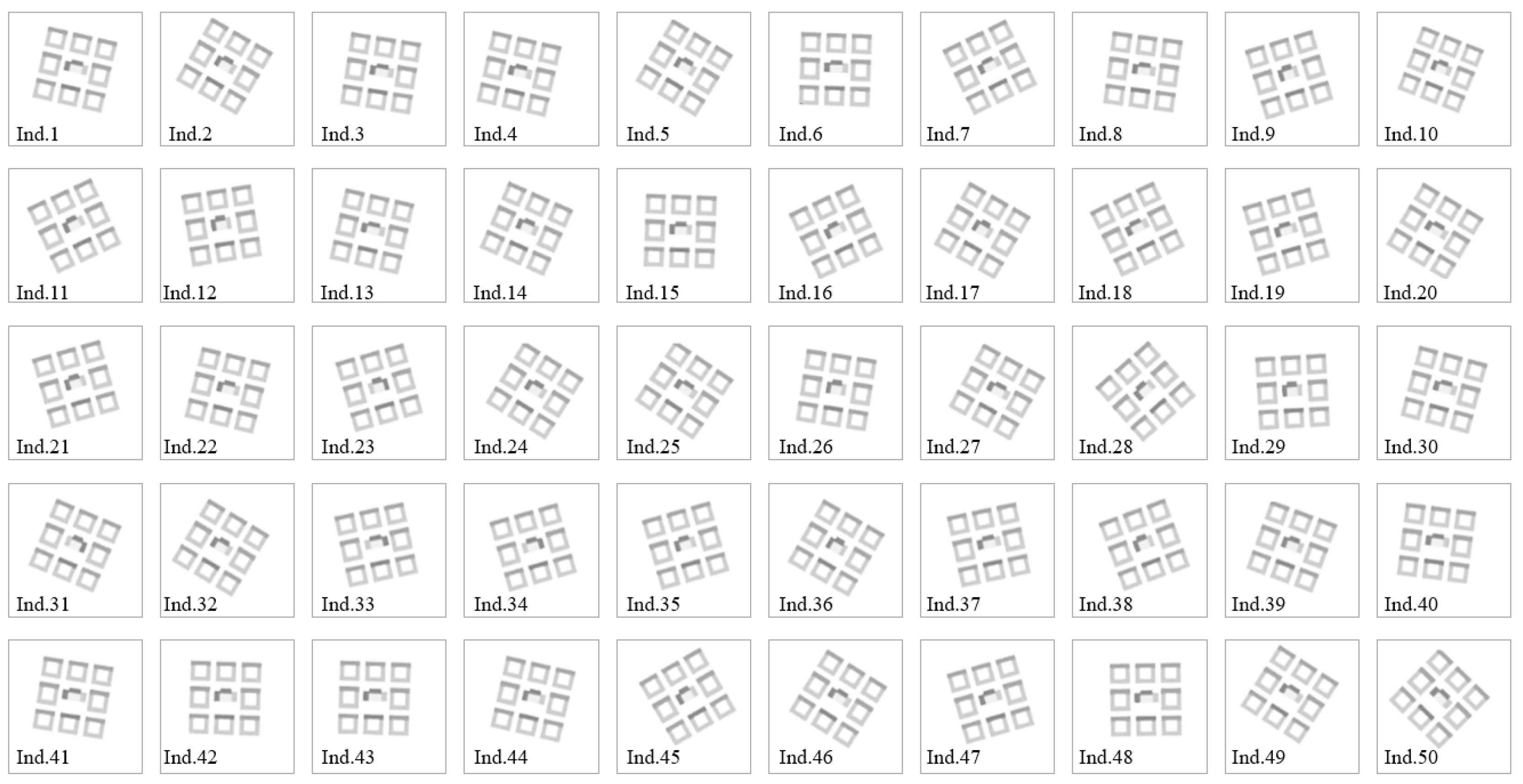
2.3.2. Simulation Generation Setup
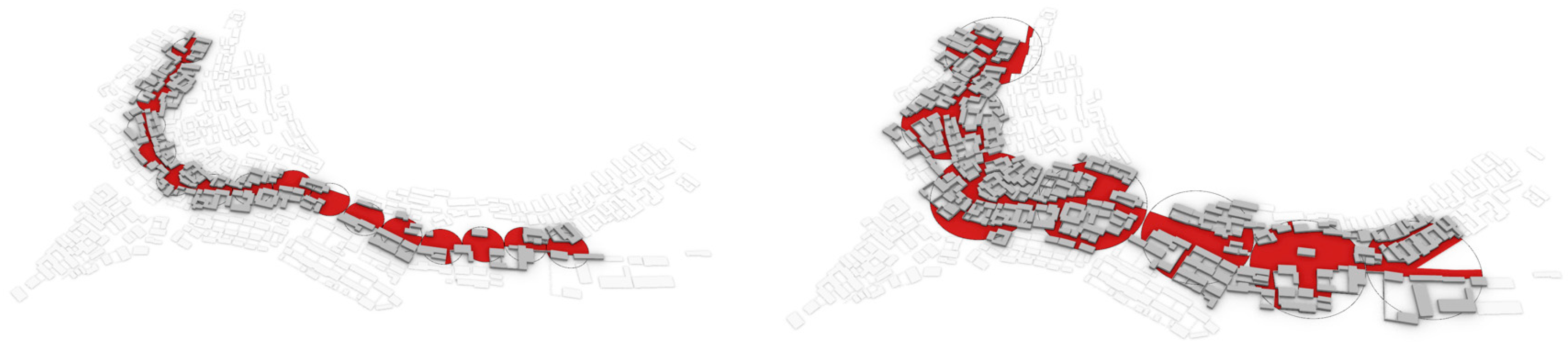
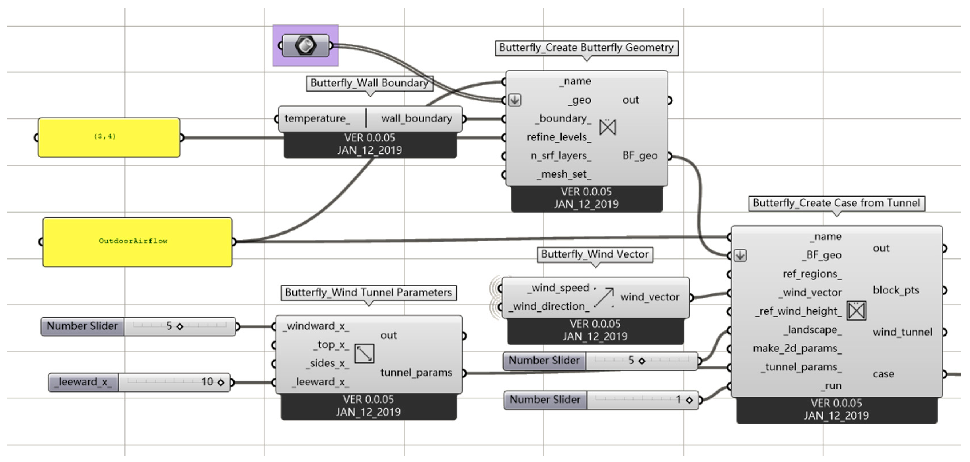
2.4. Simulation and Correlation Analysis of Wind and Thermal Environment Performance Based on Street Networks
2.5. Machine Learning Settings
2.5.1. Data Preprocessing
2.5.2. Data Splitting
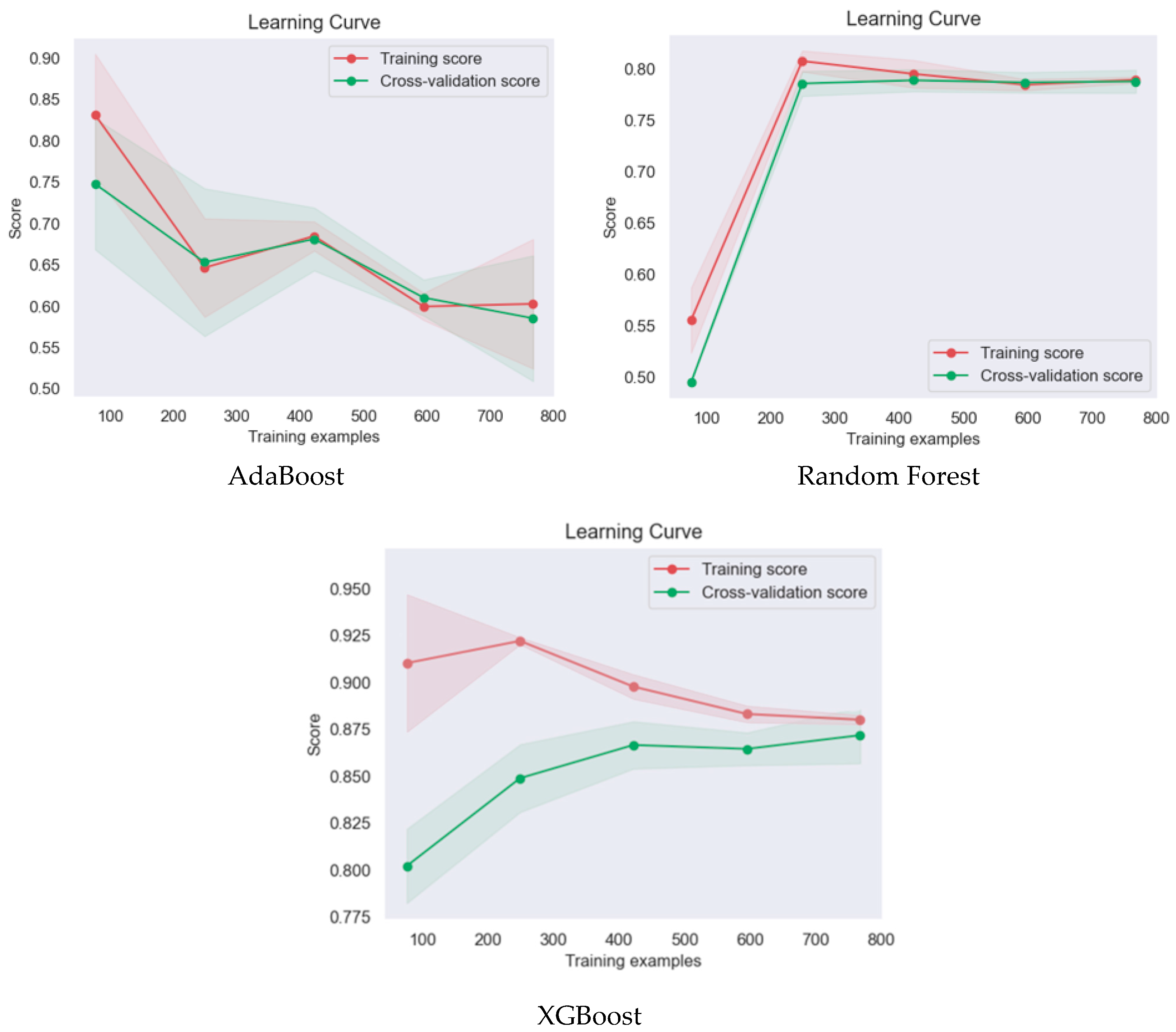
2.5.3. Algorithm Selection, Model Setting, and Validation of Model Training Accuracy
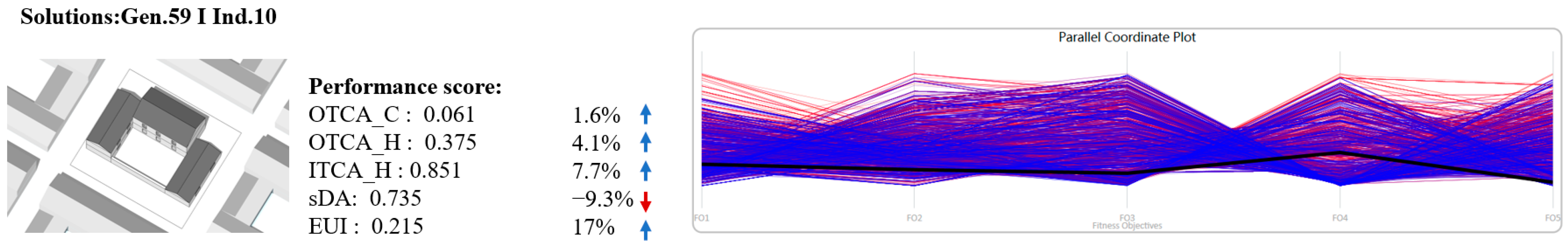
2.6. Solution Validation
3. Results
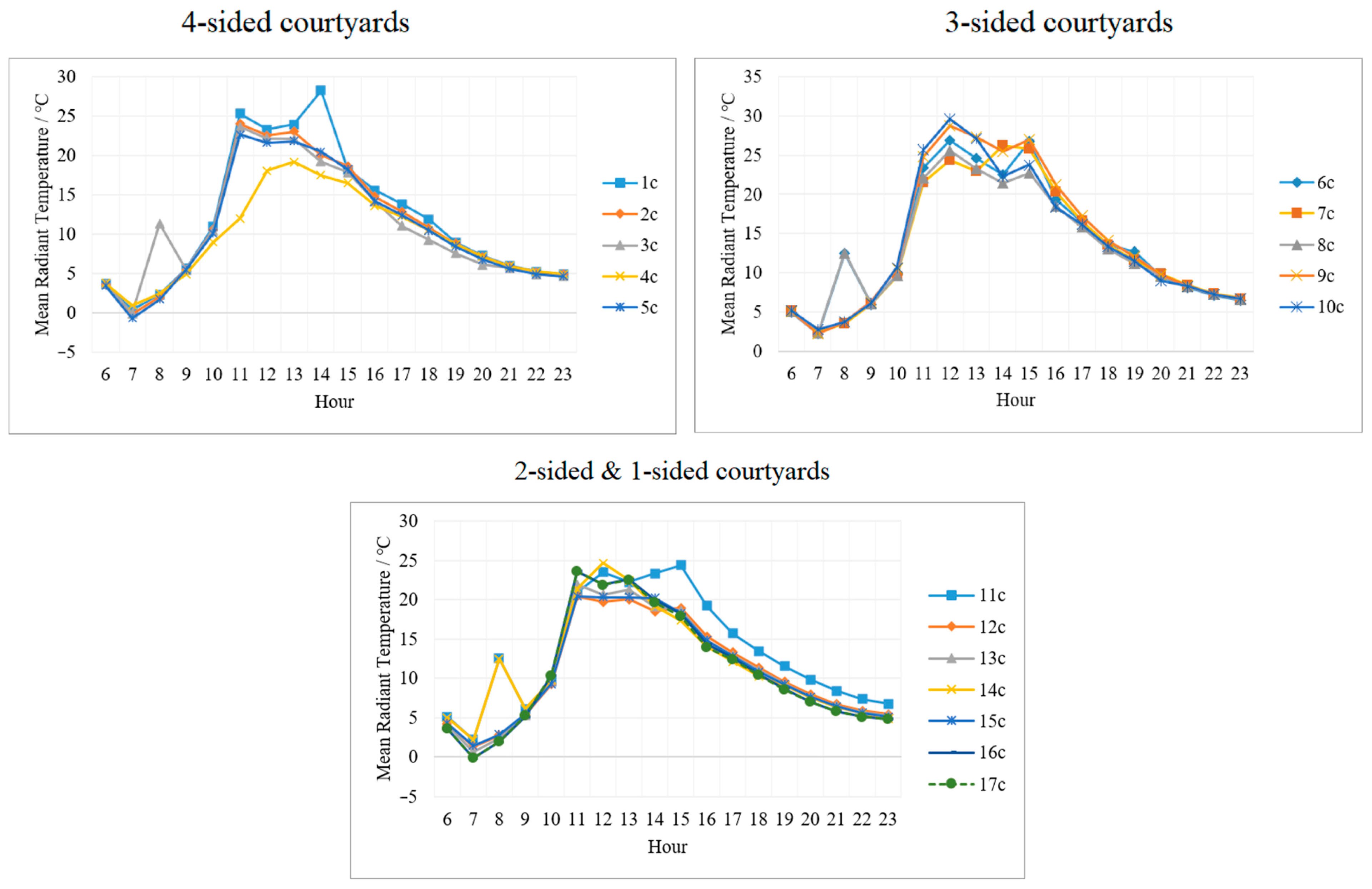
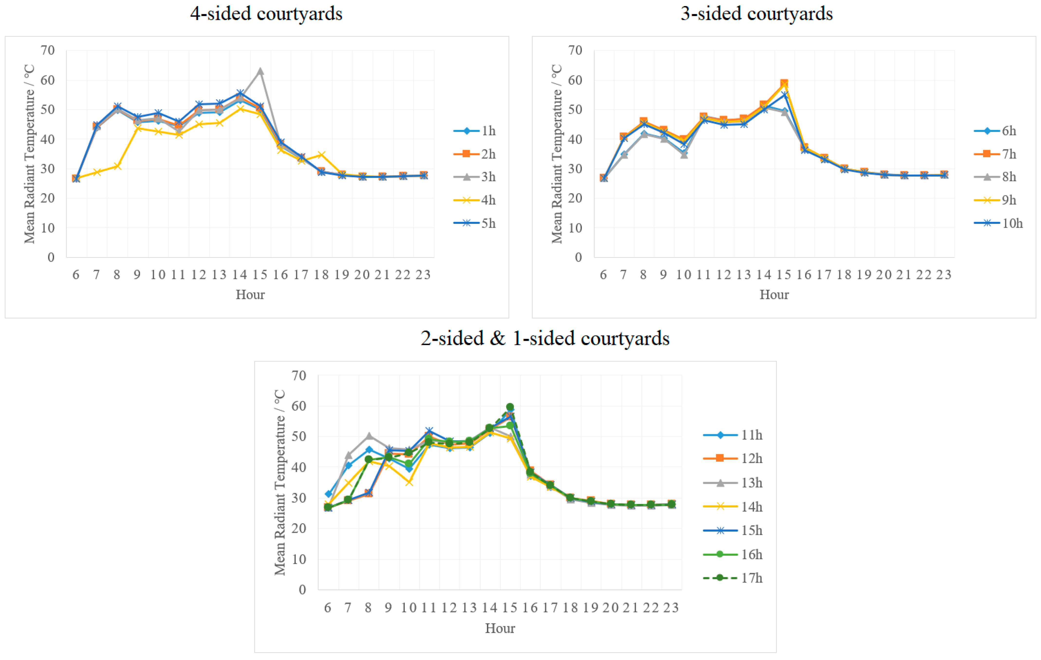
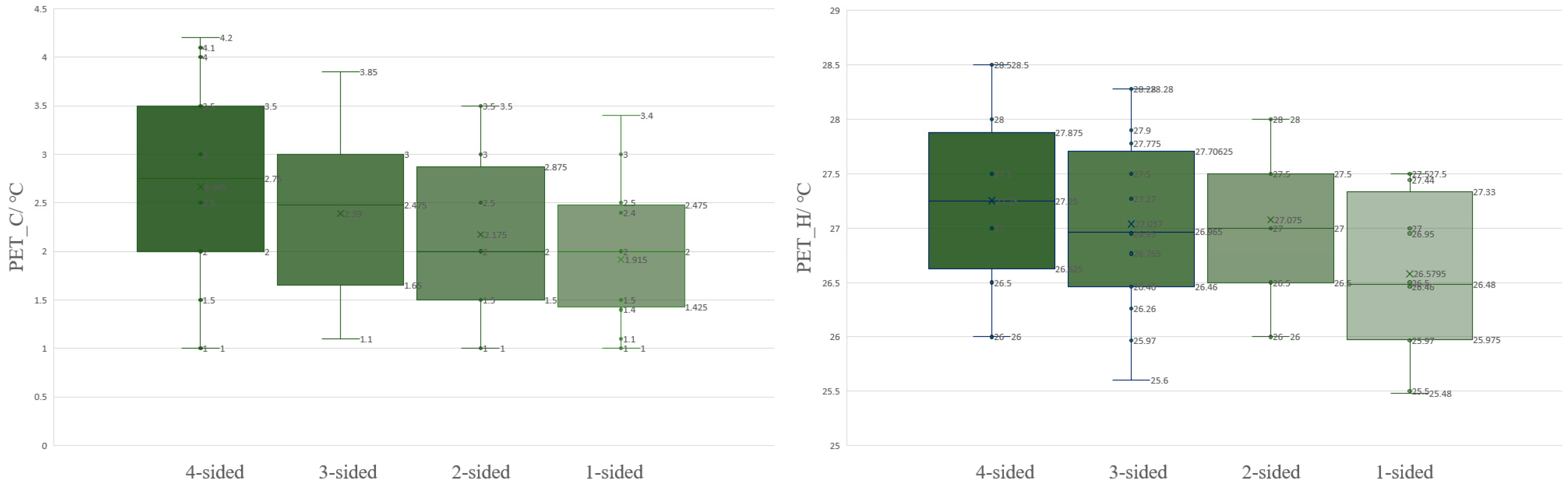
3.1. Baseline Model Selection
3.2. Simulation of Courtyard Performance
3.3. Simulation and Prediction Equation of Street Space Performance
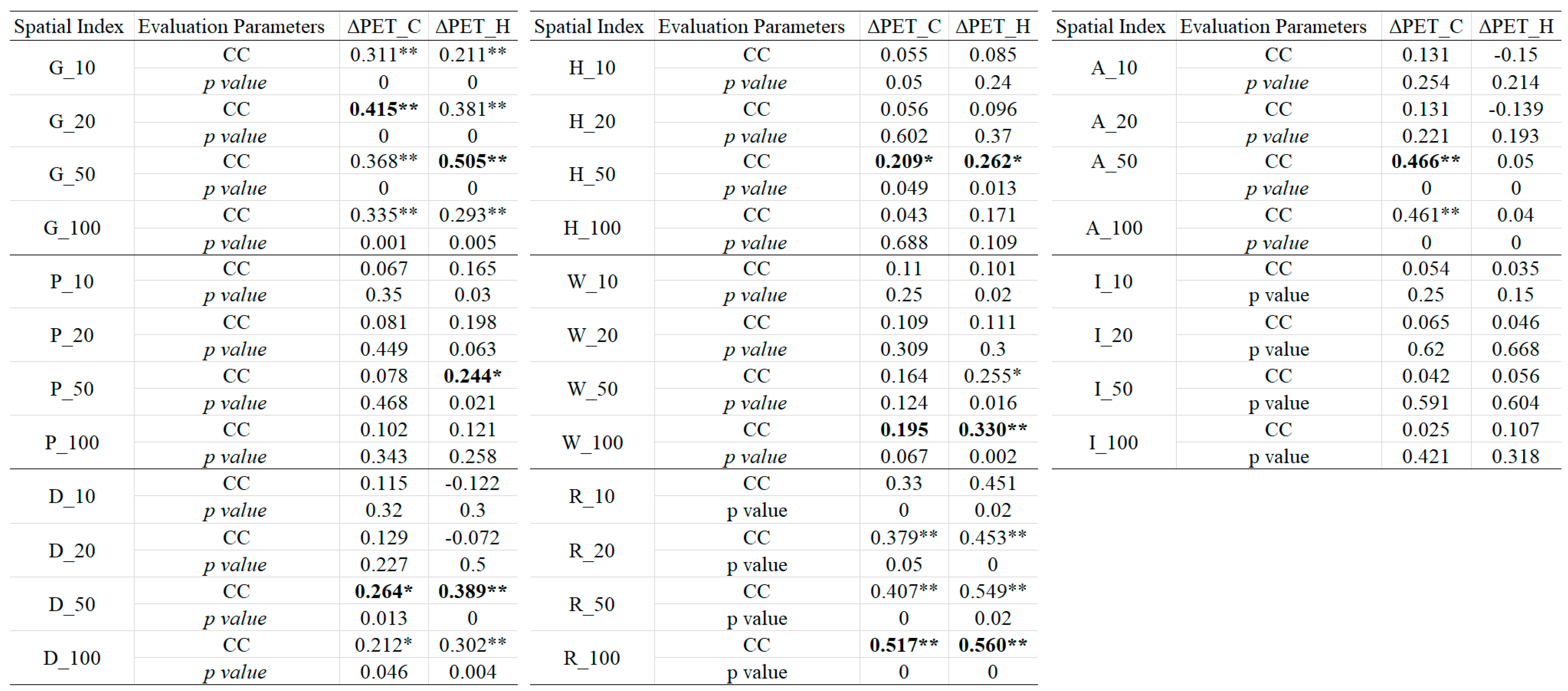
3.3.1. Analysis of Street Thermal Environment Performance
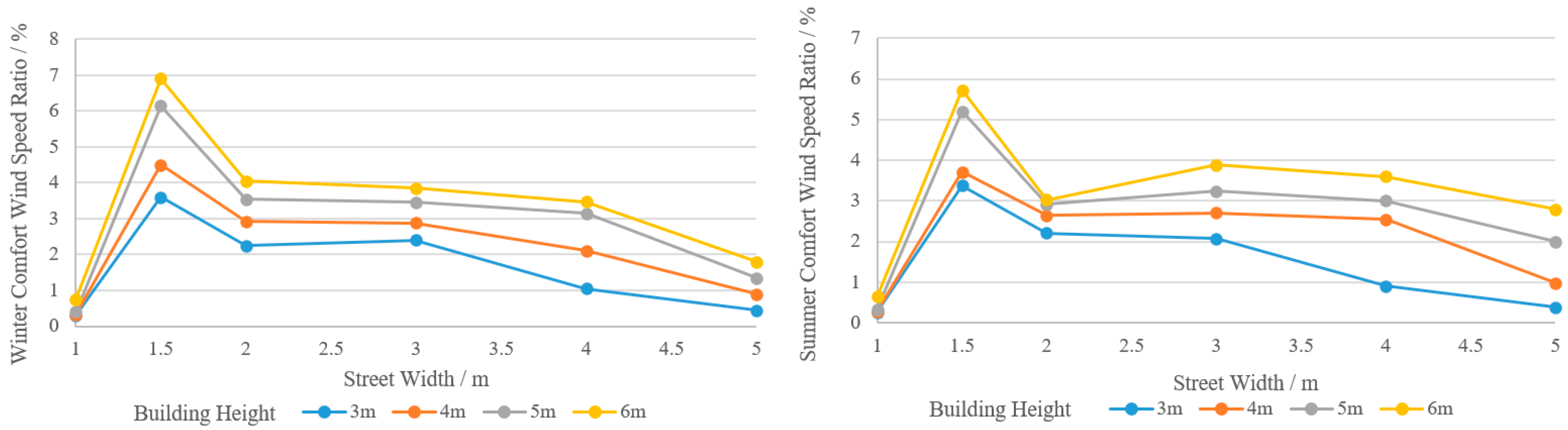
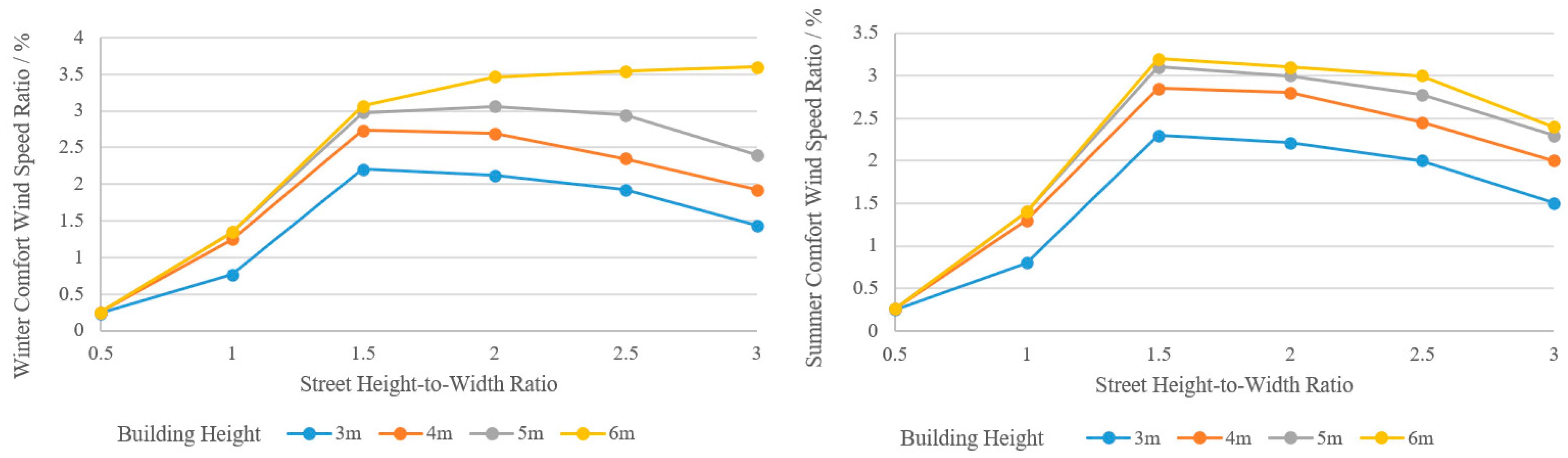
3.3.2. Analysis of Street Wind Environment Performance
3.4. Machine Learning Validation
3.4.1. Analysis of the Influence of Courtyard Design Parameters
3.4.2. Verification Results of Machine Learning Accuracy
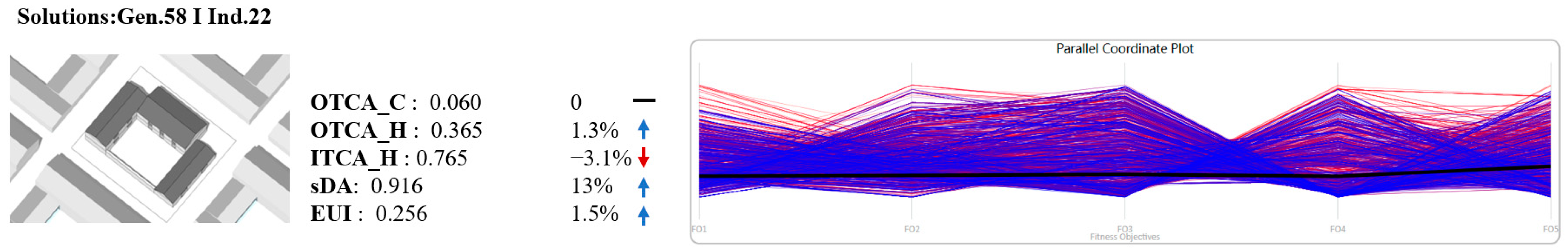
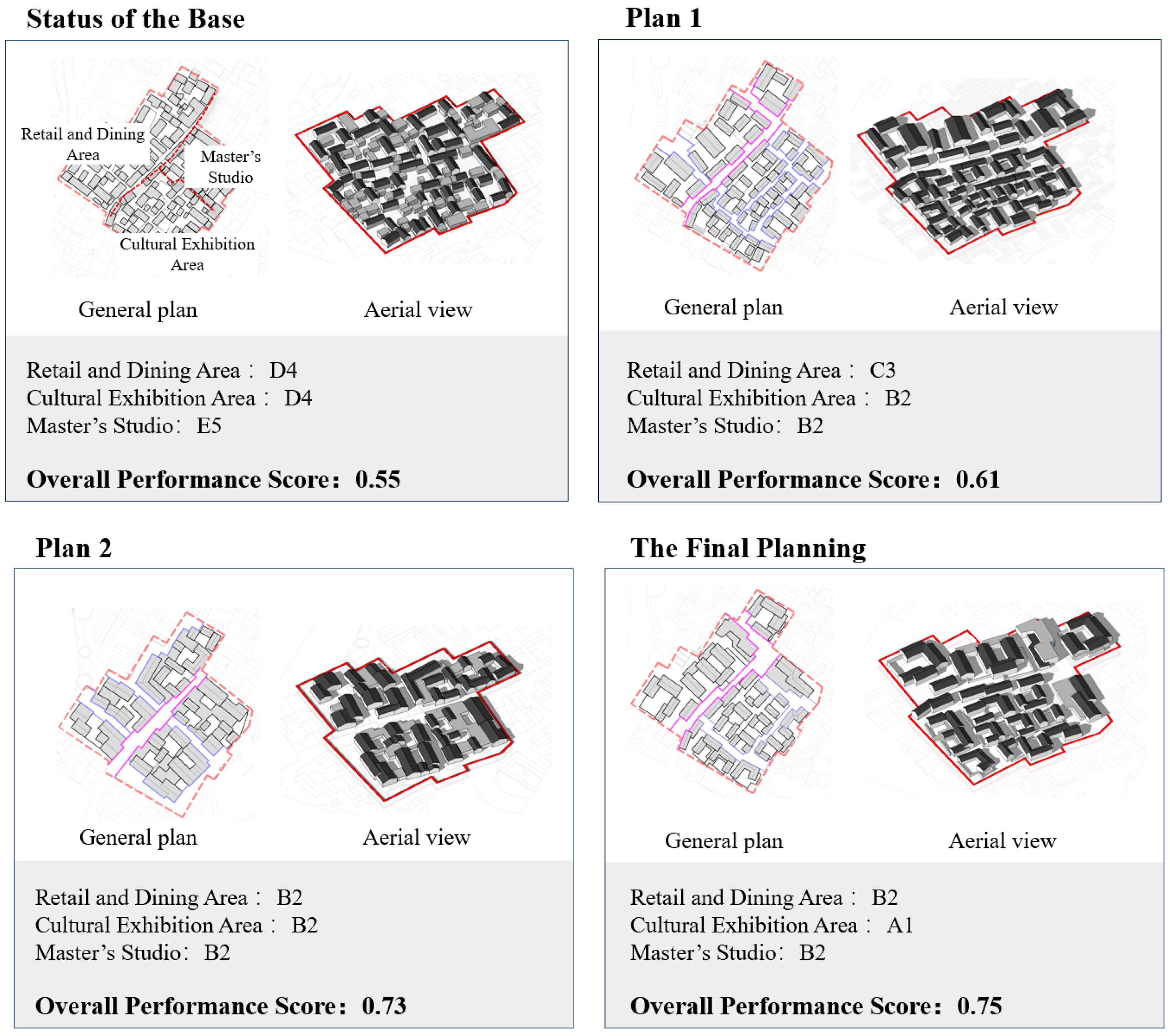
3.5. Application and Performance Analysis Statistics
4. Discussion
5. Conclusions
Author Contributions
Funding
Data Availability Statement
Conflicts of Interest
References
- Yuan, P.F.; Song, Y.; Lin, Y.; Beh, H.S.; Chao, Y.; Xiao, T.; Wu, Z. An architectural building cluster morphology generation method to perceive, derive, and form based on cyborg-physical wind tunnel (CPWT). Build. Environ. 2021, 203, 108045. [Google Scholar] [CrossRef]
- Yang, B.; Li, X.; Liu, Y.; Chen, L.; Guo, R.; Wang, F.; Yan, K. Comparison of models for predicting winter individual thermal comfort based on machine learning algorithms. Build. Environ. 2022, 215, 108970. [Google Scholar] [CrossRef]
- Yan, H.; Yan, K.; Ji, G. Optimization and prediction in the early design stage of office buildings using genetic and XGBoost algorithms. Build. Environ. 2022, 218, 109081. [Google Scholar] [CrossRef]
- Sakiyama, N.R.M.; Carlo, J.C.; Mazzaferro, L.; Garrecht, H. Building optimization through a parametric design platform: Using sensitivity analysis to improve a radial-based algorithm performance. Sustainability 2021, 13, 5739. [Google Scholar] [CrossRef]
- Fan, Z.; Liu, M.; Tang, S.; Zong, X. Multi-objective optimization for gymnasium layout in early design stage: Based on genetic algorithm and neural network. Build. Environ. 2024, 258, 111577. [Google Scholar] [CrossRef]
- Al-Homoud, M.S. Optimum thermal design of office buildings. Int. J. Energy Res. 1997, 21, 941–957. [Google Scholar] [CrossRef]
- Coley, D.A.; Schukat, S. Low-energy design: Combining computer-based optimisation and human judgement. Build. Environ. 2022, 37, 1241–1247. [Google Scholar] [CrossRef]
- Hauglustaine, J.M.; Azar, S. Interactive tool aiding to optimise the building envelope during the sketch design. In Proceedings of the Seventh International IBPSA Conference, Rio de Janeiro, Brazil, 13–15 August 2001; pp. 387–394. [Google Scholar]
- Dong, Y.; Sun, C.; Han, Y.; Liu, Q. Intelligent optimization: A novel framework to automatize multi-objective optimization of building daylighting and energy performances. J. Build. Eng. 2021, 43, 102804. [Google Scholar] [CrossRef]
- Tian, Z.; Zhang, X.; Jin, X.; Zhou, X.; Si, B.; Shi, X. Towards adoption of building energy simulation and optimization for passive building design: A survey and a review. Energy Build. 2018, 158, 1306–1316. [Google Scholar] [CrossRef]
- Sun, P.; Yan, F.; He, Q.; Liu, H. The Development of an Experimental Framework to Explore the Generative Design Preference of a Machine Learning-Assisted Residential Site Plan Layout. Land 2023, 12, 1776. [Google Scholar] [CrossRef]
- Kim, S.; Lee, J.; Jeong, K.; Lee, J.; Hong, T.; An, J. Automated door placement in architectural plans through combined deep-learning networks of ResNet-50 and Pix2Pix-GAN. Expert Syst. Appl. 2024, 244, 122932. [Google Scholar] [CrossRef]
- Mostafavi, F.; Tahsildoost, M.; Zomorodian, Z.S.; Shahrestani, S.S. An interactive assessment framework for residential space layouts using pix2pix predictive model at the early-stage building design. Smart Sustain. Built Environ. 2024, 13, 809–827. [Google Scholar] [CrossRef]
- Fan, C.; Xiao, F.; Yan, C.; Liu, C.; Li, Z.; Wang, J. A novel methodology to explain and evaluate data-driven building energy performance models based on interpretable machine learning. Appl. Energy 2019, 235, 1551–1560. [Google Scholar] [CrossRef]
- Olu-Ajayi, R.; Alaka, H.; Sulaimon, I.; Sunmola, F.; Ajayi, S. Machine learning for energy performance prediction at the design stage of buildings. Energy Sustain. Dev. 2022, 66, 12–25. [Google Scholar] [CrossRef]
- Seyedzadeh, S.; Rahimian, F.P.; Oliver, S.; Rodriguez, S.; Glesk, I. Machine learning modelling for predicting non-domestic buildings energy performance: A model to support deep energy retrofit decision-making. Appl. Energy 2020, 279, 115908. [Google Scholar] [CrossRef]
- Ahmad, T.; Chen, H.; Huang, R.; Yabin, G.; Wang, J.; Shair, J. Supervised based machine learning models for short, medium and long-term energy prediction in distinct building environment. Energy 2018, 158, 17–32. [Google Scholar] [CrossRef]
- Liu, Z.; Wu, D.; Liu, Y.; Han, Z.; Lun, L.; Gao, J. Accuracy analyses and model comparison of machine learning adopted in building energy consumption prediction. Energy Explor. Exploit. 2019, 37, 1426–1451. [Google Scholar] [CrossRef]
- Lin, C.H.; Tsay, Y.S. A metamodel based on intermediary features for daylight performance prediction of façade design. Build. Environ. 2021, 206, 108371. [Google Scholar] [CrossRef]
- Mo, H.; Sun, H.; Liu, J.; Wei, S. Developing window behavior models for residential buildings using XGBoost algorithm. Energy Build. 2019, 205, 109564. [Google Scholar] [CrossRef]
- Tien, P.W.; Wei, S.; Darkwa, J.; Wood, C.; Calautit, J.K. Machine learning and deep learning methods for enhancing building energy efficiency and indoor environmental quality—A review. Energy AI 2022, 10, 100198. [Google Scholar] [CrossRef]
- Ngarambe, J.; Irakoze, A.; Yun, G.Y.; Kim, G. Comparative performance of machine learning algorithms in the prediction of indoor daylight illuminances. Sustainability 2020, 12, 4471. [Google Scholar] [CrossRef]
- Alawadi, S.; Mera, D.; Fernández-Delgado, M.; Alkhabbas, F.; Olsson, C.M.; Davidsson, P. A comparison of machine learning algorithms for forecasting indoor temperature in smart buildings. Energy Syst. 2020, 13, 689–705. [Google Scholar] [CrossRef]
- Teshnehdel, S.; Mirnezami, S.; Saber, A.; Pourzangbar, A.; Olabi, A.G. Data-driven and numerical approaches to predict thermal comfort in traditional courtyards. Sustain. Energy Technol. Assess. 2020, 37, 100569. [Google Scholar] [CrossRef]
- Guo, J.; Li, M.; Jin, Y.; Shi, C.; Wang, Z. Energy Prediction and Optimization Based on Sequential Global Sensitivity Analysis: The Case Study of Courtyard-Style Dwellings in Cold Regions of China. Buildings 2022, 12, 1132. [Google Scholar] [CrossRef]
- Chen, X.; Xue, P.; Liu, L.; Gao, L.; Liu, J. Outdoor thermal comfort and adaptation in severe cold area: A longitudinal survey in Harbin, China. Build. Environ. 2018, 143, 548–560. [Google Scholar] [CrossRef]
- Yuan, T.; Hong, B.; Qu, H.; Liu, A.; Zheng, Y. Outdoor thermal comfort in urban and rural open spaces: A comparative study in China’s cold region. Urban Clim. 2023, 49, 101501. [Google Scholar] [CrossRef]
- Du, J.; Sun, C.; Xiao, Q.; Chen, X.; Liu, J. Field assessment of winter outdoor 3-D radiant environment and its impact on thermal comfort in a severely cold region. Sci. Total Environ. 2020, 709, 136175. [Google Scholar] [CrossRef] [PubMed]
- Krüger, E.L.; Minella, F.O.; Matzarakis, A. Comparison of different methods of estimating the mean radiant temperature in outdoor thermal comfort studies. Int. J. Biometeorol. 2014, 58, 1727–1737. [Google Scholar] [CrossRef]
- Mi, J.; Hong, B.; Zhang, T.; Huang, B.; Niu, J. Outdoor thermal benchmarks and their application to climate–responsive designs of residential open spaces in a cold region of China. Build. Environ. 2020, 169, 106592. [Google Scholar] [CrossRef]
- De Dear, R.; Schiller Brager, G. The adaptive model of thermal comfort and energy conservation in the built environment. Int. J. Biometeorol. 2001, 45, 100–108. [Google Scholar] [CrossRef]
- GB/T50034-2024; Standard for Lighting Design of Buildings. China Architecture & Building Press: Beijing, China, 2024.
- Zhang, L.; Zhang, L.; Wang, Y. Shape optimization of free-form buildings based on solar radiation gain and space efficiency using a multi-objective genetic algorithm in the severe cold zones of China. Sol. Energy 2016, 132, 38–50. [Google Scholar] [CrossRef]
- Azari, R.; Garshasbi, S.; Amini, P.; Rashed-Ali, H.; Mohammadi, Y. Multi-objective optimization of building envelope design for life cycle environmental performance. Energy Build. 2016, 126, 524–534. [Google Scholar] [CrossRef]
- Gossard, D.; Lartigue, B.; Thellier, F. Multi-objective optimization of a building envelope for thermal performance using genetic algorithms and artificial neural network. Energy Build. 2013, 67, 253–260. [Google Scholar] [CrossRef]
- Jalali, Z.; Noorzai, E.; Heidari, S. Design and optimization of form and facade of an office building using the genetic algorithm. Sci. Technol. Built Environ. 2020, 26, 128–140. [Google Scholar] [CrossRef]
- Wang, Z.; Rangaiah, G.P. Application and analysis of methods for selecting an optimal solution from the Pareto-optimal front obtained by multiobjective optimization. Ind. Eng. Chem. Res. 2017, 56, 560–574. [Google Scholar] [CrossRef]
- Wright, J.A.; Brownlee, A.; Mourshed, M.M.; Wang, M. Multi-objective optimization of cellular fenestration by an evolutionary algorithm. J. Build. Perform. Simul. 2014, 7, 33–51. [Google Scholar] [CrossRef]
- Wang, W.; Zmeureanu, R.; Rivard, H. Applying multi-objective genetic algorithms in green building design optimization. Build. Environ. 2005, 40, 1512–1525. [Google Scholar] [CrossRef]
- Rosso, F.; Ciancio, V.; Dell’Olmo, J.; Salata, F. Multi-objective optimization of building retrofit in the Mediterranean climate by means of genetic algorithm application. Energy Build. 2020, 216, 109945. [Google Scholar] [CrossRef]
- Satrio, P.; Mahlia, T.M.I.; Giannetti, N.; Saito, K. Optimization of HVAC system energy consumption in a building using artificial neural network and multi-objective genetic algorithm. Sustain. Energy Technol. Assess. 2019, 35, 48–57. [Google Scholar]
- Murakami, S.; Zeng, J.; Hayashi, T. CFD analysis of wind environment around a human body. J. Wind Eng. Ind. Aerodyn. 1999, 83, 393–408. [Google Scholar] [CrossRef]
- JGJT449-2018; Green Performance Calculation Standard for Civil Buildings. China Architecture & Building Press: Beijing, China, 2018.
- Mousa, W.A.Y.; Lang, W.; Auer, T. Assessment of the impact of window screens on indoor thermal comfort and energy efficiency in a naturally ventilated courtyard house. Archit. Sci. Rev. 2017, 60, 382–394. [Google Scholar] [CrossRef]
- López-Cabeza, V.P.; Carmona-Molero, F.J.; Rubino, S.; Rivera-Gómez, C.; Fernández-Nieto, E.D.; Galán-Marín, C.; Chacón-Rebollo, T. Modelling of surface and inner wall temperatures in the analysis of courtyard thermal performances in Mediterranean climates. J. Build. Perform. Simul. 2021, 14, 181–202. [Google Scholar] [CrossRef]
- Ghorbani Naeini, H.; Norouziasas, A.; Piraei, F.; Kazemi, M.; Kazemi, M.; Hamdy, M. Impact of building envelope parameters on occupants’ thermal comfort and energy use in courtyard houses. Archit. Eng. Des. Manag. 2023, 1–27. [Google Scholar] [CrossRef]
- Che, W.W.; Tso, C.Y.; Sun, L.; Ip, D.Y.; Lee, H.; Chao, C.Y.; Lau, A.K. Energy consumption, indoor thermal comfort and air quality in a commercial office with retrofitted heat, ventilation and air conditioning (HVAC) system. Energy Build. 2019, 201, 202–215. [Google Scholar] [CrossRef]
- Muhaisen, A.S. Shading simulation of the courtyard form in different climatic regions. Build. Environ. 2006, 41, 1731–1741. [Google Scholar] [CrossRef]


| Elevation (m) | <50 | 50–100 | 100–200 | 200–500 | >500 |
|---|---|---|---|---|---|
| Number of Villages | 159 | 64 | 134 | 140 | 22 |
| Index | Energy Model Parameters |
|---|---|
| Wall | 5 mm Cement mortar + 370 mm Fired claybrick U-value = 1.72 W·m−2·K−1 |
| Floor | 10 mm Ceramic tile + 100 mm Concrete + 1500 mm Plain soil compaction U-value = 0.47 W·m−2·K−1 |
| Roof | Color steel plate+ 10 mm Asphalt felt +10 mm Grass clay + 200 mm Cement mortar U-value = 1.94 W·m−2·K−1 |
| Glazing | Wooden Glass U-value = 5.03 W·m−2·K−1 SHGC = 0.6 |
| Shading | Not applied |
| Equipment loads per area | 3.7 W·m−2 |
| Infiltration rate per area | 0.4 cfm/sf facade @ 75 Pa |
| Lighting density per area | 11.8 W·m−2 |
| Num. of people per area | 0.03 people·m−2 |
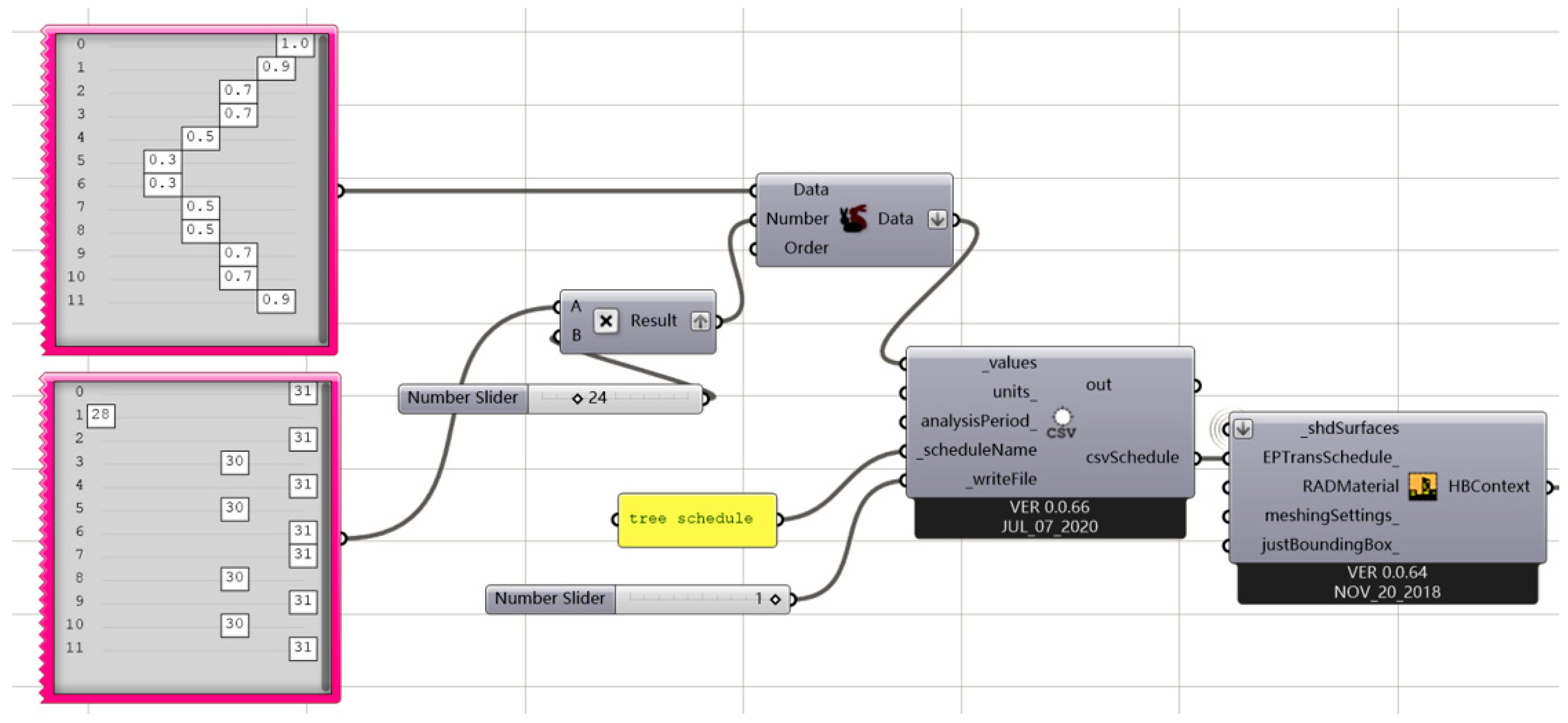
| Schedules | Default Honeybee residential schedules /The Schedule for controlling tree porosity |
| HVAC | Ideal mechanical system |
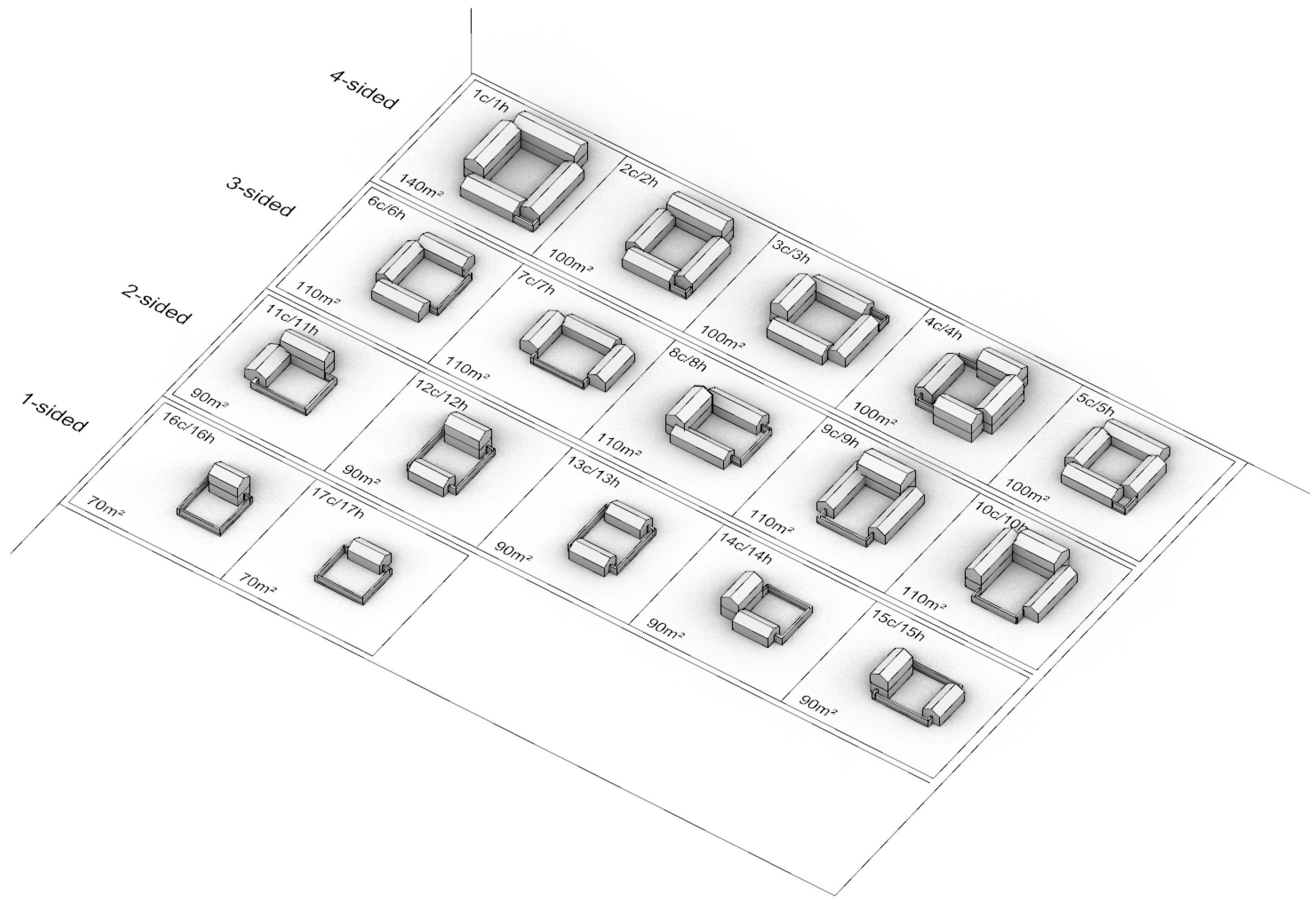
| Classification | No. | Orientation | No. of 2-Storey Buildings | Category Code ** | Total Categories | ||
|---|---|---|---|---|---|---|---|
| Traditional Courtyards (105) | 4-sided | 13 | North–South | 0 | 5c/5h | 17 | |
| 1 | 2c/2h | ||||||
| 2 | 1c/1h | ||||||
| East–West | 1 | 3c/3h | |||||
| 3 | 4c/4h | ||||||
| 3-sided | 45 | North–South | 0 | 7c/7h | |||
| 1 | 9c/9h | ||||||
| 2 | 10c/10h | ||||||
| East–West | 0 | 6c/6h | |||||
| 1 | 8c/8h | ||||||
| 2-sided | 33 | North–South | Central * | 0 | 13c/13h | ||
| 1 | 12c/12h | ||||||
| East | 1 | 11c/11h | |||||
| East–West | Central | 1 | 15c/15h | ||||
| East | 1 | 14c/14h | |||||
| 1-sided | 14 | North–South | 0 | 17c/17h | |||
| East–West | 1 | 16c/16h | |||||
| Design Variables | Unit | Scope |
|---|---|---|
| Courtyard width | m | [8, 13] |
| Standard floor height | m | [2.6, 4.1] |
| Orientation | ° | [−45, 45] |
| Secondary-house Floor Control | - | [−1, 1] |
| Window-to-wall ratio | - | [0, 0.35] |
| Performance Objectives | Analysis Period | The Acceptable Range | Scope | |
|---|---|---|---|---|
| Outdoor Comfort | OTCA_C | Typical Week in Winter | >5 °C | [0, 1] |
| OTCA_H | Typical Week in Summer | <32 °C | [0, 1] | |
| Indoor Comfort | ITCA_H | Typical Week in Summer | <32 °C | [0, 1] |
| sDA | 1 year | >300 l× | [0, 1] | |
| Building energy consumption | EUI | 1 year | - | [0, 1] |
| Population | |
|---|---|
| Generation size | 50 |
| Generation count | 60 |
| Algorithm parameters | |
| Crossover probability | 0.9 |
| Mutation probability | 1/n |
| Crossover distribution index | 20 |
| Mutation distribution index | 20 |
| Random seed | 1 |
| Outdoor_C | Outdoor_H | Indoor_H | Indoor_sDA | EUI | |
|---|---|---|---|---|---|
| Cluster 1/Individual. 1 | 0.052194 | 0.353481 | 0.892496 | 0.893248 | 0.372975 |
| Cluster 2/Individual. 6 | 0.060127 | 0.368541 | 0.793157 | 0.972145 | 0.265634 |
| Cluster 3/Individual. 3 | 0.057044 | 0.361921 | 0.739375 | 0.792245 | 0.393248 |
| Cluster 4/Individual. 5 | 0.069542 | 0.349952 | 0.897124 | 0.521406 | 0.391205 |
| Cluster 5/Individual. 11 | 0.068231 | 0.365781 | 0.926355 | 0.575702 | 0.376893 |
| Cluster 6/Individual. 8 | 0.067198 | 0.354203 | 0.885853 | 0.529257 | 0.389754 |
| Generations | sDA Value | Performance Label | |
|---|---|---|---|
| Pareto Front Solutions | 40–59 | >0.7 | A1 |
| 20–39 | >0.7 | B2 | |
| 0–19 | >0.7 | C3 | |
| 0–59 | <0.7 | D4 | |
| Non-Front Solutions | 0–59 | >0.7 | E5 |
| 0–59 | <0.7 | F6 |
| Index/Performance Rating | Outdoor Comfort | Indoor Comfort | Building Energy Consumption /EUI | Prediction Accuracy | ||
|---|---|---|---|---|---|---|
| Outdoor_C Simulation | Outdoor_H Simulation | Indoor_H Simulation | Indoor_sDA Simulation | |||
| 1/A | 0.051136 | 0.358759 | 0.892034 | 0.89998 | 0.372426 | 89% |
| Optimization percentage |  −27% −27% | −1% |  12% 12% | 11% | 42% | |
| 2/B | 0.069129 | 0.365641 | 0.780046 | 0.79998 | 0.317511 | 82% |
| Optimization percentage | 15% | 1% | −2% | −2% | 19% | |
| 3/C | 0.060938 | 0.362153 | 0.791221 | 0.98 | 0.262619 | 81% |
| Optimization percentage | - | - | - | 12% | - | |
| 4/D | 0.065476 | 0.35846 | 0.91218 | 0.53334 | 0.385004 | 75% |
| Optimization percentage | 8% | −1% | 15% | −33% | 46% | |
| 5/E | 0.057044 | 0.361921 | 0.739375 | 0.79998 | 0.390826 | 82% |
| Optimization percentage | −5% | - | −8% | −2% | 50% | |
| 6/F | 0.056551 | 0.351798 | 0.717885 | 0.78877 | 0.415123 | 88% |
| Optimization percentage | −5% | −3% | −11% | −2% | 57% | |
Disclaimer/Publisher’s Note: The statements, opinions and data contained in all publications are solely those of the individual author(s) and contributor(s) and not of MDPI and/or the editor(s). MDPI and/or the editor(s) disclaim responsibility for any injury to people or property resulting from any ideas, methods, instructions or products referred to in the content. |
© 2024 by the authors. Licensee MDPI, Basel, Switzerland. This article is an open access article distributed under the terms and conditions of the Creative Commons Attribution (CC BY) license (https://creativecommons.org/licenses/by/4.0/).
Share and Cite
Xu, Z.; Li, X.; Sun, B.; Wen, Y.; Tang, P. Evaluation and Optimization of Traditional Mountain Village Spatial Environment Performance Using Genetic and XGBoost Algorithms in the Early Design Stage—A Case Study in the Cold Regions of China. Buildings 2024, 14, 2796. https://doi.org/10.3390/buildings14092796
Xu Z, Li X, Sun B, Wen Y, Tang P. Evaluation and Optimization of Traditional Mountain Village Spatial Environment Performance Using Genetic and XGBoost Algorithms in the Early Design Stage—A Case Study in the Cold Regions of China. Buildings. 2024; 14(9):2796. https://doi.org/10.3390/buildings14092796
Chicago/Turabian StyleXu, Zhixin, Xiaoming Li, Bo Sun, Yueming Wen, and Peipei Tang. 2024. "Evaluation and Optimization of Traditional Mountain Village Spatial Environment Performance Using Genetic and XGBoost Algorithms in the Early Design Stage—A Case Study in the Cold Regions of China" Buildings 14, no. 9: 2796. https://doi.org/10.3390/buildings14092796