Quantifying and Rating the Energy Resilience Performance of Buildings Integrated with Renewables in the Nordics under Typical and Extreme Climatic Conditions

Abstract

The future buildings and society need to be resilient. This article aims to propose a novel concept of the energy resilience framework and implement a color-based rating system to quantify and rate the energy resilience performance of buildings in Nordic climates. The objective is to conduct a comparative analysis between old (1970s) and new (2020s) single-family buildings integrated with renewable energy sources and storage, assessing their energy resilience performance for heating during power outages, under extreme and typical climatic conditions. The study utilizes dynamic simulation of the buildings and renewable energy systems, conducting parametric studies to calculate proposed resilience indicators and rate their resilience performance, employing both passive and active methods. The total costs of the design variables are also calculated for economic evaluation. Given the complexities arising from climate change, the article uses a simplified method to synthesize regional climate to consider extreme climate change impacts on energy resilience performance. For the old building lacking PV, the robustness duration increased from 1 h to 3 h, and the degree of disruption (DoD) varied from 0.545 to 0.3 in extreme cold to warm climate scenarios, with the higher DoD number indicating worse performance. The impact of the season within the same climate scenario is also evident, as the habitability and robustness durations increased during spring compared to winter. The resilience improved with PV and battery. The new building showed that the robustness duration increased from 3 to 15 h, habitability durations increased, and the DoD varied from 0.496 to 0.22 from extreme cold to warm climates without renewables and storage. With the integration of PV and battery, the new building was able to achieve a lower DoD and better performance with lower PV and battery capacity, compared to the old building. Furthermore, utilizing the color grading method (red to green), optimal technical solutions and corresponding design variables were identified for each building type and climate scenario that could support decision-making. The total cost of the optimal solutions varied, as new buildings required lower costs to reach optimal performance. However, for optimal resilience performance during extreme cold climate scenarios, higher costs are required for each building type. The proposed resilience framework, indicators, color grading system, and costing could potentially support improvements in building regulations, ensuring the development of optimally resilient buildings, particularly in the face of extreme climatic conditions.

1. Introduction

The impact of climate change is becoming increasingly evident. To address this issue, nations around the world have agreed upon sustainable goals known as the United Nation’s Sustainable Development Goals (SDGs) [1]. Buildings and urban areas can play a significant role in helping to achieve decarbonization goals, as two-thirds of global primary energy is consumed by buildings and urban areas [2], leading to 71% of greenhouse gas (GHG) emissions [3]. With the projected increase in population, it is estimated that 68% of the world’s population will reside in urban areas by 2050, placing strain on the climate and resources [3]. Therefore, cities, regions, and municipalities are planning and updating regulations towards low-carbon and sustainable solutions to address these challenges. However, to safeguard the infrastructure and investments, buildings have to become smarter and more energy-resilient. These measures are required to withstand climate-related challenges and energy, economic, and human-induced crises.

The performance of a building and on-site renewable production are impacted by climate change. Climate change can lead to more frequent extreme events and more intense climate variations, such as extreme cold or warm seasons. For example, energy generation through solar photovoltaic (PV), solar thermal, and wind turbine power is heavily influenced by weather conditions. Roberts et al. [4] carried out a systematic review to study the impact of climate change, particularly focusing on new buildings. The authors suggested recommendations for constructing buildings that provide a healthy indoor environment with reduced carbon emissions. Their study also considered other factors such as future climate variables, urban heat islands, parasitic heating, microgeneration, and occupant behavior. Similar studies comparing the impact of climate change on thermal comfort and energy demand have been conducted in Belgium [5], Spain [6] and Sweden [7]. It was found that climate change could result in a decrease in a building’s energy performance, putting excessive strain on the grid. It was observed that over the past 30 years, there has been an increase in the occurrence of extreme weather events, with more such events expected to happen in the future [8,9]. The climate-related disruptive events are the main reasons for energy infrastructure disturbances causing blackouts that directly impact the performance of buildings [10,11,12]. For instance, multiple extreme heat waves that were experienced in central Europe during 2003 caused 70,000 deaths due to poor building design [13], and similar experiences occurred during summer 2023 in central Europe [14] and North America [15]. A study carried out to analyze the effect of cold climate in Europe showed that there is a 1.35% increase in the number of deaths with a drop of 1 °C temperature. In addition, there is an increase in other medical issues, especially in the older aged population, with respect to the temperature [16]. In the United States of America (USA), the impact of power outages on costs is significant, ranging from USD 20–55 billion, mainly caused by weather conditions [8,17]. Storms and snow in the USA caused power outages resulting in USD 1 billion in losses, and 4 million people were affected [8,18,19]. In Canada, ice storm caused power outages, leaving millions of people without power and resulting in 30 deaths and economic losses [20]. During the 2023 winter season, attacks on the power grid in Ukraine resulted in the loss of heating services in buildings, leading to losses in human life [21,22]. Therefore, this study is important because humans spend around 87% of their time indoors in developed economies [23], and comfort and well-being are services provided by the built environment.

With the depletion of energy sources, emissions reduction targets, and increased energy security challenges posed by fossil fuel supplies, there has been a notable shift towards renewable-based energy systems for districts and buildings. Despite the numerous benefits associated with transitioning to renewable energy sources, such as enhanced energy security, localized energy supply, emission reduction, and cost-effectiveness, there are several challenges to contend with, including mismatches between demand and supply, costs, and the impacts of climate change, among others. For example, energy generation through solar photovoltaic (PV), solar thermal, and wind turbine power is heavily influenced by weather conditions. In recent times, distributed renewable-based energy systems have emerged as the backbone of the energy infrastructure, fostering energy democracy (open market), although accompanied by multiple challenges related to the transition, as discussed above [24]. Consequently, a resilient energy system is imperative for buildings and communities [25].

The emerging concept of energy-resilient buildings increasingly signifies stable performance during grid power loss due to extreme climate-related events. The resilience concept within the energy domain is complex [26]. Most of the work has focused on the energy flexibility or reliability of electrical grids, neglecting consideration of the energy resilience of buildings [27,28,29]. It is observed that more research has been conducted on the urban scale and in hot climatic conditions [30,31,32].

However, the concept of energy-resilient buildings has not been widely explored in cold regions such as the Nordics, where the likelihood of cold waves and extremely harsh winters due to climate change contrasts with the heat waves experienced during the summer in North and Central Europe [7,27,31]. These extreme cold waves can lead to energy crises characterized by increased energy demand, rising prices, grid loss, or energy shortages. Inadequate building-related planning for extreme climate change-related events could result in losses in terms of well-being. Although the likelihood of these events may be relatively low, the severity and resulting damage can be significant, particularly for occupants who are elderly, disabled, or ill. Best practices for constructing energy-resilient buildings include passive approaches, such as designing buildings with energy-efficient features, improved thermal mass, better windows, and insulation, as well as active approaches that promote the use of onsite energy sources within the building’s boundaries and encourage the use of multiple onsite energy sources and storage solutions [33,34]. Here, passive habitability refers to the building envelope and thermal mass use against outdoor conditions for heat conservation during power outage conditions [35]. Some of the methods that are discussed in the literature to increase the energy resilience performance of buildings are glazing elements [36,37] and window shadings that can reduce or improve the heat gains [36,37]. The ventilation controls such as natural or mechanical ventilation can vary the resilience performance. Moreover, color paints, a building’s location, orientation, and façade elements can impact the energy resilience performance of a building [38,39]. Another term that is used is “active habitability”, which means using active components such as alternative power sources in the building to improve the habitability conditions of the building during power outages [35]. Research has been focusing on “passive habitability” as a component of energy-resilient building design [40,41], In this study, both the active and passive methods are applied to buildings for habitability and resilience performance in Nordic climate conditions.

This paper proposes indicators and methods (both technical and economic) for analyzing the energy resilience performance of both old and new single-family buildings under extreme climatic conditions in Finland. Single-family buildings are considered in the study, as they are the largest segment of the built environment in Finland. According to Statistics Finland, single-family buildings account for around 76% of the total buildings in Finland [42]. In addition, 48% of the buildings were built before the 1970s in Finland [42]. Studying improvements in the energy resilience performance of old and new single-family buildings will have the largest impact, as these structures represent the largest segment. Therefore, the focus of this study is on both old and new buildings in Finland.

With the changes in the climate and extreme temperatures, designing buildings and onsite generation systems capable of providing energy resilience requires consideration of both typical and extreme temperatures. Failing to address this aspect can result in a performance decline due to climate-related uncertainties such as power outages. Therefore, linking extreme and typical climate data can aid in enhancing old and new building designs and onsite systems during power outages for higher resilience performance.

The novelties of this article are as follows:

• A close comparison of the energy resilience performance of buildings (old and new) is integrated with renewable energy sources and storage or without renewables under typical, extreme cold, and warm climatic conditions of the Nordics to analyze their active and passive habitability conditions.
• The article introduces an energy resilience technical framework, indicators, and a color rating mechanism for the building stock in Finland to grade buildings in terms of their energy resilience performance. These indicators are applied to both old and new building case studies and later color-graded.
• Total cost calculations are carried out to estimate the techno-economic aspects of different alternative solutions in typical and extreme climate conditions.

This study was conducted to introduce the long-term resilience concept for buildings in the building regulations. The objective was to compare the passive and active habitability conditions of old and new buildings in different climatic conditions and propose methods to improve energy resilience performance by incorporating thermal mass (passive method), renewable energy, and storage (active method). Different capacities of photovoltaics and batteries are used as design variables to evaluate technical performance. This is achieved by proposing a technical framework for energy-resilient buildings and applying it in extreme and typical Finnish climates. Moreover, the costs are also included for each design parameter. By applying these indicators, the buildings are color-rated to grade their performance, identify the optimal parameters, and provide recommendations. The scope of the analyses covers the heating energy demand of the simulated buildings. This article is based on simulation, and no experimental study is carried out. This is because no such demo, pilot, or measured data exist in Finland; therefore, it is challenging to compare the findings with real cases. This activity is planned to be carried out in future work.

The paper is structured as follows: Section 2 discusses the methodology. In Section 2, the building model inputs, energy system model inputs, and weather data are presented. Section 3 delves into the energy resilience definition, framework, and parametric study utilized for performance evaluation. Section 3 also provides the cost calculation method that is used to estimate the total costs of all simulated cases. Detailed results and discussions regarding simulation outcomes, the color grading system, and the techno-economic comparisons between the old and new building performances in terms of energy resilience are presented in Section 4. Section 5 gives the conclusion.

2. Materials and Methods

TRNSYS simulation software (version 17.01) is used for modeling both old and new buildings. Additionally, the building-integrated onsite energy system and its controls are simulated in TRNSYS to analyze energy resilience performance. The historical climatic data of Helsinki [43] are utilized to synthesize typical and extreme temperature scenarios, which serve as inputs to the simulation models. This is done to compare variations in heating demand between the old and new buildings and to estimate energy resilience performance across different climatic scenarios. The study is performed for two seasonal periods, i.e., winter and spring, for each climatic scenario. This is done to analyze the building behavior and resilience performance during both heating periods and for better representation. The input specifications for the buildings, renewable energy system, control operation during power outages, climate data, and technical calculations are explained in this section.

The introduction to the TRNSYS simulation is given in Section 2.1, and the input values and controls for the buildings and the energy system are described in Section 2.2 and Section 2.4. Section 2.2 provides the building design information, Section 2.3 explains the energy system design and controls, and Section 2.4 explains the weather data used for the simulations.

2.1. TRNSYS Simulation

The simulation software used for modeling and dynamic simulation is TRNSYS [44], which incorporates various TRNSYS modules for both the building and the energy system. The building is modeled using TRNBuild, a subroutine within the TRNSYS platform, while the design of the photovoltaic panels, batteries, and control system is executed on the TRNSYS platform as well. TRNSYS software is used, as it is a flexible tool and can perform dynamic simulations for the building with its energy system [44]. The tool has a modular template and provides graphic details for ease of use. The tool provides different component modules in the library. The components consist of, for instance, photovoltaic, wind turbines, solar thermal, storage, and multi-zone building components. The components can be connected using a graphical user interface in the simulation studio, so it is easy to use, follow, and model the complex systems. The tool also gives different weather profiles of the countries. The results of the simulations can be shown graphically as well. It helps in understanding models and systems that are complicated. Logical programming, optimization, and equations can be added to develop complex control strategies as well. Compared to IDA Indoor Climate and Energy (IDA-ICE) [45], which is a commercial tool, TRNSYS provides flexibility in developing complex energy systems. Moreover, TRNSYS provides an easy platform on which the design of the energy systems and buildings can be achieved in detail together. TRNSYS simulation software has been used in various studies [46,47].

2.2. Building Design for Simulations

In all cases, it is assumed that the building is located in southern Finland (Helsinki) at 60.19 N, 24.94 E. The building area is presumed to be 100 m² for both the old and new structures. The window-to-floor area ratio is 15%. The design of the building and the energy system is depicted in Figure 1 [48,49]. The building is modeled and simulated using TRNSYS software with TYPE 56. It is considered a single-zone building, and the attic is excluded from calculations. The analysis focuses on heating energy for the study. It is assumed that the building is heated with an ideal electric heater and using the grid for power.

The old building is modeled and simulated based on the Finnish building regulations of the 1970s [50,51]. The modeled building is a typical representative old building design in Finland that is based on the studies carried out in [49,50]. The U-values used in the old building are based on the Finnish regulations [50], and similar values are used in the earlier study [49]. Similarly, the new building is modeled and simulated based on the Finnish building regulations of the 2020s [50,51]. Similarly, the modeled building is a typical representative new building design in Finland that is based on the optimal studies carried out in [50], and the values used are similar to those in the earlier study [49]. The U-values used in the new building are based on the Finnish regulations [51]. The old and new buildings’ design parameters and respective material properties used for the modeling are tabulated in

Table 1. The old and new buildings’ design parameters [49].

Parameters of Building Envelope and Design	Value, Old Building (Properties (Density, Thickness))	Value, New Building (Properties (Density, Thickness))
Floor area	100 m2	100 m2
Walls (U value)	0.5 W/m2 K, (Wood (500 kg/m3, 0.020 m), air (1.2 kg/m3, 0.022 m), wood fiber (250 kg/m3, 0.012 m), mineral wool (50 kg/m3, 0.063 m), polyamide film (1150 kg/m3, 0.001 m), gypsum (700 kg/m3, 0.013 m))	0.17 W/m2 K, (Lime mortar (1800 kg/m3, 0.01 m), concrete (2400 kg/m3, 0.1 m), mineral wool (50 kg/m3, 0.252 m), concrete (2400 kg/m3, 0.1 m), lime mortar (1800 kg/m3, 0.01 m))
Floor (U value)	0.38 W/m2 K, (Wood (500 kg/m3, 0.005 m), mineral wool (50 kg/m3, 0.099 m), polyamide film (1150 kg/m3, 0.001 m), air (1.2 kg/m3, 0.022 m), gypsum (700 kg/m3, 0.03 m))	0.16 W/m2 K, (Expanded Polystyrene insulation (20 kg/m3, 0.237 m), concrete (2400 kg/m3, 0.2 m), Light floor concrete (500 kg/m3, 0.02 m))
Roof (U value)	0.27 W/m2 K, (Gypsum (700 kg/m3, 0.013 m), air (1.2 kg/m3, 0.022 m), polyamide film (1150 kg/m3, 0.001 m), mineral wool (50 kg/m3, 0.149 m), air (1.2 kg/m3, 0.1 m), bitumen (1100 kg/m3, 0.010 m))	0.09 W/m2 K, (Lime mortar (1800 kg/m3, 0.01 m), concrete (2400 kg/m3, 0.150 m), mineral wool (50 kg/m3, 0.486 m), concrete cream (0.01 m, 1100 kg/m3))
Windows (U value)	2.5 W/m2 K	1 W/m2 K
Ventilation	0.55 1/h	0.55 1/h
Tightness q50	6 m3/h m2	2 m3/h m2

. The internal gains due to the lighting, electrical appliances, and humans are 7.8, 17.8, and 10.3 kWh/m²/year, respectively. These values are based on the D5 (National Building Code of Finland) [52,53,54].

2.3. Energy System Design for Simulation

The building is equipped with integrated photovoltaic (PV) panels and a battery to provide energy during power outages. PV is assumed as a generation source in this study because the European Union’s Energy Performance of Building Directive (EPBD) [55] mandates that new buildings be solar-ready. This means that buildings are ready to host solar installations. Therefore, the PV panels and battery are used as renewable sources and storage, respectively, in the study.

During normal operation, the PV system charges the battery. When the battery is fully changed, the excess electricity is exported. During an outage, the battery supplies energy to heat the building, and the PV production also contributes to the heating. The PV panels generate electricity to heat the building using solar energy and to charge the battery. TRNSYS type 194 is used to model the PV panels. The design parameters used to model the panels are shown in

Table 2. PV panels (Polycrystalline modules) and battery (Lithium-ion) design parameters used in TRNSYS and data adapted from [56].

Component	Specification	Input Parameter Value
Photovoltaic (PV)	PV Area	Variable area for parametric analysis
	Maximum peak power	250 W
	Voltage (open)	37.5 Volts
	Current (short)	8.73 amperes
	TRNSYS module type	Type 194
Battery	Cell-rated energy capacity	465 amperes
	Battery capacity	Variable capacity for parametric analysis
	Charge voltage	2.8 Volts
	Charge current	85 amperes
	Charging efficiency	0.9
	Initial state of charge	0
	Depth of discharge	0.1
	TRNSYS module type	TRNSYS type 47b

. Batteries are used to provide energy during power outages. To simulate the battery within buildings TRNSYS type 47b is used. Table 2 shows the specifications of the battery.

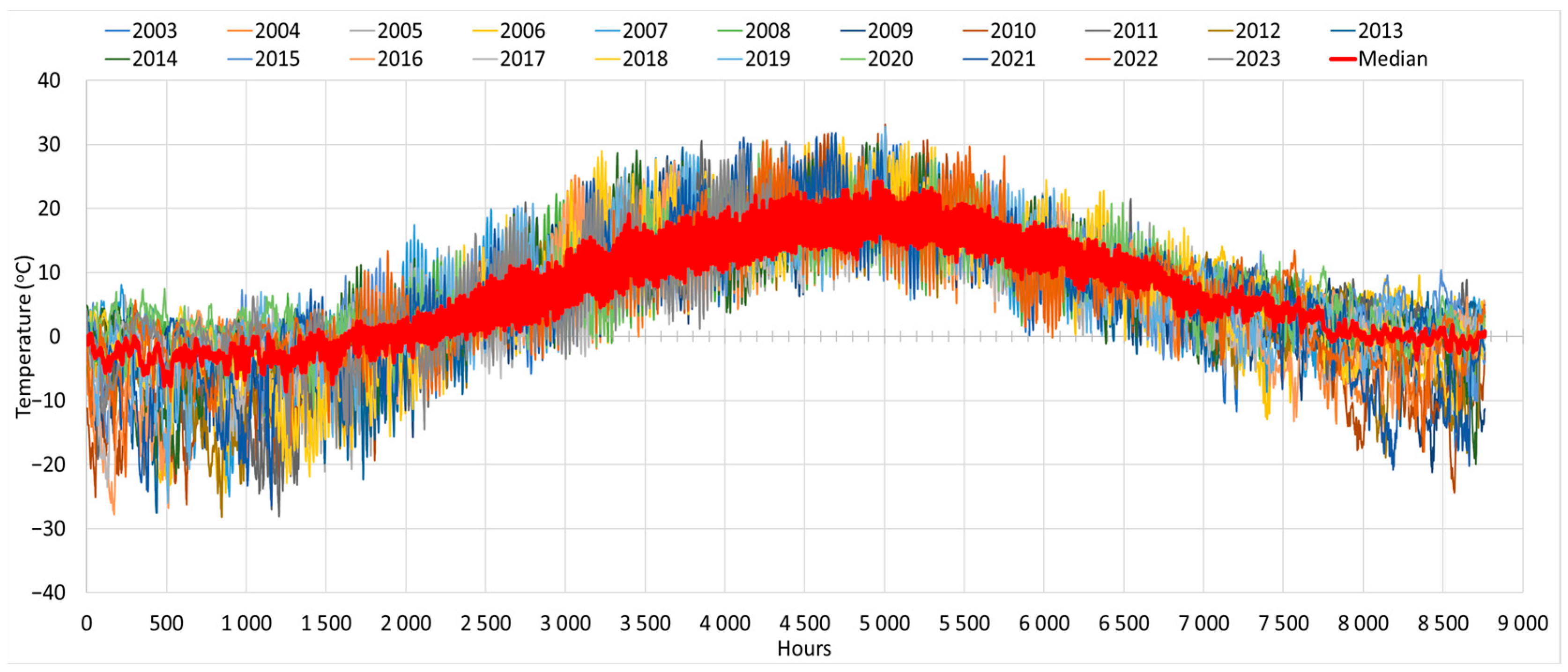
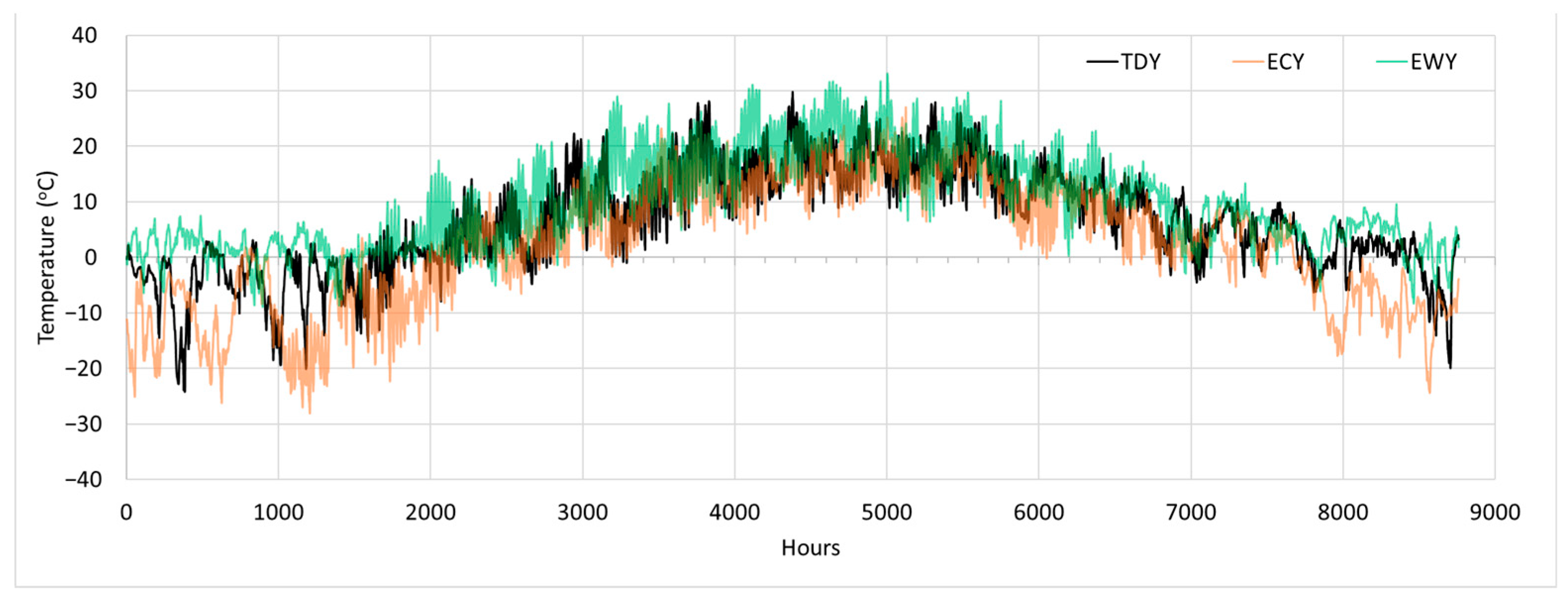
2.4. Weather: Typical and Extreme Conditions

Generally, in the building studies, typical weather conditions and typical weather datasets, such as typical meteorological year (TMY), are used [57]. Since extreme weather events significantly impact the resilience of building and urban systems, they should be incorporated into the assessment. The TMY assists in energy calculations; however, there are certain limitations. Hong et al. [58] conducted a study by using TMY and the actual metrological year for long-term assessment of building performance and found that energy savings and peak demand can be significantly different.

In this regard, three different sets of one-year weather data are used according to a method proposed by Nik [57], representing three separate years: a year with typical weather conditions (which is called typical downscaled year TDY in [57]), extreme cold year (ECY) and extreme warm year (EWY). In the original approach, these three weather datasets are synthesized considering a 30-year period; however, in this work, a 20-year period (2003–2023) is used due to the presence of some incomplete years. The measured weather data of Helsinki from the Finnish Meteorological Institute are employed to synthesize the weather data for [43] (1) typical downscaled year (TDY), the typical conditions; (2) ECY, representing the coldest conditions; and (3) EWY, representing the warmest conditions.

TDY is synthesized similarly to TMY but with the difference of weighting only the ambient temperature when selecting 12 typical meteorological months (TMMs). They are then concatenated in order to produce a weather file that is for 1 year. Moreover, the selection is based on the hourly ambient temperature. The synthesized weather data are generated for the ambient temperature, wind speed, humidity, wind direction, and solar radiation to include important climate data for simulation. The monthly quantile distributions of the outdoor temperature are calculated for all the years and for each year separately. The year with a distribution similar to those of all years is selected as the typical year (for that month). By repeating the procedure for all months, 12 typical months are recognized, shaping a typical year. The same steps are used to produce the ECY and EWY datasets. The years that have the maximum and minimum temperatures are chosen as the years representing the extreme temperatures.

Such synthesized data do not account for climatic uncertainties and represent an image for the considered time. The TDY, ECY, and EWY are based on the hourly outdoor temperature, and the other climatic parameters are not considered.

Uncertainties in future climate datasets affect each parameter differently. For example, few scenarios may exhibit a 20% variance in mean temperature and a 10% variance in wind data. For regional climate models (RCM) data, it is not feasible to track these differences and assign the correct weight factor. The TDY, EWY, and ECY climate data are generated to consider and represent different climate scenarios and to reduce the computation time. Otherwise, more simulations are needed to represent different performances of the buildings using 20 years of weather data. The application of using the representative weather datasets by Nik [57] has been validated for various types of analysis, including building energy simulations [59], assessment of urban energy systems [60], urban and micro-climate studies [61], as well as hygrothermal simulations [62].

Synthesized Weather Datasets: TDY, EWY and ECY

The hourly ambient temperatures, based on the measurements from 2003–2023, are shown in Figure 2 (in multi-color lines) as the reference. The red line represents the hourly average values derived from historical data. These average values are then compared to the measured data for each year. It is observed that while the trend remains similar across datasets, the hourly average data appear to be dampened.

The TDY, ECY, and EWY are shown in Figure 3. The highest probability is represented by TDY. The ECY represents the lower bound of the 20-year graph, and the EWY represents the upper bound.

Figure 4 demonstrates the hourly ambient temperature distribution between the historical data (20 years) and the TDY, EWY, and ECY in the Helsinki region. The red dotted line presents the historical data from 2003–2023. The ambient temperature in TDY (blue line) has a distribution similar to that of the historical data. The extreme ambient temperature distribution (yellow and grey lines) is also shown. Cold weather conditions (below 0 °C) are evident from the historical data for Finland. In this study, typical and extreme climate scenarios are considered to represent the building’s energy and resilience performance in various representative real conditions that may occur.

3. Energy Resilience: Technical and Economic Calculation Methods for Parametric Analysis

The energy resilience framework and indicators are defined in Section 3.1. In the parametric study, different renewable energy capacities, climate scenarios, and building types are used to compare the energy resilience performance of the buildings in Nordic conditions. These design variables for the parametric study are discussed in Section 3.2. Finally, the costing method used to calculate the costs for each simulation is also described, in Section 3.3.

3.1. Energy Resilience Framework and Indicator Calculations

To calculate the resilience performance of both the old and new buildings, various indicators are calculated. Figure 5 illustrates the multi-phased curve and behavior of the building during disruptive events such as blackouts and grid loss. Different performance phases are observable in Figure 5, with a similar approach proposed for building resilience in warm climatic conditions [27]. The curve depicted in Figure 5 is adjusted for winter’s climatic conditions. Phase I, labeled as “before the disruptive event”, Phase II as “during the disruptive event”, Phase III as “after the disruptive event”, and Phase IV as “after recovery from the disruptive event”, define and visually represent the building’s energy resilience. The behavior of the curve depends on the impact and duration of the power outage, the type of building envelope, and the energy system design (e.g., PV, storage, etc.).

In Figure 5, different thresholds can be observed. These are used to define the resilience metrics [35]. The following are explanations of the thresholds shown in Figure 5.

• P_ST represents the indoor set point temperature (i.e., 21.5 °C) [49].
• P_RT represents the robustness threshold. If the performance is below this point, then the building is not robust. The recommended value is 18 °C for health reasons [63].
• Robustness period (RP) give the length of time that the building remains robust after the power is cut.
• P_HT gives the habitability threshold for the occupants. Below this point, a building is unable to provide a minimum living environment for its occupants. Here, 15 °C is utilized as the threshold for habitability.
• P_min represents the minimum indoor temperature the building reaches during the power outage.
• Recovery speed (RS) gives the speed at which the building reaches the target indoor set point (21.5 °C) after the availability of power supply is restored.

Table 3. Energy resilience calculation metrics and indicators for performance analysis.

Indicator	Equation
Robustness threshold duration (RT)	t1 − t0
Collapse speed (CS)	(PST − PRT) + (PRT − Pmin)/t2 − t0
Impact of failure (IoF)	(PST − PRT) + (PRT − Pmin)
Recovery speed (RS)	(PST − PRT) + (PRT − Pmin)/t3 − t2

presents the metric calculations that are used to calculate the energy resilience performance.

• Robustness threshold duration (RT) = This represents the duration that the building’s indoor temperature can be maintained above the robustness threshold (P_RT). A higher value means the building is better prepared to face the disruptive event (power outage).
• Collapse speed (CS) = This represents the swiftness at which the building’s indoor temperature and performance drop from the set point to the habitability threshold P_HT. Lower value is better.
• Impact of failure (IoF) = This represents the power outage impact on the building’s performance. It presents the minimum performance of the building reached during the power outage. A smaller value means the building can absorb the disruptive event better and adapt.
• Recovery speed (RS) = This represents the speed at which the building’s indoor temperature reaches the target point after the availability of the power supply is restored.

The degree of disruption is also proposed as part of the resilience framework [64]. Equation (1) gives the degree of disruption (DoD):

$$\mathrm{DoD}={\displaystyle \frac{{Parameter}_{disruption}-{Parameter}_{reference}}{{Parameter}_{reference}}}\times {\displaystyle \frac{{Time}_{disruption}}{{Time}_{reference}}},$$

(1)

Equation (1) calculates the severity and impact on the performance of the building due to the power outage. Severity refers to the decrease or increase in the indoor temperature during the disruptive event defined as Parameter_disruption. Parameter_reference refers to the reference indoor set point temperature. The time duration is the ratio of the Time_disruption, i.e., t₂ − t₀ (duration of the disruptive event) in Figure 5, and Time_reference (i.e., the total observation time of the system). Time_reference = 31 h, and Parameter_reference is the indoor temperature, i.e., 21.5 °C [35]. All the aforementioned indicators of the resilience framework can be utilized to categorize the building’s performance based on its resilience performance. Colors can be used to rate the performance. The color red can denote the ‘worst’ performance, while green can indicate the ‘best’ performance. Other shades can represent performance levels between these two extremes.

3.2. Parametric Study

To analyze the behavior of both the old and new buildings in respect of energy resilience and onsite energy generation performance under typical, extremely cold, and warm climatic conditions, various design variables are utilized. The sizes of the PV and battery, building types, and season are varied to analyze the impact of typical and extreme climate change on energy generation and its impact on energy resilience performance.

Table 4. Input values for the case studies 1a, 1b, 1c (for old building), and 2a, 2b, 2c (for new building) in TDY, EWY, and ECY climate scenarios and during winter and spring seasons.

Building Type	Case Number	Climate Scenarios	Design Variables for Parametric Study		Tested Representative Seasons	Simulation Options
			Photovoltaic Panel’s Area Variable Values (m2)	Battery Capacity Variable Values (kWh)
Old building (Case 1)	1a	TDY	0	0, 44, 89, 133	Winter, spring	8
	1a	TDY	50	0, 44, 89, 133	Winter, spring	8
	1a	TDY	75	0, 44, 89, 133	Winter, spring	8
	1a	TDY	100	0, 44, 89, 133	Winter, spring	8
	1b	EWY	0	0, 44, 89, 133	Winter, spring	8
	1b	EWY	50	0, 44, 89, 133	Winter, spring	8
	1b	EWY	75	0, 44, 89, 133	Winter, spring	8
	1b	EWY	100	0, 44, 89, 133	Winter, spring	8
	1c	ECY	0	0, 44, 89, 133	Winter, spring	8
	1c	ECY	50	0, 44, 89, 133	Winter, spring	8
	1c	ECY	75	0, 44, 89, 133	Winter, spring	8
	1c	ECY	100	0, 44, 89, 133	Winter, spring	8
New building (Case 2)	2a	TDY	0	0, 44, 89, 133	Winter, spring	8
	2a	TDY	50	0, 44, 89, 133	Winter, spring	8
	2a	TDY	75	0, 44, 89, 133	Winter, spring	8
	2a	TDY	100	0, 44, 89, 133	Winter, spring	8
	2b	EWY	0	0, 44, 89, 133	Winter, spring	8
	2b	EWY	50	0, 44, 89, 133	Winter, spring	8
	2b	EWY	75	0, 44, 89, 133	Winter, spring	8
	2b	EWY	100	0, 44, 89, 133	Winter, spring	8
	2c	ECY	0	0, 44, 89, 133	Winter, spring	8
	2c	ECY	50	0, 44, 89, 133	Winter, spring	8
	2c	ECY	75	0, 44, 89, 133	Winter, spring	8
	2c	ECY	100	0, 44, 89, 133	Winter, spring	8

presents Case 1 for the old building and Case 2 for the new building, each with TDY, ECY, and EWY scenarios, and with varying PV and battery sizes. The total simulation cases are 96 for each building type and, in total, 192 simulations for both old and new building types.

The area of the PV is assumed to be 0 (no PV) to the maximum area of 100 m². The maximum area is assumed to cover all the building’s roof area, i.e., 100 m². The battery capacity is assumed to be 0 (no battery) to the maximum capacity of 133 kWh. The capacities of the battery are assumed to be the size of the available electric vehicle battery sizes [65]; also, these sizes are used in the earlier study [66]. This is assumed because old electric vehicle batteries can be reused for building applications. In each step, the sizes of PV and battery are doubled separately for the parametric study, until the maximum sizes as shown in Table 4. The scenarios without PV and battery are ‘passive’ resilience performance (reference), and those with PV and battery integration are ‘active’ resilience performance of the simulated buildings.

3.3. Cost Calculations

In this study, the total cost is calculated to estimate the investment and annual operational costs (maintenance and replacement costs) of the proposed energy system to improve energy resilience performance. The energy and disposal costs are not included. The PV and battery costs are described in

Table 5. The energy system components’ costs.

Cost Component	PV	Battery	Reference
Investment cost	124 €/m2	600 €/kWh	[67,68]
Operational and maintenance cost	1.5% of the investment cost	1.5% of the investment cost	[67,68]
Duration	25 years	12.5 years	[67,68]
Replacement cost	Included in the maintenance cost	200 €/kWh	[67,68]

.

The total cost includes the investment cost and the operation and maintenance costs. The future annual costs are estimated using the annual discount factors. The total cost is calculated using Equation (2) [67,68]:

Total cost = Investment cost + (operational and maintenance + replacement costs) ∗ df,

(2)

where investment cost includes the PV and battery initial cost. The operational and maintenance costs include the operations, maintenance, and replacement costs. The ‘df’ is the discount factor that is calculated using Equation (3) [67,68]:

$$df={\displaystyle \frac{1}{a}}(1-{\displaystyle \frac{1}{{(1+a)}^T}}),$$

(3)

where ‘df’ is the discount factor, and ‘a’ is the interest rate, which is assumed to be 3% [68]. The operation time ‘T’ is assumed to be 25 years. The replacement cost discount factor is calculated using Equation (4) [67,68]:

$$replacement factor={\displaystyle \frac{1}{{(1+a)}^{Tr}}},$$

(4)

The battery requires replacement during its lifetime. The replacement time ‘Tr’ is 12.5 years [68].

4. Results and Discussion

The simulated cases and parametric study results are presented in this Section. Section 4.1 presents different heating demands, Section 4.2 presents the techno-economic energy resilience performance of the old building (cases 1a, 1b, and 1c), and Section 4.3 presents the techno-economic performance of the new building (cases 2a, 2b and 2c).

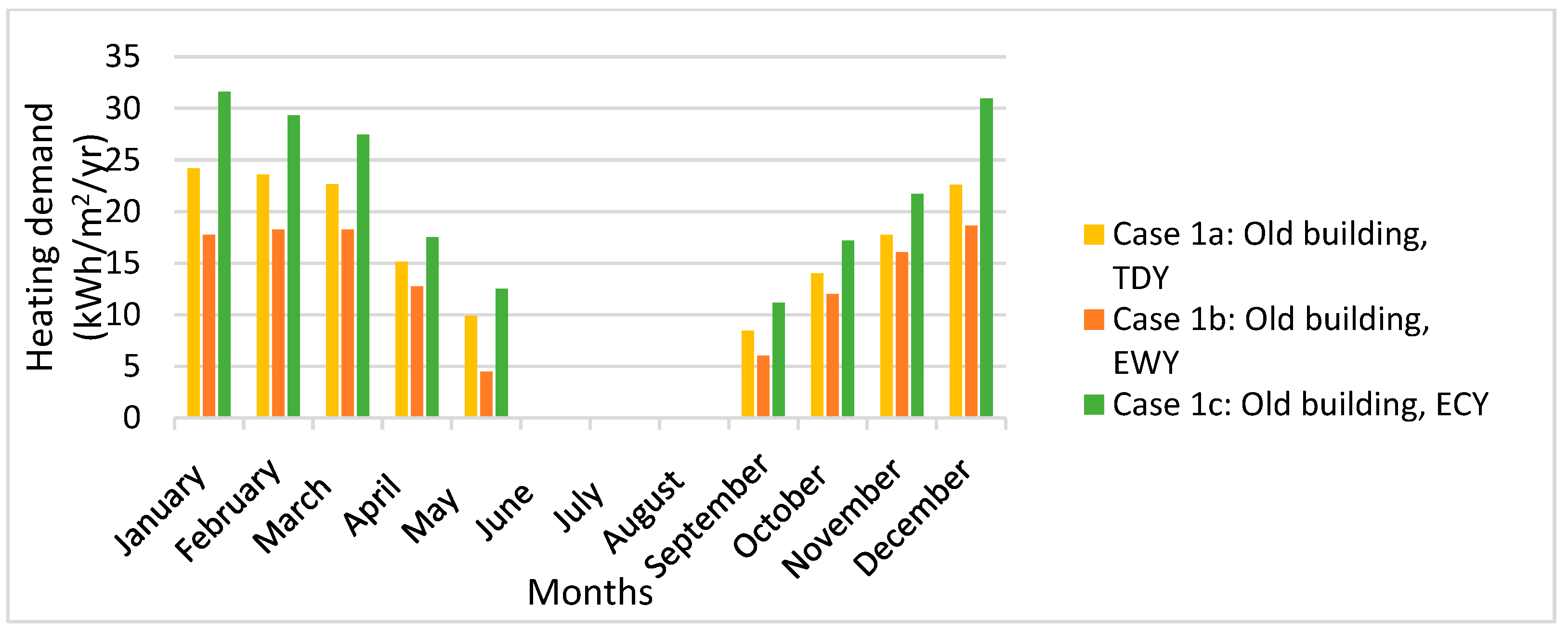
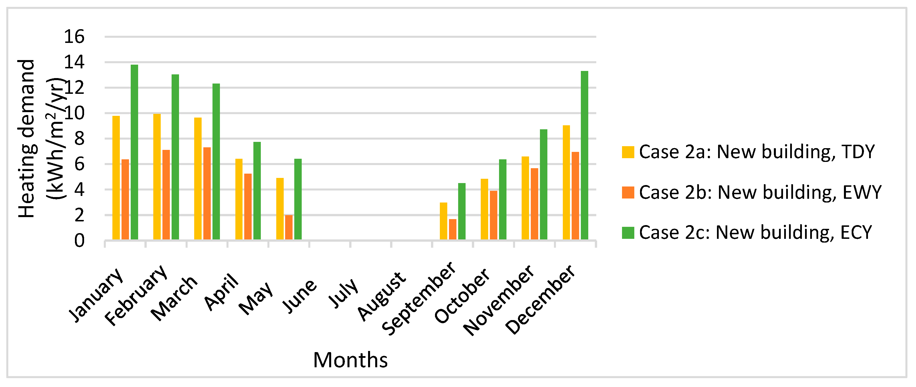
4.1. Old and New Building Heating Demands in TDY, EWY and ECY Climate Scenarios

The yearly performance is depicted in

Table 6. Climate scenarios and the annual old (case 1a, 1b, 1c) and new (case 2a, 2b, 2c) building performances.

	Climate Scenarios, Corresponding Heating Demand
Heating Demand Parameters, Old Building	TDY (1a)	EWY (1b)	ECY (1c)
Old building heating demand (kWh/m2/yr)	158.33	124.42	199.47
Difference in the heating demand from TDY (kWh/m2/yr)	-	−33.91	41.14
Relative difference in the demand from TDY (%)	-	21.5%	26%
	Climate Scenarios, Corresponding Heating Demand
Heating Demand Parameters, New Building	TDY (2a)	EWY (2b)	ECY (2c)
New building heating demand (kWh/m2/yr)	64.06	46.12	86.08
Difference in the demand from TDY (kWh/m2/yr)	-	−17.94	22.02
Relative difference in the demand from TDY (%)	-	28%	34.3%

. It is observed that in the EWY scenario, the heating demand decreased, as compared to the TDY. On the other hand, Table 6 shows that in the ECY scenario, the heating demand increased, compared to the TDY. It is also found that the new building has an overall lower heating demand compared to the old building. This could be attributed to the better insulation and efficient design of the new building that resulted in lower losses of heat energy from the building.

Figure 6 shows that for the same building, in the same location, variation in climate can cause big differences in monthly heating demand. This distribution is important to be presented, as climate can vary drastically during every month. The yellow bar represents the typical monthly heating demand of the old building during TDY. The green bar shows the heating demand of the old building during the ECY scenario, resulting in a larger heating demand compared to TDY. Conversely, the opposite happens under EWY climate conditions, as depicted by the orange bar.

Figure 7 illustrates the typical monthly heating demand of the new building for TDY, EWY, and ECY climate scenarios. Compared to the old building (Figure 6), it is found that the new building has a lower overall heating demand for each month.

The integration of Figure 3 (TDY, EWY, and ECY climate scenarios) with the old and new building simulation models provided the heating demands. Figure 6 (old building) and Figure 7 (new building) provide each building’s heating demand profiles under extreme and typical climate scenarios with acceptable accuracy and representation. TDY covers the typical conditions and the corresponding building heating demand. EWY covers the upper bound and the corresponding building heating demand. ECY covers that lower bound and the corresponding building heating demand. A similar method has been carried out in [57]. In the next section, an hourly scale parametric study is carried out to present the two buildings’ performances under TDY, ECY, and EWY climate scenarios and their energy resilience performances.

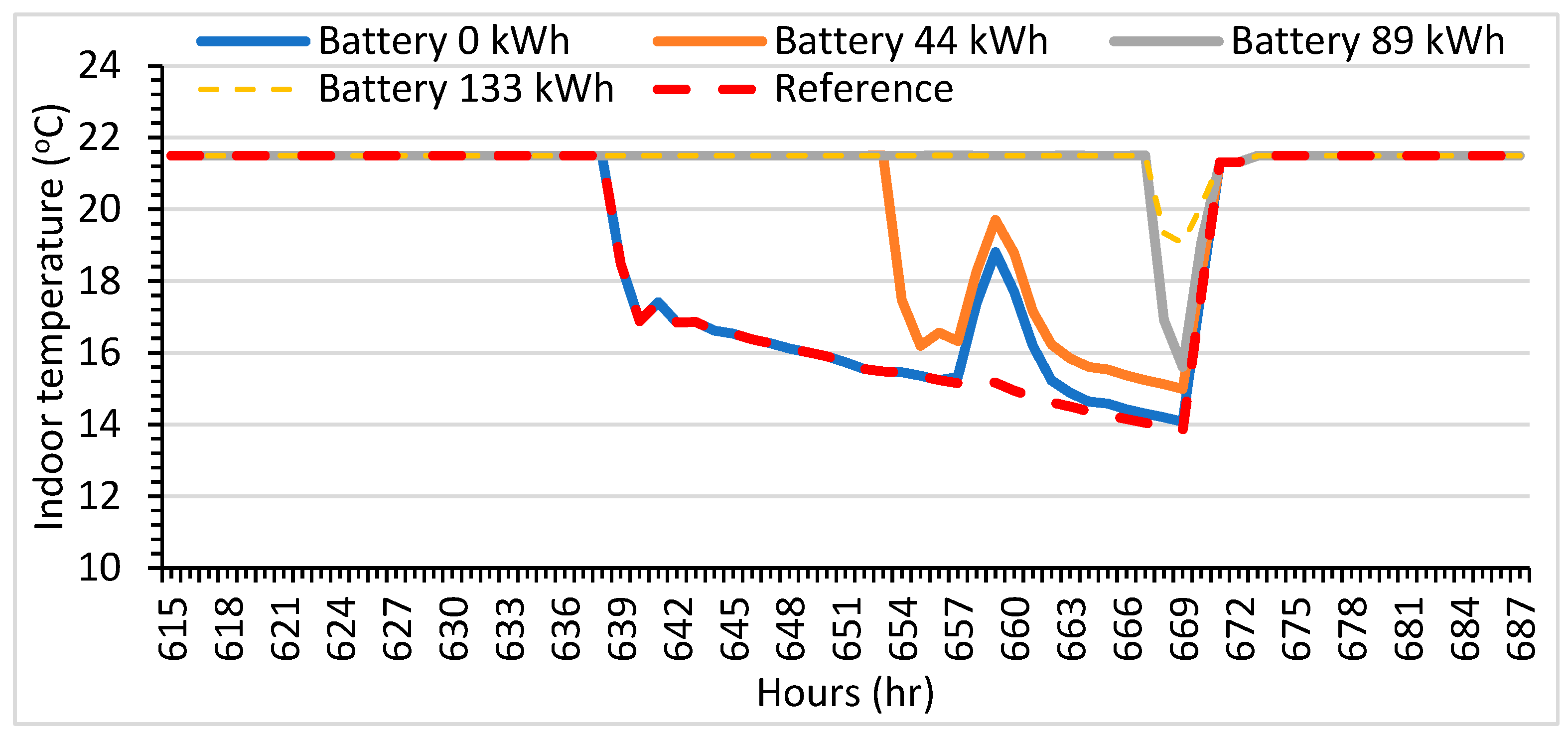
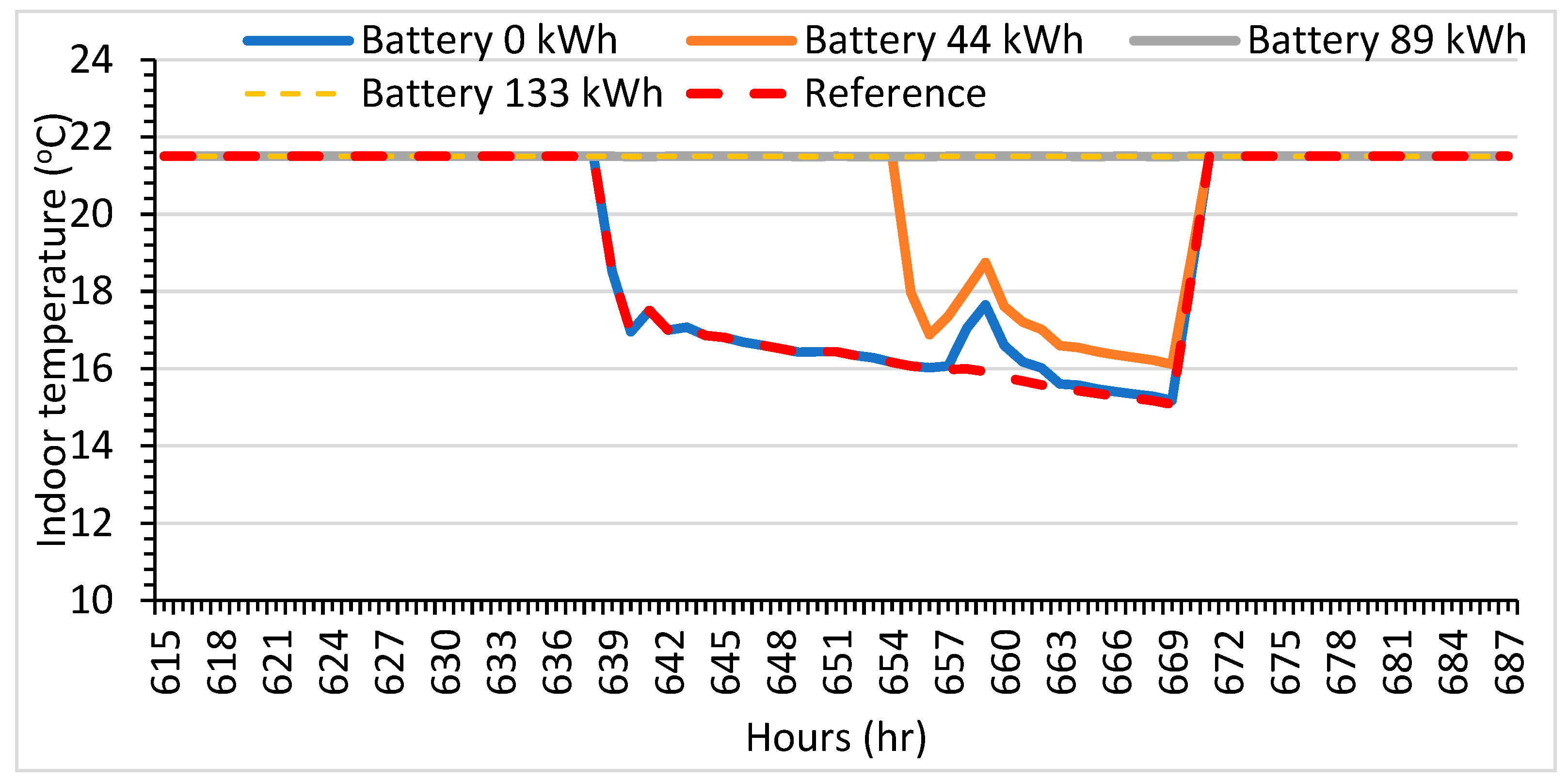
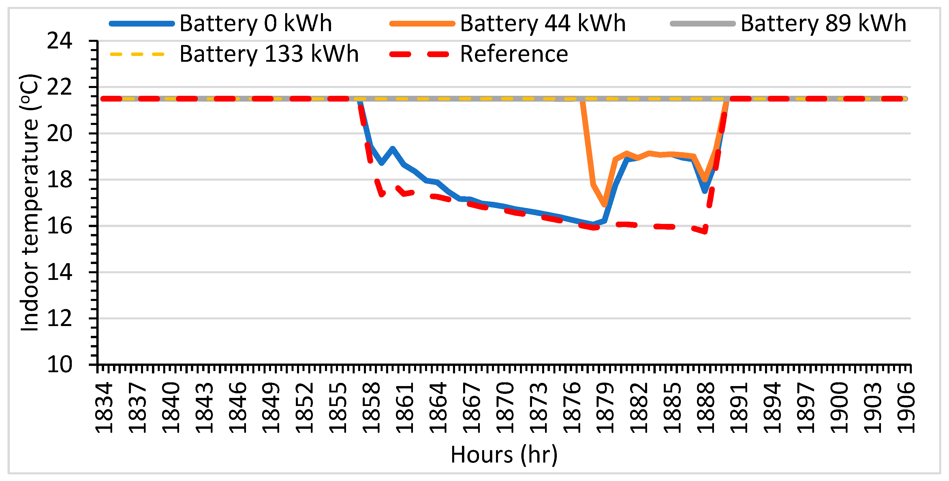
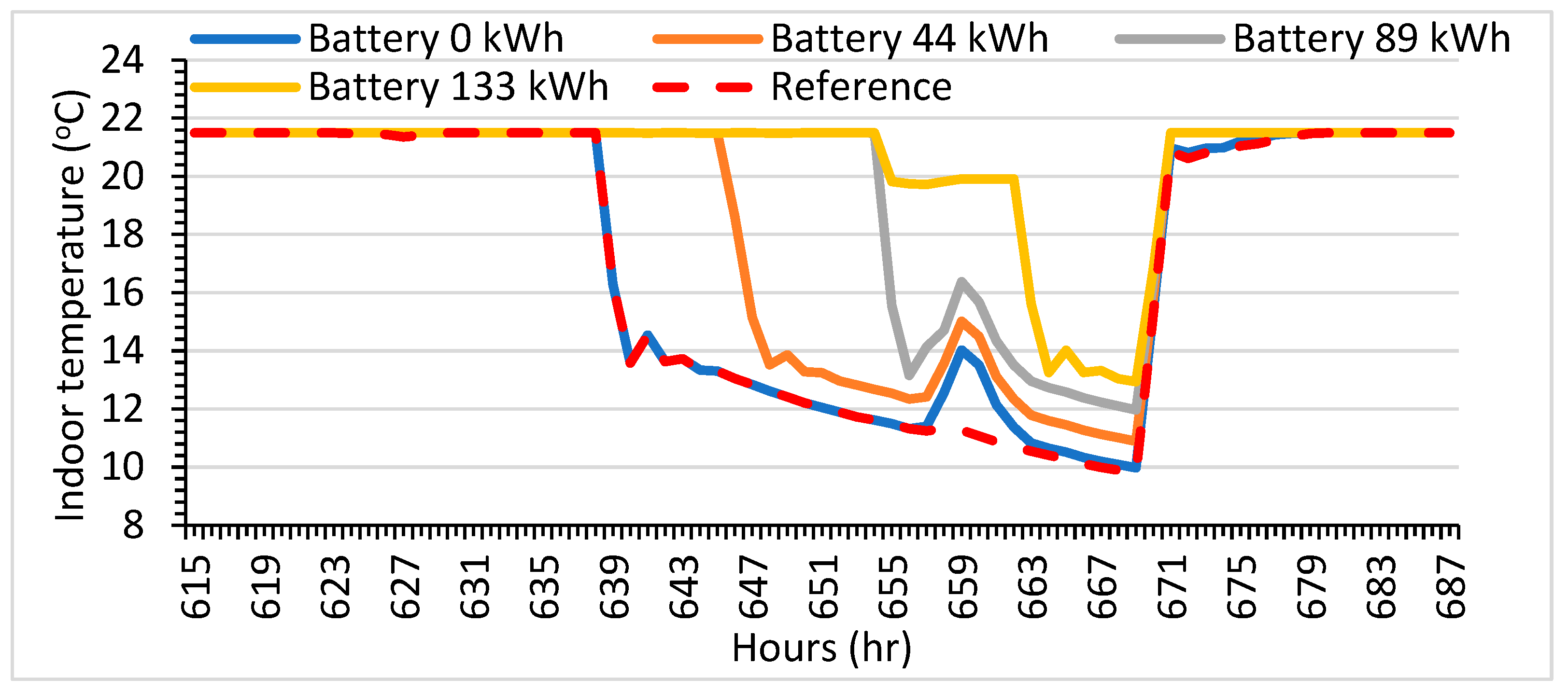
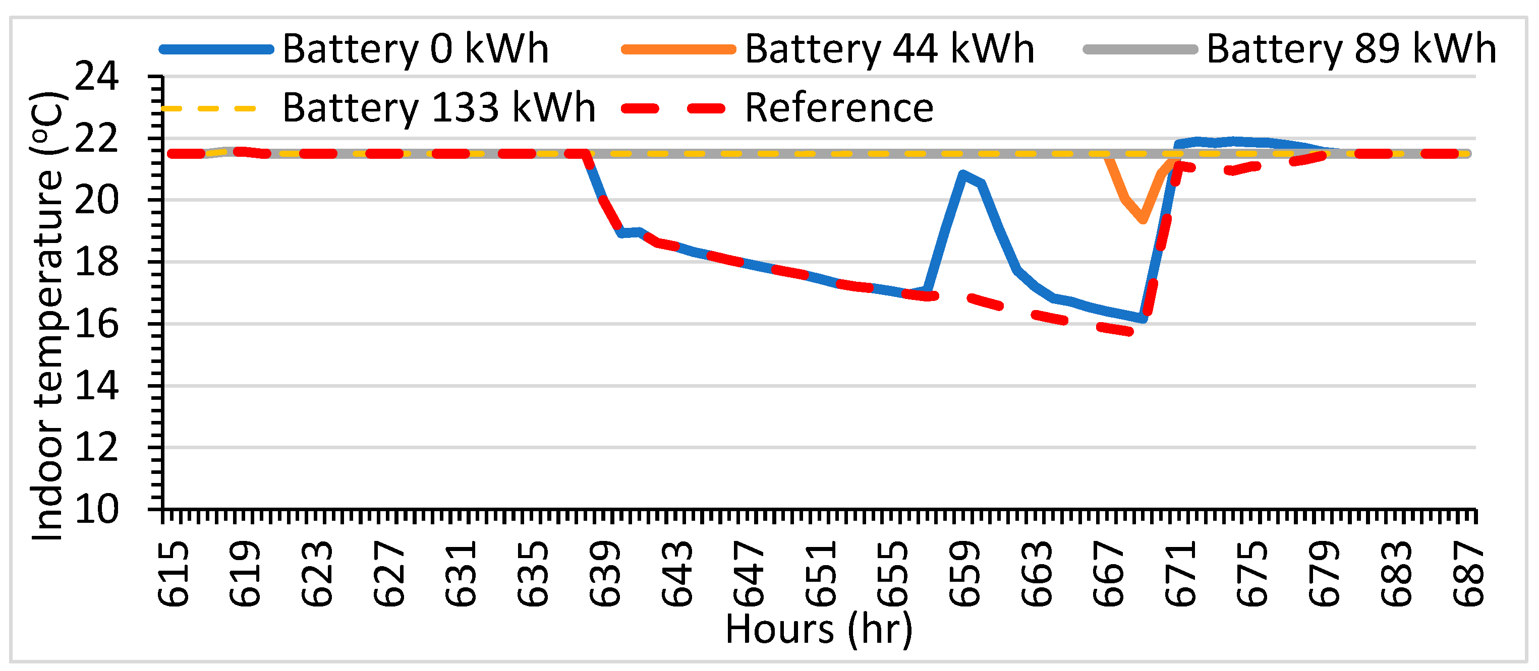
4.2. Energy Resilience in Old Building (Case 1)

The energy resilience performance of the old building in TDY (case 1a), EWY (case 1b), and ECY (case 1c) climate scenarios is presented during the winter and spring seasons.

4.2.1. Case 1a, Old Building: TDY

The energy resilience performance of the old building in TDY (case 1a) is presented during the winter and spring seasons.

Case 1a: Winter Season (TDY)

To examine the performance during the winter season (case 1a), a yearly simulation is carried out, and the hours selected for assessment range from 615 h to 687 h as a representative period for winter. The power outage duration of 31 h (winters) is selected based on the earlier studies carried out and literature review findings in [35,48,49,69]. This selection is made considering the reduced availability of solar radiation and an average ambient temperature of around −10 °C to −15 °C, reflecting the harsh conditions in the south of Finland. The power outage starts at 639 h and extends until 670 h, with a duration of 31 h, during which no electricity is available. The same simulation and power outage hours are applied consistently across all subsequent cases during the winter season (cases 1b and 1c). This approach is undertaken to assess the resilience performance of the old building under blackout conditions, both with and without PV systems and batteries. Figure 8 (red dotted line) illustrates that in the absence of PV and battery (the reference case), utilizing only the thermal mass (passive resilience), the indoor air temperature decreases from 21.5 °C to 18 °C within 2 h, reaching the robustness threshold. As the power outage persists, the habitability threshold is not met, dropping to 15 °C after 20 h. With indoor temperatures falling below 15 °C, the building demonstrates a lack of thermal resilience. The overall degree of disruption (DoD) is approximately 0.357, indicating a significant disruption to the energy resilience performance (DoD = 0 indicates the best resilience performance). The impact of failure (IoF) is 7.7 °C, collapse speed (CS) is 0.25 °C/h, and recovery speed (RS) is 1.91 °C/h.

The addition of energy storage such as batteries could compensate for the non-availability of grid power and solar energy. Hence, including batteries in the study is essential to analyze potential improvements in the energy resilience performance of the building.

When the same building (case 1a) is integrated with varying battery capacities and PV (100 m²), it is observed that the old building’s energy resilience performance changed during the grid outage. The blue line (Figure 8) indicates that with maximum PV capacity alone, the robustness threshold period is 2 h, and the habitability threshold of 15 °C is reached 23 h after crossing the robustness threshold. The overall degree of disruption can be classified in terms of energy resilience as 0.33, which is slightly high. Overall, the building’s energy resilience performance improves when integrated with PV.

The yellow dotted line (Figure 8) indicates that with maximum PV area and battery capacity, the robustness threshold duration improves to 30 h, and habitability conditions are consistently met, ensuring the temperature does not drop below 15 °C throughout the power outage period. This demonstrates improvement over the case where only thermal mass (passive method) is used for resilience (Figure 8, red dotted line) and also over the case where PV serves as the sole energy source (Figure 8, blue line). This indicates that the impact of the power outage is significantly reduced with the addition of a battery. Other indicators such as IoF, CS, RS, and costs are presented in (

Table A1. Parametric study, energy resilience performance analysis, and costs for case 1a in TDY (winter) climate scenario with varying PV and battery capacity.

PV Area, m2	0				50				75				100
Battery Capacity, kWh	0	44	89	133	0	44	89	133	0	44	89	133	0	44	89	133
Robustness duration (RT), hour	2.00	2.00	2.00	2.00	2.00	16.00	24.00	24.00	2.00	17.00	31.00	31.00	2.00	17.00	31.00	31.00
Impact of failure (IoF), °C	7.669	7.669	7.669	7.669	7.541	6.615	6.212	6.212	7.482	6.557	5.886	2.446	7.424	6.506	5.886	2.443
Collapse speed (CS), °C/h	0.247	0.247	0.247	0.247	0.243	0.213	0.200	0.200	0.241	0.212	0.190	0.079	0.239	0.217	0.190	0.079
Recovery speed (RS), °C/h	1.917	1.917	1.917	1.917	1.885	1.654	1.553	1.553	1.871	1.639	1.471	0.611	1.856	1.627	1.471	0.611
Degree of disruption (DoD)	0.357	0.357	0.357	0.357	0.351	0.308	0.289	0.289	0.348	0.305	0.274	0.114	0.334	0.293	0.274	0.114
PV cost (€)	0	0	0	0	6838	6838	6838	6838	9851	9851	9851	9851	12,864	12,864	12,864	12,864
Battery cost (€)	0	39,377	79,649	119,027	0	39,377	79,649	119,027	0	39,377	79,649	119,027	0	39,377	79,649	119,027

Colors grading variations: Red is the ‘worst’ performing and green is the ‘best’ performing cases.

) in Appendix A. Tables in Appendix A present the key performance indicator values for all the simulation results, and then these values are arranged in a color grading system. This is done to identify the energy resilience performance for each case and provides the optimal points and their corresponding design variables among all the simulated scenarios. The concept of color grading is introduced in the tables in Appendix A as an innovative approach to assess and rate the building’s energy resilience performance for all the following simulated cases. The color grading spectrum ranges from red to orange, yellow, and green (with various shades). The tables in Appendix A also show the corresponding costs to represent the cost associated with each combination of solutions. These costs can be used to provide the techno-economic optimal solutions.

The CS (in Table A1) is reduced with battery and PV, indicating that both PV and battery can minimize and delay the decline in indoor temperature. The RS is lower because the IoF is low with the battery, thus requiring minimal energy at a slow rate to return the indoor temperature to the set point of 21.5 °C after the grid is restored. This slow recovery rate is important, as it reduces sudden peaks and impacts on the grid, especially during grid restoration. With battery and PV integration in the old building, the overall DoD can be classified in terms of energy resilience as 0.114, which is lower compared to cases without PV and with PV alone. DoD can be used as a factor to compare and rate the buildings in terms of their energy resilience performance. The building can be classified as more resilient compared to cases with thermal mass only and with PV alone.

It is noted that scenarios lacking photovoltaic (PV) panels and batteries are represented in the red color grade, categorizing their performance as ‘worst’ (as depicted in Table A1). Conversely, it is observed that scenarios incorporating PV panels (100 m²) and batteries (133 kWh) are represented in the green color grade, denoting their performance as ‘best’ (in Table A1). Based on the energy resilience definition framework and utilizing the color grading system presented in Table A1, it is recommended that a PV area of 75 m2 (9851 €) and a battery capacity of 133 kWh (119,027 €) represent an optimal point. Increasing the PV area beyond this point does not lead to improved performance, thus enabling potential cost savings.

Case 1a: Spring Season (TDY)

Similarly to the winter season, spring season is shown to compare the building’s behavior and resilience performance between winter and spring seasons. This is to show and represent two different seasons and their impact on the building’s resilience performance and also as an extension to the earlier studies [35,48,49,69]. In Finland, the spring season also requires heating of the buildings. Yearly simulation is carried out, and the hours selected for assessment range from 1834 h to 1906 h as a representative period for spring. The duration of the power outage is the same as for the winter season [35,48,49,69]. The power outage is assumed to occur between 1858 h to 1889 h, with a duration of 31 h when grid power is unavailable. This selection is made when solar radiation is available, and the average temperature ranges from 0 °C to −5 °C in southern Finland. The same simulation and power outage hours are considered in all the following cases during the spring season in cases 1b and 1c.

It is observed in Figure 9 (red dotted line) that without PV and battery, while utilizing only the thermal mass of the building (passive resilience), the indoor temperature decreases from 21.5 °C to 18 °C within 4 h, resulting in a robustness threshold duration of 4 h. As the power outage persists, the indoor temperature remains above 15 °C (above the habitability threshold). Therefore, the building can be deemed thermally resilient during the spring season. The IoF, CS, and RS indicators are presented in

Table A2. Parametric study, energy resilience performance analysis, and costs for case 1a in TDY (spring) climate scenario with varying PV and battery capacity.

PV Area, m2	0				50				75				100
Battery Capacity, kWh	0	44	89	133	0	44	89	133	0	44	89	133	0	44	89	133
Robustness duration (RT), hour	4.00	4.00	4.00	4.00	8.00	21.00	31.00	31.00	9.00	21.00	31.00	31.00	9.00	21.00	31.00	31.00
Impact of failure (IoF), °C	5.963	5.963	5.963	5.963	5.774	5.129	0.013	0.013	5.717	5.130	0.013	0.013	5.697	5.130	0.013	0.013
Collapse speed (CS), °C/h	0.284	0.284	0.284	0.284	0.275	0.244	0.001	0.001	0.272	0.244	0.001	0.001	0.247	0.217	0.190	0.079
Recovery speed (RS), °C/h	0.497	0.497	0.497	0.497	0.481	0.513	0.001	0.001	0.476	0.513	0.001	0.001	0.475	0.513	0.001	0.001
Degree of disruption (DoD)	0.188	0.188	0.188	0.188	0.182	0.162	0.000	0.000	0.180	0.162	0.000	0.000	0.180	0.162	0.000	0.000
PV cost (€)	0	0	0	0	6838	6838	6838	6838	9851	9851	9851	9851	12,864	12,864	12,864	12,864
Battery cost (€)	0	39,377	79,649	119,027	0	39,377	79,649	119,027	0	39,377	79,649	119,027	0	39,377	79,649	119,027

Colors grading variations: Red is the ‘worst’ performing and green is the ‘best’ performing cases.

and are better than those for the winter season. The overall degree of disruption (DoD) is approximately 0.188. Compared to the winter season for case 1a without PV and battery (Figure 8), it is observed that during the spring season, the old building in the TDY climate scenario can provide better resilience. This is attributed to the availability of solar energy and fewer losses, as the ambient temperature is slightly higher during spring.

The blue line (Figure 9) shows that with a maximum PV area (100 m²) and no battery, the robustness period extends to 9 h, and the habitability threshold is maintained during the power outage as the indoor temperature remains above 15 °C. Table A2 presents IoF, CS, and RS indicators, which are better than those observed during the winter season. The yellow dotted line indicates that with the maximum PV area and battery capacity, the robustness duration improves to 31 h, and the building maintains robustness throughout the entire power outage. This demonstrates that the impact of the power outage on the building is significantly reduced with the presence of a battery, as evidenced by the reduction in IoF and CS and the increase in RS (Table A2). The integration of PV and battery supports resilience during the recovery phase. With the integration of battery and PV, the overall degree of disruption can be classified in terms of energy resilience as 0, which is low compared to the cases without PV and with PV alone. The building remains unaffected by the disruption, and occupants do not experience the effects of power loss. Grey line and yellow dotted line overlap each other.

Based on the color grading in Table A2, it can be recommended that the optimal point is achieved with a PV area of 50 m² and a battery capacity of 89 kWh. Additional design variable capacities are unnecessary, as further performance enhancement is not significant. A comparison with the winter season, as depicted in Table A1, reveals improved performance during the spring season in Table A2. This improvement is evident from the differences in color grading between the two tables, where the optimal point and corresponding color grade shift to green for a smaller PV area and battery capacity. Specifically, during the spring season, the optimal point is observed with a PV area of 50 m² (6838 €) and a battery capacity of 89 kWh (79,649 €), whereas during winter, it is observed with a PV area of 75 m² (9851 €) and a battery capacity of 133 kWh (119,027 €).

4.2.2. Case 1b, Old Building: EWY

The energy resilience performance of the old building in EWY (case 1b) is presented during the winter and spring seasons.

Case 1b: Winter Season (EWY)

To analyze the performance of the old building during the winter season in the EWY scenario, the hours selected for simulation and power outage are identical to those in case 1a (winter season). As depicted in Figure 10 by the red dotted line, it is observed that utilizing the thermal mass of the building alone (passive resilience), results in a reduction in indoor air temperature from 21.5 °C to 18 °C within 3 h (until reaching the robustness threshold). Despite the continuation of the power outage, the building maintains a temperature above the habitability threshold of 15 °C. The IoF is 6.42 °C, CS is 0.2 °C/h, and RS is 3.212 °C/h. The overall degree of disruption (DoD) is approximately 0.299, indicating a high level of disruption. Compared to case 1a in TDY in the winter season (in Figure 8), the same building remains above the habitability threshold of 15 °C in case 1b, EWY (Figure 10, red dotted line). Furthermore, in other parameters such as IoF, CS, RS, and DoD, the building in this case performs better. This improvement is attributed to warmer climatic conditions and lower losses in the EWY climatic scenario.

The blue line shown in Figure 10 illustrates that without the battery and with maximum PV capacity, the robustness period is 3 h, and the building remains habitable (with indoor temperature above 15 °C). The overall DoD is 0.294. The yellow dotted line demonstrates that with the maximum PV area and battery capacity, the robustness duration improves to 31 h, and habitability conditions (15 °C or above) are consistently met throughout the entire power outage period. This indicates an enhancement compared to case 1b, where only thermal mass is utilized for resilience (red dotted line), and also in the case where only PV is used. The IoF, CS, and RS show improvement compared to the case without PV, as shown in

Table A3. Parametric study, energy resilience performance analysis, and costs for case 1b in EWY (winter) climate scenario with varying PV and battery capacity.

PV Area, m2	0				50				75				100
Battery Capacity, kWh	0	44	89	133	0	44	89	133	0	44	89	133	0	44	89	133
Robustness duration (RT), hour	3.00	3.00	3.00	3.00	3.00	17.00	30.00	31.00	3.00	17.00	31.00	31.00	3.00	17.00	31.00	31.00
Impact of failure (IoF), °C	6.424	6.424	6.424	6.424	6.370	5.438	3.704	1.976	6.345	5.413	0.012	0.012	6.320	5.389	0.012	0.012
Collapse speed (CS), °C/h	0.207	0.207	0.207	0.207	0.205	0.175	0.119	0.064	0.205	0.175	0.000	0.000	0.204	0.174	0.000	0.000
Recovery speed (RS), °C/h	3.212	3.212	3.212	3.212	3.185	2.719	1.852	0.988	2.115	2.707	0.006	0.006	2.107	2.694	0.006	0.006
Degree of disruption (DoD)	0.299	0.299	0.299	0.299	0.296	0.253	0.172	0.092	0.295	0.252	0.001	0.001	0.294	0.251	0.001	0.001
PV cost (€)	0	0	0	0	6838	6838	6838	6838	9851	9851	9851	9851	12,864	12,864	12,864	12,864
Battery cost (€)	0	39,377	79,649	119,027	0	39,377	79,649	119,027	0	39,377	79,649	119,027	0	39,377	79,649	119,027

Colors grading variations: Red is the ‘worst’ performing and green is the ‘best’ performing cases.

. The overall degree of disruption can be classified in terms of energy resilience as 0 (best). Grey line and yellow dotted line overlap each other.

Table A3 shows the key performance indicators of all 16 simulation scenarios with varying PV and battery capacities, for the old building in the EWY climate scenario during winters. Based on the color grading in Table A3, it is recommended that the optimal configuration include a PV area of 50 m² and a battery capacity of 89 kWh. A comparison with case 1a (TDY) during winter in Section Case 1a: Winter Season (TDY) reveals a reduction in PV area from 75 m² to 50 m² and a decrease in battery capacity from 133 kWh to 89 kWh in the EWY scenario. Hence, it is evident that with a warmer climatic scenario, both PV area and battery capacity can be decreased. This means that the cost of the PV and the battery is 30.5% and 33% lower, respectively, in EWY compared to the same building in TDY climate conditions.

Case 1b: Spring Season (EWY)

In Figure 11 (red dotted line), it is observed that by utilizing the thermal mass of the building solely (passive resilience), the indoor temperature decreases from 21.5 °C to 18 °C over a period of 5 h. As the power outage continues, the indoor temperature remains above 15 °C, which is the habitability threshold. The overall degree of disruption (DoD) is approximately 0.180. When compared to case 1a in TDY in the spring season (in Figure 9), the same building performed better in terms of IoF, CS, and RS. This improvement can be attributed to warmer climatic conditions and lower losses in the EWY climatic scenario. Furthermore, it is evident that the DoD during spring in case 1b is lower compared to that of case 1a.

The blue line in Figure 11 illustrates that with maximum PV area alone, the robustness threshold period reaches 10 h, and the building remains habitable and resilient as the indoor temperature stays above 15 °C. The overall DoD is 0.172. Additionally, the yellow dotted line indicates that with the maximum PV area and battery capacity, the robustness duration extends to 31 h, and habitability conditions (above 15 °C) are consistently maintained throughout the entire power outage period. This shows an improvement over case 1b where only thermal mass is used for resilience (Figure 11, red dotted line), as well as over the case where PV is used as the only source of energy (Figure 11, blue line). The IoF, CS, and RS are detailed in

Table A4. Parametric study, energy resilience performance analysis, and costs for case 1b in EWY (spring) climate scenario with varying PV and battery capacity.

PV Area, m2	0				50				75				100
Battery Capacity, kWh	0	44	89	133	0	44	89	133	0	44	89	133	0	44	89	133
Robustness duration (RT), hour	5.00	5.00	5.00	5.00	9.00	23.00	31.00	31.00	10.00	23.00	31.00	31.00	10.00	23.00	31.00	31.00
Impact of failure (IoF), °C	5.749	5.749	5.749	5.749	5.508	4.635	0.007	0.007	5.473	4.609	0.007	0.007	5.445	4.583	0.007	0.007
Collapse speed (CS), °C/h	0.185	0.185	0.185	0.185	0.178	0.150	0.000	0.000	0.177	0.149	0.000	0.000	0.176	0.148	0.000	0.000
Recovery speed (RS), °C/h	2.875	2.875	2.875	2.875	2.754	2.317	0.004	0.004	2.737	2.304	0.002	0.002	2.722	2.292	0.002	0.002
Degree of disruption (DoD)	0.180	0.180	0.180	0.180	0.174	0.153	0.000	0.000	0.172	0.152	0.000	0.000	0.172	0.151	0.000	0.000
PV cost (€)	0	0	0	0	6838	6838	6838	6838	9851	9851	9851	9851	12,864	12,864	12,864	12,864
Battery cost (€)	0	39,377	79,649	119,027	0	39,377	79,649	119,027	0	39,377	79,649	119,027	0	39,377	79,649	119,027

Colors grading variations: Red is the ‘worst’ performing and green is the ‘best’ performing cases.

. The overall DoD can be classified as 0 (best). Grey line and yellow dotted line overlap each other.

Table A4 shows the key performance indicators of all 16 simulation scenarios with varying PV and battery capacities. Based on the energy resilience definition and using the color grading in Table A4, it can be recommended that a PV area of 50 m² and a battery capacity of 89 kWh represent an optimal point. However, with a 44 kWh battery capacity, the building still exhibited good resilience. When compared to case 1b (TDY) during spring in Section Case 1a: Spring Season (TDY), it is observed that the PV area in EWY remained at 50 m² and the battery capacity decreased from 89 kWh to 44 kWh. Therefore, in a warmer climatic scenario, both the PV area and battery capacity can be reduced. This means that the cost of the PV is the same and that of the battery is 50% lower in EWY compared to the same building in TDY climate conditions.

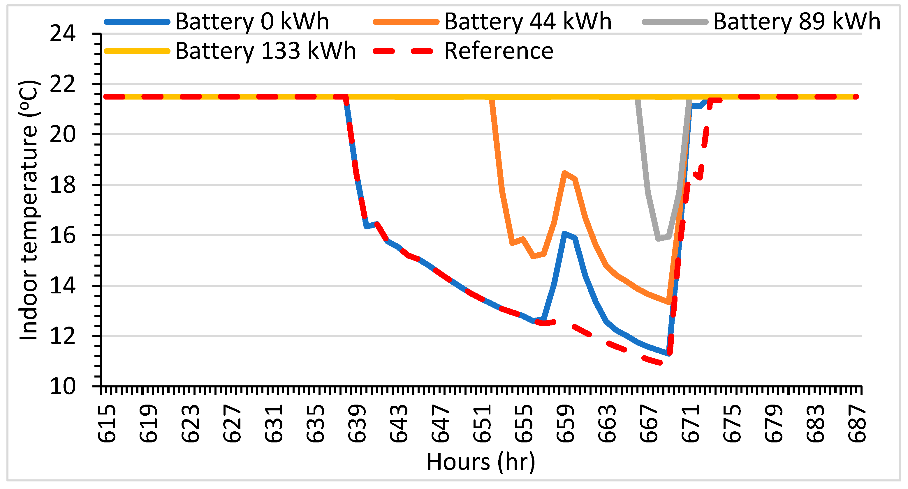
4.2.3. Case 1c, Old Building: ECY

The energy resilience performance of the old building in ECY (case 1c) is presented during the winter and spring seasons.

Case 1c: Winter Season (ECY)

In Figure 12 (red dotted line), it is observed that utilizing the thermal mass of the building alone (passive resilience) resulted in a reduction in indoor air temperature from 21.5 °C to 18 °C within 1 h. As the power outage continues, it is noted that the indoor temperature dropped to the habitability threshold of 15 °C within 1 h after surpassing the robustness threshold. Once the indoor temperature falls below 15 °C, the building ceases to be thermally resilient. The IoF is 11.72 °C, CS is 0.387 °C/h, and RS is 0.977 °C/h. The overall DoD is 0.545, indicating a high level of disruption.

Compared to case 1a in TDY and case 1b in EWY in the winter season, the same building exhibits a worse robustness threshold in case 1c in ECY during winter (in Figure 12). Furthermore, the building struggles to maintain the habitability threshold of 15 °C for an extended duration (in Figure 12). Other indicators such as IoF, CS, and RS demonstrate that the building performs worse in case 1c during winter compared to the same building in cases 1a and 1b during winter. This can be attributed to colder climatic conditions and higher losses in the ECY climatic scenario. Additionally, it is evident that the DoD in case 1c during winter is higher compared to the DoD in cases 1a and 1b during winter. Therefore, it can be concluded that the same building may face worse conditions and perform poorly in terms of energy resilience if the climate is colder than the typical year.

The blue line (Figure 12) illustrates that with maximum PV capacity alone, the robustness period is 1 h, and the building remains inhabitable as the indoor temperature drops below 15 °C within an hour. The overall DoD is 0.536. The yellow line demonstrates that with maximum PV area and battery capacity, the robustness duration improves to 26 h. This indicates an improvement over case 1c, where only thermal mass is utilized for resilience (Figure 12, red dotted line), and also over the case where PV is solely used as an energy source (blue line). The DoD is 0.398. Hence, energy resilience performance can be enhanced in the ECY climatic scenario. However, compared to case 1a (Section Case 1a: Winter Season (TDY)) and case 1b (Section Case 1b: Winter Season (EWY)), the performance in case 1c is the worst.

Table A5. Parametric study, energy resilience performance analysis, and costs for case 1c in ECY (winter) climate scenario with varying PV and battery capacity.

PV Area, m2	0				50				75				100
Battery Capacity, kWh	0	44	89	133	0	44	89	133	0	44	89	133	0	44	89	133
Robustness duration (RT), hour	1.00	1.00	1.00	1.00	1.00	8.00	17.00	17.00	1.00	9.00	17.00	24.00	1.00	10.00	18.00	26.00
Impact of failure (IoF), °C	11.723	11.723	11.723	11.723	11.618	10.706	9.624	9.624	11.570	10.650	9.576	8.739	11.523	10.608	9.528	8.553
Collapse speed (CS), °C/h	0.378	0.378	0.378	0.378	0.375	0.345	0.310	0.310	0.373	0.344	0.309	0.282	0.372	0.342	0.307	0.276
Recovery speed (RS), °C/h	0.977	0.977	0.977	0.977	1.056	5.353	4.812	4.812	1.157	5.325	4.788	4.370	1.152	5.304	4.764	4.277
Degree of disruption (DoD)	0.545	0.545	0.545	0.545	0.540	0.498	0.448	0.448	0.538	0.495	0.445	0.406	0.536	0.493	0.443	0.398
PV cost (€)	0	0	0	0	6838	6838	6838	6838	9851	9851	9851	9851	12,864	12,864	12,864	12,864
Battery cost (€)	0	39,377	79,649	119,027	0	39,377	79,649	119,027	0	39,377	79,649	119,027	0	39,377	79,649	119,027

Colors grading variations: Red is the ‘worst’ performing and green is the ‘best’ performing cases.

shows the key performance indicators of all 16 simulation scenarios with varying PV and battery capacities. Based on the color grading in Table A5, it can be recommended that the optimal point is reached with a PV area of 100 m² and a battery capacity of 133 kWh. In comparison to case 1a (TDY) during winter in Section Case 1a: Winter Season (TDY), the PV area in ECY increased from 75 m² to 100 m², and the battery capacity increased from 89 kWh to 133 kWh to attain the optimal point and green color code. However, the robustness threshold is reached at 26 h with maximum PV area and battery capacity. Therefore, in colder climatic scenarios, it may be necessary to increase the PV area and battery capacity. This means that the costs of the PV and the battery are 23.4% and 49.4% higher, respectively, in ECY compared to the same building in TDY climate conditions.

Case 1c: Spring Season (ECY)

It is observed in Figure 13 (red dotted line) that using the thermal mass of the building solely (passive resilience) resulted in a decrease in indoor temperature from 21.5 °C to 18 °C within 1 h. As the power outage persisted, the indoor temperature reached the habitability threshold of 15 °C after passing the robustness threshold, within 9 h. Comparatively, the building in case 1c is not resilient during the spring season, unlike in case 1a and case 1b. The overall DoD is approximately 0.372. Additionally, it is noticeable that the DoD in case 1c is higher for spring compared to case 1a and case 1b. Hence, DoD serves as a metric to communicate the performance and impact of the same building under different climatic conditions.

Figure 13 (blue line) illustrates that with maximum PV area only, the robustness period lasts for 7 h. As the power outage persists, the indoor temperature reaches the habitability threshold of 15 °C within 8 h after surpassing the robustness threshold. When the indoor temperature drops below 15 °C, the building loses its thermal resilience. The DoD is 0.233, with additional indicators presented in

Table A6. Parametric study, energy resilience performance analysis, and costs for case 1c in ECY (spring) climate scenario with varying PV and battery capacity.

PV Area, m2	0				50				75				100
Battery Capacity, kWh	0	44	89	133	0	44	89	133	0	44	89	133	0	44	89	133
Robustness duration (RT), hour	1.00	1.00	1.00	1.00	6.00	16.00	30.00	31.00	7.00	16.00	30.00	31.00	7.00	16.00	31.00	31.00
Impact of failure (IoF), °C	8.005	8.005	8.005	8.005	7.479	6.733	5.301	3.100	7.424	6.708	5.128	3.050	7.408	6.716	4.854	3.010
Collapse speed (CS), °C/h	0.381	0.381	0.381	0.381	0.356	0.321	0.252	0.098	0.354	0.319	0.244	0.098	0.353	0.320	0.231	0.098
Recovery speed (RS), °C/h	0.500	0.500	0.500	0.500	0.288	0.259	0.265	0.190	0.286	0.258	0.256	0.190	0.285	0.258	0.243	0.190
Degree of disruption (DoD)	0.372	0.372	0.372	0.372	0.236	0.212	0.167	0.141	0.234	0.211	0.162	0.141	0.233	0.212	0.153	0.141
PV cost (€)	0	0	0	0	6838	6838	6838	6838	9851	9851	9851	9851	12,864	12,864	12,864	12,864
Battery cost (€)	0	39,377	79,649	119,027	0	39,377	79,649	119,027	0	39,377	79,649	119,027	0	39,377	79,649	119,027

Colors grading variations: Red is the ‘worst’ performing and green is the ‘best’ performing cases.

.

The yellow dotted line indicates that with maximum PV area and battery capacity, the robustness duration extends to 31 h, and the habitability condition (above 15 °C) is consistently maintained throughout the power outage period. In ECY case 1c (during spring), the IoF and CS decrease, while the RS increases (Table A6). The DoD is 0.141, which is an improvement in ECY during spring.

Based on the definition of energy resilience and using the color grading in Table A6, it can be recommended that a PV area of 50 m² and a battery capacity of 133 kWh represent the optimal point. In comparison with the winter season in case 1c (Figure 12), both PV and battery capacities decreased to achieve optimal performance. Furthermore, a comparison with case 1a (TDY) during spring in Section Case 1a: Spring Season (TDY), indicates that the PV area in ECY remained constant at 50 m², while the battery capacity increased from 89 kWh to 133 kWh. This means that the cost of the PV is the same and that of the battery is 49.4% higher in ECY compared to the same building in TDY climate conditions.

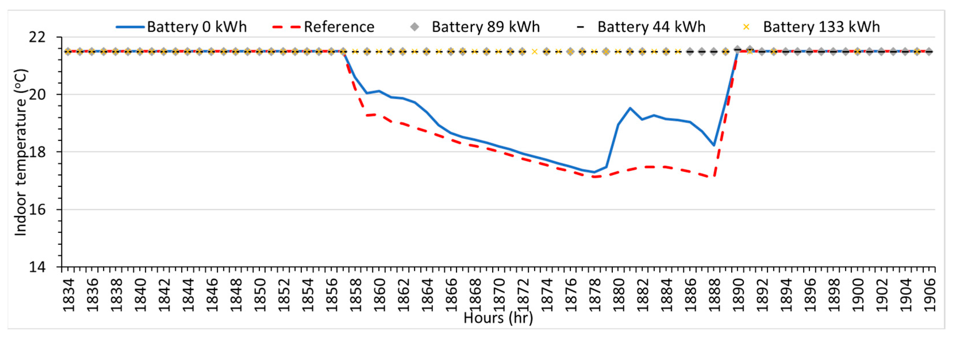
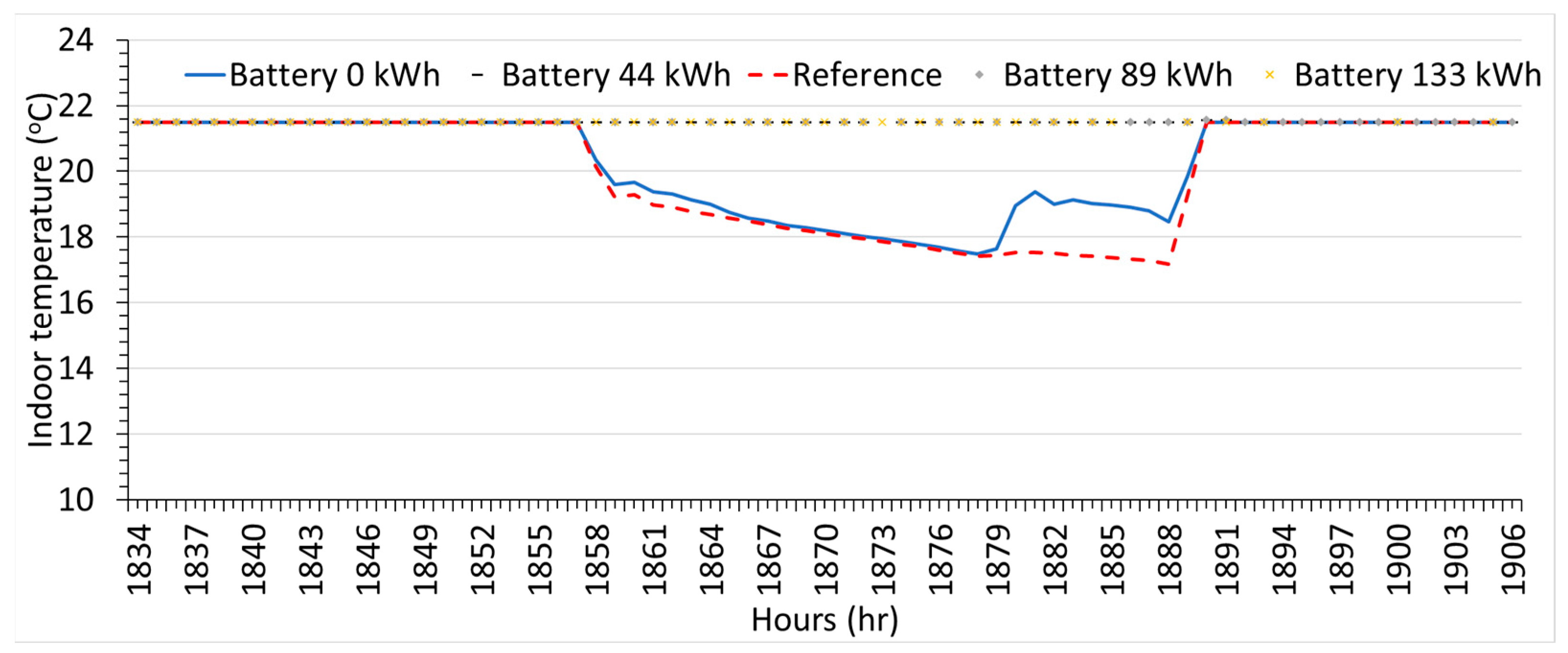
4.3. Energy Resilience in New Building (Case 2)

The energy resilience performance of the new building in TDY (case 2a), EWY (case 2b), and ECY (case 2c) climate scenarios is presented during the winter and spring seasons.

4.3.1. Case 2a, New Building: TDY

The energy resilience performance of the new building in TDY (case 2a) is presented during the winter and spring seasons.

Case 2a: Winter Season (TDY)

To study the performance of the new building during the winter season in cases 2a, 2b, and 2c, the hours selected for assessment and power outage are the same as those in Section 4.2. It is observed in Figure 14 (red dotted line) that without PV and battery (passive resilience), the indoor air temperature decreased from 21.5 °C to 18 °C in 10 h (until the robustness threshold). As the power outage persists, the building remains habitable and does not drop below the habitability threshold of 15 °C during the power outage. Compared to the old building, all indicators have improved (IoF = 5.582 °C, CS = 0.188 °C/h, and RS = 0.529 °C/h, as shown in

Table A7. Parametric study, energy resilience performance analysis, and costs for case 2a in TDY (winter) climate scenario with varying PV and battery capacity.

PV Area, m2	0				50				75				100
Battery Capacity, kWh	0	44	89	133	0	44	89	133	0	44	89	133	0	44	89	133
Robustness duration (RT), hour	10.00	10.00	10.00	10.00	10.00	31.00	31.00	31.00	10.00	31.00	31.00	31.00	10.00	31.00	31.00	31.00
Impact of failure (IoF), °C	5.824	5.824	5.824	5.824	5.534	2.120	0.002	0.002	5.403	2.120	0.002	0.002	5.332	2.120	0.002	0.002
Collapse speed (CS), °C/h	0.188	0.188	0.188	0.188	0.179	0.068	0.000	0.000	0.174	0.068	0.000	0.000	0.172	0.068	0.000	0.000
Recovery speed (RS), °C/h	0.529	0.529	0.529	0.529	2.767	1.060	0.001	0.001	2.701	1.060	0.001	0.001	2.666	1.060	0.001	0.001
Degree of disruption (DoD)	0.271	0.271	0.271	0.271	0.257	0.099	0.000	0.000	0.251	0.099	0.000	0.000	0.248	0.099	0.000	0.000
PV cost (€)	0	0	0	0	6838	6838	6838	6838	9851	9851	9851	9851	12,864	12,864	12,864	12,864
Battery cost (€)	0	39,377	79,649	119,027	0	39,377	79,649	119,027	0	39,377	79,649	119,027	0	39,377	79,649	119,027

Colors grading variations: Red is the ‘worst’ performing and green is the ‘best’ performing cases.

). The DoD improved to 0.271. The blue line (Figure 14) indicates that with maximum PV capacity only, the robustness period is 10 h, and the building remains habitable. The DoD is 0.248 (which is better). The yellow dotted line in Figure 14 shows that with the maximum PV area and battery capacity, the robustness duration improved to 31 h and the habitability conditions were consistently met. The DoD is 0. The IoF, CS, and RS are shown in Table A7. Table A7 shows the key performance indicators of all 16 simulation scenarios with varying PV and battery capacities. Grey line and yellow dotted line overlap each other.

As discussed earlier, color grading is used to represent the performance of the building in terms of energy resilience. In comparison to the old building in Section Case 1a: Winter Season (TDY), the optimal point for the new building in the same TDY climatic scenario can be achieved with a smaller PV area and battery capacity. Therefore, based on the energy resilience framework and utilizing the color grading in Table A7, it is recommended that the optimal point is a PV area of 50 m² (6838 €) and a battery capacity of 44 kWh (39,377 €).

Case 2a: Spring Season (TDY)

Similarly to the winter season, the performance of the new building during the spring season is also evaluated under TDY climatic conditions. The same assessment hours and power outage are considered as in case 1a during the spring season. It is observed in Figure 15 (red dotted line) that without PV and battery (passive resilience), the indoor air temperature decreases from 21.5 °C to 18 °C in 15 h (up to the robustness threshold). As the power outage persists, the building remains habitable and does not fall below the habitability threshold of 15 °C. In comparison to the old building discussed in Section Case 1a: Spring Season (TDY), all indicators such as IoF, CS, and RS have improved, as shown in

Table A8. Parametric study, energy resilience performance analysis, and costs for case 2a in TDY (spring) climate scenario with varying PV and battery capacity.

PV Area, m2	0				50				75				100
Battery Capacity, kWh	0	44	89	133	0	44	89	133	0	44	89	133	0	44	89	133
Robustness duration (RT), hour	15.00	15.00	15.00	15.00	16.00	31.00	31.00	31.00	16.00	31.00	31.00	31.00	16.00	31.00	31.00	31.00
Impact of failure (IoF), °C	4.425	4.425	4.425	4.425	4.208	0.001	0.001	0.001	4.208	0.001	0.001	0.001	4.208	0.001	0.001	0.001
Collapse speed (CS), °C/h	0.211	0.211	0.211	0.211	0.200	0.000	0.000	0.000	0.200	0.000	0.000	0.000	0.200	0.000	0.000	0.000
Recovery speed (RS), °C/h	0.369	0.369	0.369	0.369	0.351	0.001	0.001	0.001	0.351	0.001	0.001	0.001	0.351	0.001	0.001	0.001
Degree of disruption (DoD)	0.139	0.139	0.139	0.139	0.133	0.000	0.000	0.000	0.133	0.000	0.000	0.000	0.133	0.000	0.000	0.000
PV cost (€)	0	0	0	0	6838	6838	6838	6838	9851	9851	9851	9851	12,864	12,864	12,864	12,864
Battery cost (€)	0	39,377	79,649	119,027	0	39,377	79,649	119,027	0	39,377	79,649	119,027	0	39,377	79,649	119,027

Colors grading variations: Red is the ‘worst’ performing and green is the ‘best’ performing cases.

. The DoD improved to 0.139. Compared to the winter season (Figure 14), the new building during spring (in TDY climate) demonstrates better resilience.

The blue line (Figure 15) illustrates that with maximum PV capacity only, the robustness period is 16 h, and the habitability threshold is maintained, as the indoor temperature remains above 15 °C. The overall DoD is 0.133 when the old building is integrated with 100 m² PV (without the battery). The yellow (cross marked line) demonstrates that with the maximum PV area and battery capacity, the robustness duration improves to 31 h, and the building remains robust throughout the entire power outage. The overall DoD is classified as 0. Grey and black marks overlap yellow cross marked line.

Compared to the old building in Section Case 1a: Spring Season (TDY), the optimal point for the new building in the same TDY climatic scenario can be achieved with a smaller PV area and battery capacity. Therefore, based on the energy resilience framework and utilizing the color grading in Table A8, it can be recommended that an optimal point is a PV area of 50 m² (6838 €) and a battery capacity of 44 kWh (39,377 €). Table A8 shows the key performance indicators of all 16 simulation scenarios with varying PV and battery capacities.

4.3.2. Case 2b, New Building: EWY

The energy resilience performance of the new building in EWY (case 2b) is presented during the winter and spring seasons.

Case 2b: Winter Season (EWY)

In Figure 16(red dotted line), it is observed that without PV and battery, the indoor air temperature decreased from 21.5 °C to 18 °C in 15 h (until reaching the robustness threshold). Despite the ongoing power outage, the building remains habitable and does not drop below the habitability threshold of 15 °C. The old building barely maintains habitability in case 1b EWY winter season without PV. Compared to the old building in Section Case 1b: Winter Season (EWY), all indicators have improved (IoF = 4.784 °C, CS = 0.154 °C/h, and RS = 2.39 °C/h). The DoD has improved, reaching 0.223 compared to the old building.

The blue line in Figure 16 illustrates that with maximum PV capacity only, the robustness period extends to 16 h, and the building remains habitable. The DoD is 0.212 (an improvement) compared to the same case without PV (Figure 16, red dotted line). The yellow (cross marked line) indicates that with maximum PV area and battery capacity, the robustness duration improves to 31 h, and habitability conditions are consistently met. Overall, the new building’s performance surpasses that of the old building in Section Case 1b: Winter Season (EWY), in terms of the robustness threshold, as it has increased. The IoF and CS are also lower for the new building. Grey and black marks overlap yellow cross marked line.

Table A9. Parametric study, energy resilience performance analysis, and costs for case 2b in EWY (winter) climate scenario with varying PV and battery capacity.

PV Area, m2	0				50				75				100
Battery Capacity, kWh	0	44	89	133	0	44	89	133	0	44	89	133	0	44	89	133
Robustness duration (RT), hour	15.00	15.00	15.00	15.00	15.00	31.00	31.00	31.00	16.00	31.00	31.00	31.00	16.00	31.00	31.00	31.00
Impact of failure (IoF), °C	4.784	4.784	4.784	4.784	4.661	0.002	0.002	0.002	4.605	0.002	0.002	0.002	4.548	0.002	0.002	0.002
Collapse speed (CS), °C/h	0.154	0.154	0.154	0.154	0.150	0.000	0.000	0.000	0.149	0.000	0.000	0.000	0.147	0.000	0.000	0.000
Recovery speed (RS), °C/h	2.392	2.392	2.392	2.392	2.4	0.001	0.001	0.001	2.4	0.001	0.001	0.001	2.4	0.001	0.001	0.001
Degree of disruption (DoD)	0.223	0.223	0.223	0.223	0.217	0.000	0.000	0.000	0.214	0.000	0.000	0.000	0.212	0.000	0.000	0.000
PV cost (€)	0	0	0	0	6838	6838	6838	6838	9851	9851	9851	9851	12,864	12,864	12,864	12,864
Battery cost (€)	0	39,377	79,649	119,027	0	39,377	79,649	119,027	0	39,377	79,649	119,027	0	39,377	79,649	119,027

Colors grading variations: Red is the ‘worst’ performing and green is the ‘best’ performing cases.

is used to present the color grading and optimal points among all simulated scenarios in case 2b during winter. Utilizing the color grading in the table, it is recommended that a PV area of (6838 €) and a battery capacity of 44 kWh (39,377 €) represent an optimal point to achieve the energy resilient performance of the building.

Case 2b: Spring Season (EWY)

In Figure 17 (red dotted line), it is observed that without PV and battery, the indoor air temperature decreased from 21.5 °C to 18 °C in 18 h (up to the robustness threshold). The building remains habitable and does not fall below the habitability threshold of 15 °C. The Degree of Disruption (DoD) reached 0.136. The blue line in Figure 17 illustrates that with maximum PV capacity, the robustness period lasts 18 h, and the habitability threshold is maintained, as the indoor temperature stays above 15 °C. The IoF, RS, and CS are displayed in

Table A10. Parametric study, energy resilience performance analysis, and costs for case 2b in EWY (spring) climate scenario with varying PV and battery capacity.

PV Area, m2	0				50				75				100
Battery Capacity, kWh	0	44	89	133	0	44	89	133	0	44	89	133	0	44	89	133
Robustness duration (RT), hour	18.00	18.00	18.00	18.00	19.00	31.00	31.00	31.00	19.00	31.00	31.00	31.00	19.00	31.00	31.00	31.00
Impact of failure (IoF), °C	4.324	4.324	4.324	4.324	4.009	0.001	0.001	0.001	4.009	0.001	0.001	0.001	4.009	0.001	0.001	0.001
Collapse speed (CS), °C/h	0.206	0.206	0.206	0.206	0.191	0.000	0.000	0.000	0.191	0.000	0.000	0.000	0.191	0.000	0.000	0.000
Recovery speed (RS), °C/h	0.309	0.309	0.309	0.309	0.334	0.000	0.000	0.000	0.334	0.000	0.000	0.000	0.334	0.000	0.000	0.000
Degree of disruption (DoD)	0.136	0.136	0.136	0.136	0.126	0.000	0.000	0.000	0.126	0.000	0.000	0.000	0.126	0.000	0.000	0.000
PV cost (€)	0	0	0	0	6838	6838	6838	6838	9851	9851	9851	9851	12,864	12,864	12,864	12,864
Battery cost (€)	0	39,377	79,649	119,027	0	39,377	79,649	119,027	0	39,377	79,649	119,027	0	39,377	79,649	119,027

Colors grading variations: Red is the ‘worst’ performing and green is the ‘best’ performing cases.

. The DoD is 0.126. The yellow (cross marked line) indicates that with maximum PV area and battery capacity, the robustness duration improves to 31 h, and the building maintains robustness throughout the entire power outage. The IoF, CS, and RS are all 0, as shown in Table A10. The overall DoD can be classified as 0. Grey and black marks overlap yellow cross marked line.

In comparison to the old building mentioned in Section Case 1b: Spring Season (EWY), the optimal point for the new building in the EWY climatic scenario can be attained with a smaller battery capacity and a similar PV area. Based on the color grading in Table A10, the optimal point consists of a PV area of 50 m² and a battery capacity of 44 kWh. However, it is evident from Table A10 that even with a PV area of 50 m² and a battery capacity of 0 kWh, reasonable performance during a power outage can still be achieved. Therefore, with the new building, the cost of the energy system can be further reduced to ensure sufficient resilience. This means that the cost of the PV is 6838 € and that of the battery is 0 in this case.

4.3.3. Case 2c, New Building: ECY

The energy resilience performance of the new building in ECY (case 2c) is presented during the winter and spring seasons.

Case 2c: Winter Season (ECY)

In Figure 18 (red dotted line), it is observed that using the thermal mass of the building alone, the indoor air temperature decreased from 21.5 °C to 18 °C within 3 h (up to the robustness threshold). As the power outage continued, it was noted that the indoor temperature dropped to the habitability threshold of 15 °C within 5 h after surpassing the robustness threshold. In comparison to the old building in ECY case 1c (during winters) as discussed in Section Case 1c: Winter Season (ECY), the new building provided a longer duration of robustness threshold and habitability conditions without PV and battery. The IoF is 10.66 °C, CS is 0.334 °C/h, and RS is 1.77 °C/h (as indicated in

Table A11. Parametric study, energy resilience performance analysis, and costs for case 2c in ECY (winter) climate scenario with varying PV and battery capacity.

PV Area, m2	0				50				75				100
Battery Capacity, kWh	0	44	89	133	0	44	89	133	0	44	89	133	0	44	89	133
Robustness duration (RT), hour	3.00	3.00	3.00	3.00	3.00	14.00	29.00	30.00	3.00	15.00	29.00	31.00	3.00	15.00	29.00	31.00
Impact of failure (IoF), °C	10.660	10.660	10.660	10.660	10.418	8.375	5.636	5.654	10.307	8.265	5.636	0.021	10.197	8.155	5.636	0.021
Collapse speed (CS), °C/h	0.344	0.344	0.344	0.344	0.336	0.270	0.188	0.188	0.332	0.267	0.188	0.001	0.340	0.263	0.188	0.001
Recovery speed (RS), °C/h	1.777	1.777	1.777	1.777	1.736	2.094	2.818	2.827	2.577	2.755	2.818	0.010	2.039	2.718	2.818	0.010
Degree of disruption (DoD)	0.496	0.496	0.496	0.496	0.485	0.390	0.254	0.254	0.479	0.384	0.254	0.001	0.459	0.379	0.254	0.001
PV cost (€)	0	0	0	0	6838	6838	6838	6838	9851	9851	9851	9851	12,864	12,864	12,864	12,864
Battery cost (€)	0	39,377	79,649	119,027	0	39,377	79,649	119,027	0	39,377	79,649	119,027	0	39,377	79,649	119,027

Colors grading variations: Red is the ‘worst’ performing and green is the ‘best’ performing cases.

). The DoD reached 0.496 compared to the old building in Section Case 1c: Winter Season (ECY).

Compared to case 2a in TDY in the winter season and case 2b in EWY, the same building exhibited the worst robustness and habitability threshold in case 2c in ECY during winters. Furthermore, the new building failed to maintain 15 °C for an extended duration. The other KPIs such as IoF, CS, and RS showed that the building in the case 2c climatic scenario during winters performed worse compared to the same building in cases 2a and 2b during winters (Table A11). Moreover, it can be observed that the DoD in case 2c during winter is higher compared to the DoD in cases 2a and 2b during winter.

The blue line shows (Figure 18) that with maximum PV capacity, the robustness period is 3 h, and the building remains inhabitable after an hour but is thermally not resilient (as the indoor temperature drops below 15 °C within an hour). The overall DoD is 0.459. The yellow line illustrates that with maximum PV area and battery capacity, the robustness duration improves to 31 h. This demonstrates an enhancement within case 2c where PV is utilized as the only energy source. With the integration of battery and PV, the DoD improved from 0.496 (without PV and battery) to 0.

Based on the indicators and using the color grading in Table A11, the optimal point can be achieved using a PV area of 50 m² and a battery capacity of 89 kWh. When compared to the old building in Section Case 1c: Winter Season (ECY), it is observed that the PV area in case 2c ECY decreased from 100 m² to 50 m² and the battery capacity decreased from 133 kWh to 89 kWh to reach the optimal point and green color grade. This means that the costs of the PV and the battery are 46% and 33% lower, respectively, compared to the old building in ECY climate conditions.

Case 2c: Spring Season (ECY)

In Figure 19 (red dotted line), it is observed that without PV and battery, the indoor temperature decreased from 21.5 °C to 18 °C in 8 h. As the power outage continues, it is observed that the indoor temperature barely maintains the habitability threshold of 15 °C. Compared to case 1c (Section Case 1c: Spring Season (ECY)), the new building can maintain the habitability threshold and can be deemed resilient during the spring season in case 2c. Compared to the same building in case 2c in ECY during the spring season, case 2a and case 2b performed worse in terms of IoF, CS, and RS (

Table A12. Parametric study, energy resilience performance analysis, and costs for case 2c in ECY (spring) climate scenario with varying PV and battery capacity.

PV Area, m2	0				50				75				100
Battery Capacity, kWh	0	44	89	133	0	44	89	133	0	44	89	133	0	44	89	133
Robustness duration (RT), hour	8.00	8.00	8.00	8.00	8.00	31.00	31.00	31.00	8.00	31.00	31.00	31.00	9.00	31.00	31.00	31.00
Impact of failure (IoF), °C	6.094	6.094	6.094	6.094	5.512	0.001	0.001	0.001	5.507	0.001	0.001	0.001	5.502	0.001	0.001	0.001
Collapse speed (CS), °C/h	0.290	0.290	0.290	0.290	0.262	0.000	0.000	0.000	0.262	0.000	0.000	0.000	0.262	0.000	0.000	0.000
Recovery speed (RS), °C/h	0.508	0.508	0.508	0.508	0.551	0.000	0.000	0.000	0.551	0.000	0.000	0.000	0.611	0.000	0.000	0.000
Degree of disruption (DoD)	0.192	0.192	0.192	0.192	0.174	0.000	0.000	0.000	0.174	0.000	0.000	0.000	0.173	0.000	0.000	0.000
PV cost (€)	0	0	0	0	6838	6838	6838	6838	9851	9851	9851	9851	12,864	12,864	12,864	12,864
Battery cost (€)	0	39,377	79,649	119,027	0	39,377	79,649	119,027	0	39,377	79,649	119,027	0	39,377	79,649	119,027

Colors grading variations: Red is the ‘worst’ performing and green is the ‘best’ performing cases.

). This is attributed to colder climatic conditions and higher losses in the ECY climatic scenario. Furthermore, it can be observed that the DoD in case 2c is higher for spring compared to case 2a and case 2b in spring. The blue line (Figure 19) demonstrates that with maximum PV area only, the robustness period is 9 h. Additionally, the building remains habitable during the power outage, with an overall DoD of 0.173. The yellow (cross marked line) indicates that with maximum PV area and battery capacity, the robustness duration improves to 31 h, and habitability conditions (15 °C or above) are consistently met throughout the entire power outage period. Grey and black marks overlap yellow cross marked line.

Based on the energy resilience definition and using the color grading in Table A12, it can be recommended that the PV area of 50 m² and battery capacity of 89 kWh represent an optimal point. When compared to case 1c (ECY) during spring in Section Case 1c: Spring Season (ECY), it is observed that the PV area in case 2c (ECY) during spring remained close to 50 m² (6838 €); however, the battery capacity decreased to 44 kWh (39,377 €) to reach the optimal point and green color grade.

Based on the findings in Section 4.2 and Section 4.3, some of the points to be discussed are as follows:

• It has been found that during winters, both buildings perform worse compared to the spring season for all climatic scenarios (TDY, EWY, and ECY). Both the buildings in winter have a shorter duration of robustness and habitability thresholds compared to the spring season. Therefore, efforts are needed to improve the performance of the buildings during winter.
• The color rating system introduced in the study is based on the proposed energy resilience framework and key performance indicators. It is observed that usually the collapse speed is slower, and the recovery speed is faster in the spring season compared to the same building in winter. However, these two indicators depend on the impact of failure.
• Typically, during EWY, it has been found that the same building has a longer duration for the robustness and habitability threshold. On the contrary, during ECY, it has been found that the same building performs worse, as it has a shorter duration for the robustness and habitability thresholds. This can also be observed when using the proposed color grading system and DoD to rate the performance of the building.
• The new building performed better in terms of the robustness threshold, habitability threshold, and impact of failure. Moreover, the collapse speed and recovery speed are better for the new building.
• Table 7. Energy resilience performance analysis for case 1a and case 2a in TDY (winter) climate scenario with and without PV and battery.

  PV Area, m2	0				50				75				100
  Battery Capacity, kWh	0	44	89	133	0	44	89	133	0	44	89	133	0	44	89	133
  Case 1a (TDY) winters: Degree of disruption (DoD)	0.357	0.357	0.357	0.357	0.351	0.308	0.289	0.289	0.348	0.305	0.274	0.114	0.334	0.293	0.274	0.114
  Case 2a (TDY) winters: Degree of disruption (DoD)	0.271	0.271	0.271	0.271	0.257	0.099	0.000	0.000	0.251	0.099	0.000	0.000	0.248	0.099	0.000	0.000

  Colors grading variations: Red is the ‘worst’ performing and green is the ‘best’ performing cases.

  compares the combined DoD performances of the new and old buildings for the TDY climatic scenario, during winters. Most of the DoD for the new building has yellow and green colors, indicating good performance. On the other hand, the old building has orange and red colors, indicating worse performance. It also shows that color grading can support decision-making related to selecting optimal points and comparing the performances of the buildings. This grading system can also support providing guidelines to improve resilience, such as by renovating the old building so the color grade can change towards green or yellow, for long-term resilience.
• Table 7 shows that with the addition of photovoltaic (PV) technology, the performance improved for both the old and new buildings. However, when solar energy is not available, the PV does not provide much support, for instance in winter. In this case, batteries are used to provide a certain level of resilience.

Table 8. Optimal points in terms of energy resilience performance for cases 1a, 1b, and 1c and cases 2a, 2b, and 2c in TDY, EWY, and ECY for winter and spring climate scenarios and the corresponding total costs.

	Old Building						New Building
PV Area, m2	75	50	50	50	100	50	50	50	50	50	50	50
Battery Capacity, kWh	133	89	89	44	133	133	44	44	44	44	89	44
Case	1a TDY, Winter	1a TDY, Spring	1b EWY, Winter	1b EWY, Spring	1c ECY, Winter	1c ECY, Spring	2a TDY, Winter	2a TDY, Spring	2b EWY, Winter	2b EWY, Spring	2c ECY, Winter	2c ECY, Spring
Degree of disruption (DoD)	0.114	0	0.172	0.153	0.398	0.141	0.099	0	0	0	0.254	0
PV cost (€)	9851	6838	6838	6838	12,864	6838	6838	6838	6838	6838	6838	6838
Battery cost (€)	119,027	79,649	79,649	39,377	119,027	119,027	39,377	39,377	39,377	39,377	79,649	39,377

Colors grading variations: Red is the ‘worst’ performing and green is the ‘best’ performing cases.

compares and color grades the selected optimal points of the old building (case 1a, 1b, 1c) and new building (2a, 2b, 2c) together based on the respective DoD values. A building graded with a green color can be considered the best, while a red color indicates the worst performance. The old building is graded with red and yellow colors. On the other hand, the new building is graded with green color. The new building reaches a green color with a smaller PV area and battery capacity. Each building type in the ECY climate scenario usually required a larger PV or battery capacity compared to the EWY climate scenario. This shows that the climate scenario and building type can impact the energy resilience performance. The total costs of the PV and battery design parameters are different for each optimal point. For the new building, the total costs of PV and battery are lower compared to the old building. Moreover, the total costs of PV and battery are higher in the ECY climate scenario, compared to the EWY climate scenario. Therefore, the construction and renovation of the buildings and integration of the renewables require that all climate scenarios be considered to make the buildings optimally energy-resilient.

The study is limited to Finnish building stock and considers the southern Finland climate for simulations; therefore, further study is needed for the application of the color-coding mechanism in different climates and locations for replication. The article considers the heating energy for resilience performance calculation and does not consider the other loads such as appliances and lights; a similar concept can be applied to such loads. The study considers the electrical heating in the building; other type of heating technologies and storage can be included in future study. The article’s scope is limited to the simulation studies. It is planned to perform experiments on real cases in future study. However, the measured climate data were used, and the building and energy system parameters were from real representative data.

5. Conclusions

This study presents passive and active energy resilience performances of two building types in the Nordics that are integrated with PV and storage and without renewable energy sources. The analysis was performed using the proposed key performance indicators for resilience. The performances were then rated and compared using the color grading scheme proposed in the article (for stakeholder communications). This color scheme can support decision-makers in identifying the optimal performance of buildings in terms of energy resilience. The study incorporated different extreme climatic conditions to broaden the scope of climate change scenarios, using TDY, EWY, and ECY of Helsinki. The design variables such as PV and battery sizes were varied to perform parametric analysis and provide optimal designs using the color grading scheme in different climatic conditions for the old and new buildings. Moreover, to include the economic aspect, cost calculations were also carried out. The objective of the study was to analyze whether old and new buildings can maintain a minimum robustness threshold and provide a habitable indoor temperature economically using thermal mass alone or by using renewable energy sources and energy storage in extreme climate conditions. The key findings are as follows:

• In general, it is observed that in Finnish climatic conditions, a new building can provide better thermal resilience and comfort for longer durations. The duration of failing the habitability threshold is smaller for the new building compared to an old building.
• For an old building without PV, it is observed that when a power outage occurs and the heating stops, the indoor set point temperature decreases. The robustness duration decreases as the climatic scenario varies from extreme EWY to ECY. When comparing the DoD, it can be observed that the DoD increases from EWY to ECY. A higher DoD indicates worse performance. Moreover, during the spring season, the building is more resilient compared to the winter season.
• For an old building with PV and battery, the robustness and habitability duration increases. When comparing the DoD, it can be observed that the DoD decreases when the PV and battery are integrated. This indicates that with the integration of renewable energy and battery storage, disruption and habitability thresholds can be met during extreme winter conditions.
• New and old buildings perform differently when compared to each other. The robustness and habitability duration of the new building is better.
• With a small PV area and battery capacity, the new building reaches an optimal point compared to the old building, which requires a larger PV area and battery capacity to achieve a good performance level. With the addition of PV and battery, the DoD of the new building becomes 0.
• It is observed that the economic aspect varied depending on the building type and climate scenarios. The optimal energy resilience performance can be reached with a small PV area and battery capacity for the new building. In, addition, the optimal energy resilience performance is achieved with higher total costs in the ECY climate scenario for the same building type. Therefore, techno-economic optimal points varied based on the building type and climate scenarios.

As climate change impacts temperatures, causing stress on the grid, and political changes impact energy security, there is a pressing need to introduce a systematic study on energy resilience for residential buildings in cold regions to address these challenges. This study supports identifying the resilience framework, calculating performance using indicators, and rating buildings using colors to denote their readiness to face crises. Future-proof buildings are necessary to build a resilient society in Nordic countries, Europe, and other parts of the world. Renewable energy sources such as PV, solar thermal, and wind, along with storage technologies such as batteries, tanks, and boreholes, help in reaching emission reduction goals and increasing energy resilience, particularly when decentralized and controlled smartly. Further studies are required to optimize controls and introduce flexibility options, and experimental phases are necessary, as no such experiments or data currently exist.

This study can further be expanded to different building types, ages, and uses to mitigate critical health and safety effects on residents of different ages while remaining economically feasible. Moreover, it can be applied to various climate zones in Finland, regions, and cold climate countries to account for local realities, aiding in comparing, improving, and validating the energy resilience of buildings in real environments. The aforementioned technical solutions need to be supported and combined with legislative measures. Upgraded policies and building regulations are necessary at the national and European levels, including a resilience rating system, to provide guidelines to society, researchers, businesses, and end-users regarding resilient buildings. Thus, this study will assist policymakers in improving building regulations and directives.

References

1. Bertram, C.; Johnson, N.; Luderer, G.; Riahi, K.; Isaac, M.; Eom, J. Carbon Lock-in through Capital Stock Inertia Associated with Weak near-Term Climate Policies. Technol. Forecast. Soc. Chang. 2015, 90, 62–72. [Google Scholar] [CrossRef]
2. Schulz, N. Lessons from the London Climate Change Strategy: Focusing on Combined Heat and Power and Distributed Generation. J. Urban Technol. 2011, 17, 3–23. [Google Scholar] [CrossRef]
3. Keirstead, J.; Jennings, M.; Sivakumar, A. A Review of Urban Energy System Models: Approaches, Challenges and Opportunities. Renew. Sustain. Energy Rev. 2012, 16, 3847–3866. [Google Scholar] [CrossRef]
4. Roberts, S. Effects of Climate Change on the Built Environment. Energy Policy 2008, 36, 4552–4557. [Google Scholar] [CrossRef]
5. Rahif, R.; Norouziasas, A.; Elnagar, E.; Doutreloup, S.; Pourkiaei, S.M.; Amaripadath, D.; Romain, A.C.; Fettweis, X.; Attia, S. Impact of Climate Change on Nearly Zero-Energy Dwelling in Temperate Climate: Time-Integrated Discomfort, HVAC Energy Performance, and GHG Emissions. Build. Environ. 2022, 223, 109397. [Google Scholar] [CrossRef]
6. Yang, W.; Lin, Y.; Ruiz, G.R.; del Olmo, A.O. Climate Change Performance of NZEB Buildings. Buildings 2022, 12, 1755. [Google Scholar] [CrossRef]
7. Homaei, S.; Hamdy, M. Developing a Test Framework for Assessing Building Thermal Resilience. Build. Simul. Conf. Proc. 2021, 17, 1317–1324. [Google Scholar] [CrossRef]
8. Kenward, A.; Raja, U. Blackout: Extreme Weather, Climate Change and Power Outages; Climate Central, Princeton One Palmer Square, Suite 330 Princeton, NJ 08542. 2014. Available online: https://assets.climatecentral.org/pdfs/PowerOutages.pdf (accessed on 7 June 2024).
9. Chen, Y.; Moufouma-Okia, W.; Masson-Delmotte, V.; Zhai, P.; Pirani, A. Recent Progress and Emerging Topics on Weather and Climate Extremes Since the Fifth Assessment Report of the Intergovernmental Panel on Climate Change. Annu. Rev. Environ. Resour. 2018, 43, 35–59. [Google Scholar] [CrossRef]
10. Steinhaeuser, K.; Ganguly, A.R.; Chawla, N.V. Multivariate and Multiscale Dependence in the Global Climate System Revealed through Complex Networks. Clim. Dyn. 2012, 39, 889–895. [Google Scholar] [CrossRef]
11. Ciscar, J.-C.; Dowling, P. Integrated Assessment of Climate Impacts and Ad aptation in the Energy Sector. Energy Econ. 2014, 46, 531–538. [Google Scholar] [CrossRef]
12. Auffhammer, M.; Mansur, E.T. Measuring Climatic Impacts on Energy Consumption: A Review of the Empirical Literature. Energy Econ. 2014, 46, 522–530. [Google Scholar] [CrossRef]
13. Robine, J.-M.; Cheung, S.L.K.; Le Roy, S.; Van Oyen, H.; Griffiths, C.; Michel, J.P.; Herrmann, F.R. Death Toll Exceeded 70,000 in Europe during the Summer of 2003. Comptes Rendus Biol. 2008, 331, 171–178. [Google Scholar] [CrossRef] [PubMed]
14. Copernicus the European Heatwave of July 2023 in a Longer-Term Context. Available online: https://climate.copernicus.eu/european-heatwave-july-2023-longer-term-context (accessed on 16 October 2023).
15. CBC News Temperature Tops 40 C for First Time in 2023 as B.C. Heat Wave Gets Underway. Available online: https://www.cbc.ca/news/canada/british-columbia/bc-heat-wave-august-14-2023-1.6935750 (accessed on 16 October 2023).
16. Analitis, A.; Katsouyanni, K.; Biggeri, A.; Baccini, M.; Forsberg, B.; Bisanti, L.; Kirchmayer, U.; Ballester, F.; Cadum, E.; Goodman, P.G.; et al. Effects of Cold Weather on Mortality: Results From 15 European Cities Within the PHEWE Project. Am. J. Epidemiol. 2008, 168, 1397–1408. [Google Scholar] [CrossRef] [PubMed]
17. Campbell, R.J. Weather-Related Power Outages and Electric System Resiliency Specialist in Energy Policy Weather-Related Power Outages and Electric System Resiliency Congressional Research Service; Congressional Research Service, Library of Congress: Washington, DC, USA, 2012. [Google Scholar]
18. Añel, J.A.; Fernández-González, M.; Labandeira, X.; López-Otero, X.; de la Torre, L. Impact of Cold Waves and Heat Waves on the Energy Production Sector. Atmosphere 2017, 8, 209. [Google Scholar] [CrossRef]
19. Wu, Y.; Yang, S.; Wu, J.; Hu, F. An Interacting Negative Feedback Mechanism in a Coupled Extreme Weather–Humans–Infrastructure System: A Case Study of the 2021 Winter Storm in Texas. Front. Phys. 2022, 10, 912569. [Google Scholar] [CrossRef]
20. Chang, S.E.; McDaniels, T.L.; Mikawoz, J.; Peterson, K. Infrastructure Failure Interdependencies in Extreme Events: Power Outage Consequences in the 1998 Ice Storm. Nat. Hazards 2007, 41, 337–358. [Google Scholar] [CrossRef]
21. Harrigan, J.; Martin, P. Terrorism and the Resilience of Cities. Econ. Policy Rev. 2002, 8, 97–116. [Google Scholar]
22. Dawn News; AFP Ukraine Warns Situation “Critical” after Russia Attacks Power Grid—DAWN.COM. Available online: https://www.dawn.com/news/1715682/ukraine-warns-situation-critical-after-russia-attacks-power-grid (accessed on 19 October 2022).
23. Nguyen, A.T.; Reiter, S.; Rigo, P. A Review on Simulation-Based Optimization Methods Applied to Building Performance Analysis. Appl. Energy 2014, 113, 1043–1058. [Google Scholar] [CrossRef]
24. Perera, A.T.D.; Nik, V.M.; Chen, D.; Scartezzini, J.L.; Hong, T. Quantifying the Impacts of Climate Change and Extreme Climate Events on Energy Systems. Nat. Energy 2020, 5, 150–159. [Google Scholar] [CrossRef]
25. Thacker, S.; Pant, R.; Hall, J.W. System-of-Systems Formulation and Disruption Analysis for Multi-Scale Critical National Infrastructures. Reliab. Eng. Syst. Saf. 2017, 167, 30–41. [Google Scholar] [CrossRef]
26. Panteli, M.; Mancarella, P. Influence of Extreme Weather and Climate Change on the Resilience of Power Systems: Impacts and Possible Mitigation Strategies. Electr. Power Syst. Res. 2015, 127, 259–270. [Google Scholar] [CrossRef]
27. Homaei, S.; Hamdy, M. Thermal Resilient Buildings: How to Be Quantified? A Novel Benchmarking Framework and Labelling Metric. Build. Environ. 2021, 201, 108022. [Google Scholar] [CrossRef]
28. Attia, S.; Levinson, R.; Ndongo, E.; Holzer, P.; Berk Kazanci, O.; Homaei, S.; Zhang, C.; Olesen, B.W.; Qi, D.; Hamdy, M.; et al. Resilient Cooling of Buildings to Protect against Heat Waves and Power Outages: Key Concepts and Definition. Energy Build. 2021, 239, 110869. [Google Scholar] [CrossRef]
29. Alfraidi, Y.; Boussabaine, A.H. Design Resilient Building Strategies in Face of Climate Change. Int. J. Archit. Environ. Eng. 2015, 9, 23–28. [Google Scholar] [CrossRef]
30. Nik, V.M.; Perera, A.T.D.; Chen, D. Towards Climate Resilient Urban Energy Systems: A Review. Natl. Sci. Rev. 2021, 8, 2021. [Google Scholar] [CrossRef] [PubMed]
31. Kopányi, A.; Poczobutt, K.; Pallagi, L.Á. Resilient Cooling-Case Study of a Residential Building in Ry (Denmark). Master Thesis, Aalborg University, Aalborg, Denmark, 2020. [Google Scholar]
32. Enright, P. Passive Cooling Measures for Multi-Unit Residential Buildings; Morrison Hershfield, Vancouver, BC, USA. 2017. Available online: https://vancouver.ca/files/cov/passive-cooling-measures-for-murbs.pdf (accessed on 1 September 2021).
33. Twitchell, J.B.; Newman, S.F.; O’neil, R.S.; McDonnell, M.T. Planning Considerations for Energy Storage in Resilience Applications: Outcomes from the NELHA Energy Storage Conference’s Policy and Regulatory Workshop. Available online: https://www.pnnl.gov/main/publications/external/technical_reports/PNNL-29738.pdf (accessed on 9 August 2021).
34. Lohse, R.; Zhivov, A. IEA EBC||Annex 73||Towards Net Zero Energy Public Communities||IEA EBC||Annex 73. Available online: https://annex73.iea-ebc.org/ (accessed on 23 October 2020).
35. ur Rehman, H.; Hamdy, M.; Hasan, A. Towards Extensive Definition and Planning of Energy Resilience in Buildings in Cold Climate. Buildings 2024, 14, 1453. [Google Scholar] [CrossRef]
36. Liu, X.; Wu, Y. A Review of Advanced Architectural Glazing Technologies for Solar Energy Conversion and Intelligent Daylighting Control. Archit. Intell. 2022, 1, 10. [Google Scholar] [CrossRef]
37. Zhang, C.; Kazanci, O.B.; Levinson, R.; Heiselberg, P.; Olesen, B.W.; Chiesa, G.; Sodagar, B.; Ai, Z.; Selkowitz, S.; Zinzi, M.; et al. Resilient Cooling Strategies—A Critical Review and Qualitative Assessment. Energy Build. 2021, 251, 111312. [Google Scholar] [CrossRef]
38. Alexandri, E.; Jones, P. Temperature Decreases in an Urban Canyon Due to Green Walls and Green Roofs in Diverse Climates. Build. Environ. 2008, 43, 480–493. [Google Scholar] [CrossRef]
39. Homaei, S.; Hamdy, M. Quantification of Energy Flexibility and Survivability of All-Electric Buildings with Cost-Effective Battery Size: Methodology and Indexes. Energies 2021, 14, 2787. [Google Scholar] [CrossRef]
40. Wilson, A. Passive Survivability. Available online: https://www.buildinggreen.com/op-ed/passive-survivability (accessed on 22 August 2021).
41. Breesch, H.; Janssens, A. Performance Evaluation of Passive Cooling in Office Buildings Based on Uncertainty and Sensitivity Analysis. Sol. Energy 2010, 84, 1453–1467. [Google Scholar] [CrossRef]
42. Statistics Finland Housing and Construction. Available online: https://stat.fi/tup/suoluk/suoluk_asuminen_en.html (accessed on 21 August 2024).
43. Finnish Meteorological Institute (FMI) Download Weather Observations (Open Data). Available online: https://en.ilmatieteenlaitos.fi/ (accessed on 23 August 2023).
44. University of Wisconsin TRNSYS A TRaNsient SYstems Simulation Program. Available online: https://sel.me.wisc.edu/trnsys/ (accessed on 5 September 2020).
45. EQUA Simulation AB IDA ICE—Simulation Software|EQUA. Available online: https://www.equa.se/en/ida-ice (accessed on 5 September 2020).
46. Sibbitt, B.; McClenahan, D.; Djebbar, R.; Thornton, J.; Wong, B.; Carriere, J.; Kokko, J. The Performance of a High Solar Fraction Seasonal Storage District Heating System—Five Years of Operation. Energy Procedia 2012, 30, 856–865. [Google Scholar] [CrossRef]
47. ur Rehman, H.; Hirvonen, J.; Kosonen, R.; Sirén, K. Computational Comparison of a Novel Decentralized Photovoltaic District Heating System against Three Optimized Solar District Systems. Energy Convers. Manag. 2019, 191, 39–54. [Google Scholar] [CrossRef]
48. ur Rehman, H.; Hasan, A. Energy Flexibility and Resiliency Analysis of Old and New Single Family Buildings in Nordic Climate. Build. Simul. Conf. Proc. 2023, 18, 326–333. [Google Scholar] [CrossRef]
49. ur Rehman, H.; Hasan, A. Energy Flexibility and towards Resilience in New and Old Residential Houses in Cold Climates: A Techno-Economic Analysis. Energies 2023, 16, 5506. [Google Scholar] [CrossRef]
50. Serda, M.; Becker, F.G.; Cleary, M.; Team, R.M.; Holtermann, H.; The, D.; Agenda, N.; Science, P.; Sk, S.K.; Hinnebusch, R.; et al. Energiatehokkuutta Koskevien Vähimmäisvaatimusten Kustannusoptimaalisten Tasojen Laskenta: Suomi; Balint, G., Antala, B., Carty, C., Mabieme, J.-M.A., Amar, I.B., Kaplanova, A., Eds.; Uniwersytet Śląski. Wydział Matematyki, Fizyki i Chemii: Helsinki, Finland, 2013; Volume 7. [Google Scholar]
51. Ministry of the Environment The National Building Code of Finland—Ympäristöministeriö. Available online: https://ym.fi/en/the-national-building-code-of-finland (accessed on 22 February 2021).
52. Ministry of the Environment, F. C3 NATIONAL BUILDING CODE OF FINLAND, Decree of Ministry of the Environment on thermal insulation in a building. Available online: https://www.edilex.fi/data/rakentamismaaraykset/c3e_2003.pdf (accessed on 10 June 2021).
53. Hamdy, M.; Hasan, A.; Siren, K. A Multi-Stage Optimization Method for Cost-Optimal and Nearly-Zero-Energy Building Solutions in Line with the EPBD-Recast 2010. Energy Build. 2013, 56, 189–203. [Google Scholar] [CrossRef]
54. ur Rehman, H.; Diriken, J.; Hasan, A.; Verbeke, S.; Reda, F. Energy and Emission Implications of Electric Vehicles Integration with Nearly and Net Zero Energy Buildings. Energies 2021, 14, 6990. [Google Scholar] [CrossRef]
55. European Union. The European Parliament and the Council of the European Union Directive (EU) 2018/844 of the European Parliament and of the Council of 30 May 2018 Amending Directive 2010/31/EU on the Energy Performance of Buildings and Directive 2012/27/EU on Energy Efficiency. Off. J. Eur. Union 2018, L 156, 75–91. [Google Scholar]
56. ur Rehman, H.; Reda, F.; Paiho, S.; Hasan, A. Towards Positive Energy Communities at High Latitudes. Energy Convers. Manag. 2019, 196, 175–195. [Google Scholar] [CrossRef]
57. Nik, V.M. Making Energy Simulation Easier for Future Climate—Synthesizing Typical and Extreme Weather Data Sets out of Regional Climate Models (RCMs). Appl. Energy 2016, 177, 204–226. [Google Scholar] [CrossRef]
58. Hong, T.; Chang, W.K.; Lin, H.W. A Fresh Look at Weather Impact on Peak Electricity Demand and Energy Use of Buildings Using 30-Year Actual Weather Data. Appl. Energy 2013, 111, 333–350. [Google Scholar] [CrossRef]
59. Hosseini, M.; Javanroodi, K.; Nik, V.M. High-Resolution Impact Assessment of Climate Change on Building Energy Performance Considering Extreme Weather Events and Microclimate—Investigating Variations in Indoor Thermal Comfort and Degree-Days. Sustain. Cities Soc. 2022, 78, 103634. [Google Scholar] [CrossRef]
60. Nik, V.M.; Hosseini, M. CIRLEM: A Synergic Integration of Collective Intelligence and Reinforcement Learning in Energy Management for Enhanced Climate Resilience and Lightweight Computation. Appl. Energy 2023, 350, 121785. [Google Scholar] [CrossRef]
61. Javanroodi, K.; Nik, V.M. Interactions between Extreme Climate and Urban Morphology: Investigating the Evolution of Extreme Wind Speeds from Mesoscale to Microscale. Urban Clim. 2020, 31, 100544. [Google Scholar] [CrossRef]
62. Nik, V.M. Application of Typical and Extreme Weather Data Sets in the Hygrothermal Simulation of Building Components for Future Climate—A Case Study for a Wooden Frame Wall. Energy Build. 2017, 154, 30–45. [Google Scholar] [CrossRef]
63. World Health Organization (WHO). Recommendations to Promote Healthy Housing for a Sustainable and Equitable Future. Available online: https://www.who.int/publications/i/item/9789241550376 (accessed on 16 March 2023).
64. Sengupta, A.; Al Assaad, D.; Bastero, J.B.; Steeman, M.; Breesch, H. Impact of Heatwaves and System Shocks on a Nearly Zero Energy Educational Building: Is It Resilient to Overheating? Build. Environ. 2023, 234, 110152. [Google Scholar] [CrossRef]
65. EV Database Energy Consumption of Full Electric Vehicles. Available online: https://ev-database.org/cheatsheet/energy-consumption-electric-car (accessed on 16 December 2020).
66. Rehman, H.U.; Nik, V.M.; Ramesh, R.; Hasan, A. Investigating the Energy Resilience Performance of the Old and New Buildings Integrated with Solar Photovoltaic and Storage under Extreme Nordic Condition. In Proceedings of the eSim 2024: 13th Conference of IBPSA-Canada, IBPSA, Edmonton, AB, Canada, 6 June 2024; Volume 13. [Google Scholar]
67. International Renewable Energy Agency (IRENA) Renewable Power Generation Costs in 2021. Available online: https://www.irena.org/publications/2022/Jul/Renewable-Power-Generation-Costs-in-2021 (accessed on 13 August 2022).
68. Laitinen, A.; Lindholm, O.; Hasan, A.; Reda, F.; Hedman, Å. A Techno-Economic Analysis of an Optimal Self-Sufficient District. Energy Convers. Manag. 2021, 236, 114041. [Google Scholar] [CrossRef]
69. Hamdy, M.; Carlucci, S.; Hoes, P.J.; Hensen, J.L.M. The Impact of Climate Change on the Overheating Risk in Dwellings—A Dutch Case Study. Build. Environ. 2017, 122, 307–323. [Google Scholar] [CrossRef]
Figure 1. Case studies; old and new buildings in Finland and the energy system [48,49].
Buildings 14 02821 g001
Figure 2. The hourly and average ambient temperatures (2003–2023).
Buildings 14 02821 g002
Figure 3. The synthesized hourly ambient temperature data for TDY, EWY and ECY are used for simulation and energy resilience performance analysis.
Buildings 14 02821 g003
Figure 4. Frequency of the hourly ambient temperature for 20 years of the historical data and the synthesized weather data of TDY, EWY, and ECY.
Buildings 14 02821 g004
Figure 5. The multi-phase resilience curve for energy resilience assessment [35].
Buildings 14 02821 g005
Figure 6. The monthly heating demand of the simulated old building (case 1) for TDY (case 1a), EWY (case 1b), and ECY (case 1c) climates.
Buildings 14 02821 g006
Figure 7. The monthly heating demand of the simulated new building (case 2) for TDY (case 2a), EWY (case 2b), and ECY (case 2c) climates.
Buildings 14 02821 g007
Figure 8. The hourly indoor temperature variation of case 1a in TDY (winter) climate scenario during power outage without PV, with PV (100 m2) and varying battery capacity. The reference red dotted line refers to PV = 0 m2, battery = 0 kWh, and using thermal mass only (passive resilience method).
Buildings 14 02821 g008
Figure 9. The hourly indoor temperature variation of case 1a in TDY (spring) climate scenario during power outage without PV, with PV (100 m2) and varying battery capacity. The reference red dotted line refers to PV = 0 m2, battery = 0 kWh, and using thermal mass only (passive resilience method).
Buildings 14 02821 g009
Figure 10. The hourly indoor temperature variation of case 1b in EWY (winter) climate scenario during power outage without PV, with PV (100 m2) and varying battery capacity. The reference red dotted line refers to PV = 0 m2, battery = 0 kWh, and using thermal mass only (passive resilience method).
Buildings 14 02821 g010
Figure 11. The hourly indoor temperature variation of case 1b in EWY (spring) climate scenario during a power outage without PV, with PV (100 m2) and varying battery capacity. The reference red dotted line refers to PV = 0 m2, battery = 0 kWh, and using thermal mass only (passive resilience method).
Buildings 14 02821 g011
Figure 12. The hourly indoor temperature variation of case 1c in ECY (winter) climate scenario during a power outage without PV, with PV (100 m2) and varying battery capacity. The reference red dotted line refers to PV = 0 m2, battery = 0 kWh, and using thermal mass only (passive resilience method).
Buildings 14 02821 g012
Figure 13. The hourly indoor temperature variation of case 1c in ECY (spring) climate scenario during a power outage without PV, with PV (100 m2) and varying battery capacity. The reference red dotted line refers to PV = 0 m2, battery = 0 kWh, and using thermal mass only (passive resilience method).
Buildings 14 02821 g013
Figure 14. The hourly indoor temperature variation of case 2a in TDY (winter) climate scenario during power outage without PV, with PV (100 m2) and varying battery capacity. The reference red dotted line refers to PV = 0 m2, battery = 0 kWh, and using thermal mass only (passive resilience method).
Buildings 14 02821 g014
Figure 15. The hourly indoor temperature variation of case 2a in TDY (spring) climate scenario during a power outage without PV, with PV (100 m2) and varying battery capacity. The reference red dotted line refers to PV = 0 m2, battery = 0 kWh, and using thermal mass only (passive resilience method).
Buildings 14 02821 g015
Figure 16. The hourly indoor temperature variation of case 2b in EWY (winter) climate scenario during power outage without PV, with PV (100 m2) and varying battery capacity. The reference red dotted line refers to PV = 0 m2, battery = 0 kWh, and using thermal mass only (passive resilience method).
Buildings 14 02821 g016
Figure 17. The hourly indoor temperature variation of case 2b in EWY (spring) climate scenario during power outage without PV, with PV (100 m2) and varying battery capacity. The reference red dotted line refers to PV = 0 m2, battery = 0 kWh, and using thermal mass only (passive resilience method).
Buildings 14 02821 g017
Figure 18. The hourly indoor temperature variation of case 2c in ECY (winter) climate scenario during a power outage without PV, with PV (100 m2) and varying battery capacity. The reference red dotted line refers to PV = 0 m2, battery = 0 kWh, and using thermal mass only (passive resilience method).
Buildings 14 02821 g018
Figure 19. The hourly indoor temperature variation of case 2c in ECY (spring) climate scenario during a power outage without PV, with PV (100 m2) and varying battery capacity. The reference red dotted line refers to PV = 0 m2, battery = 0 kWh, and using thermal mass only (passive resilience method).
Buildings 14 02821 g019