
Viscosity of Asphalt Binder through Equilibrium and Non-Equilibrium Molecular Dynamics Simulations


Abstract
1. Introduction
2. Molecular Dynamics Simulation
2.1. Equilibrium Viscosity Calculation
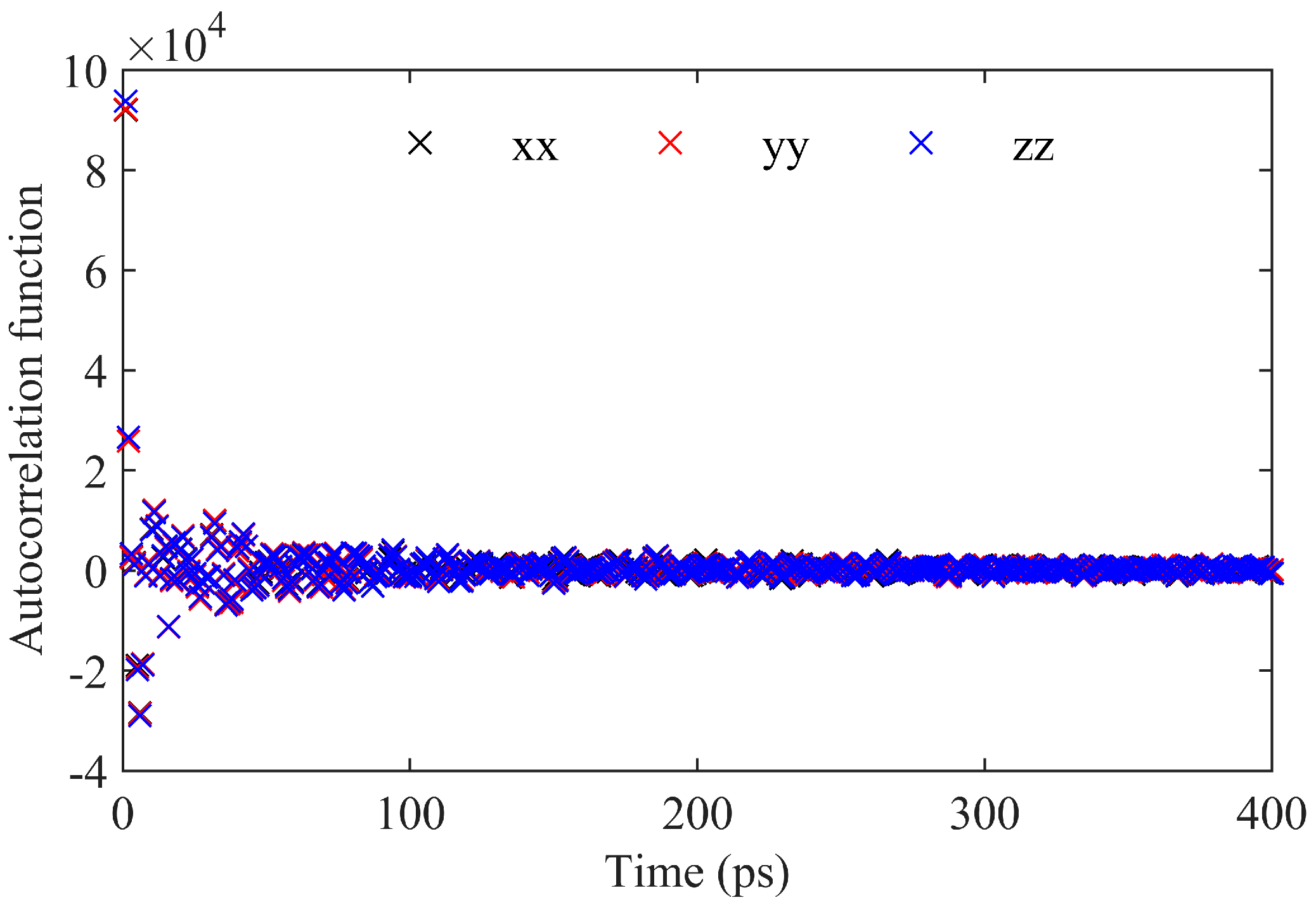
2.1.1. Green–Kubo Integral
2.1.2. Fitting Function
2.1.3. Viscosity Calculation Steps
- (1)
- Under 408.15 K and an NVT ensemble, generating N independent trajectories, which is output using the thermo command in LAMMPS and reflects the changes in atomic positions.
- (2)
- Calculate the asphalt viscosity curves using the GK integration over a total time of 400 ps.
- (3)
- Compute the average and standard deviation of the viscosity integral curves for N trajectories.
- (4)
- Fit the standard deviation to a power-law function, using its reciprocal as the fitting weight.
- (5)
- Utilize Formula (3) to fit the weighted integration and obtain the predicted viscosity value.
- (6)
- Increase the number of trajectories N and repeat steps (1) to (5) until the viscosity calculated in step (5) falls within the error range compared to the previous iteration.
2.2. Reverse Non-Equilibrium Viscosity Calculation
- (1)
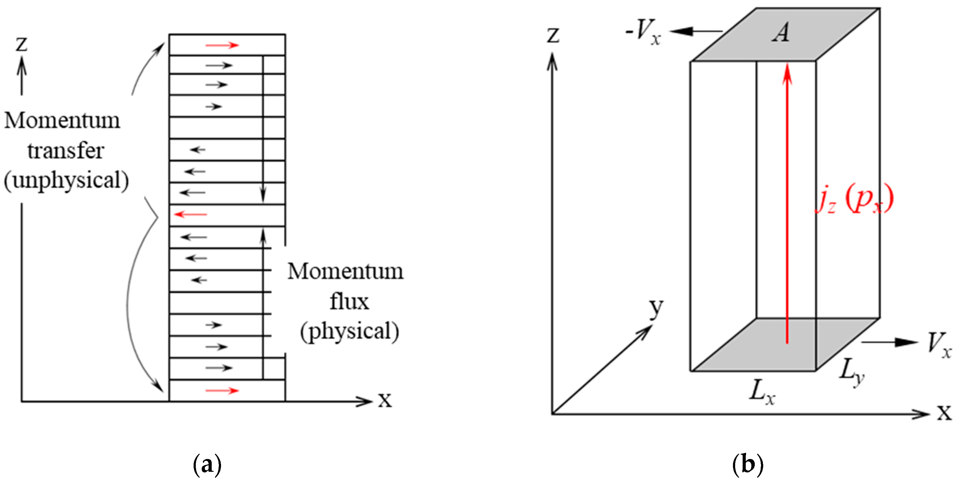
- The periodic box is divided into N (even) regions along the z-direction, as shown in Figure 3a. Atoms in region 1 (the bottommost region) are propelled in the positive x-direction, while atoms in M = N/2 + 1 are propelled in the negative x-direction.
- (2)
- Atoms in region 1 have the maximum x-component momentum in the negative x-direction, and atoms in region M have the maximum x-component momentum in the positive x-direction, with these two atoms having the same mass.
- (3)
- Exchange the x-component of velocities between two corresponding atoms. Since they have the same mass, the exchanged amount is equal to the x-component of momentum.
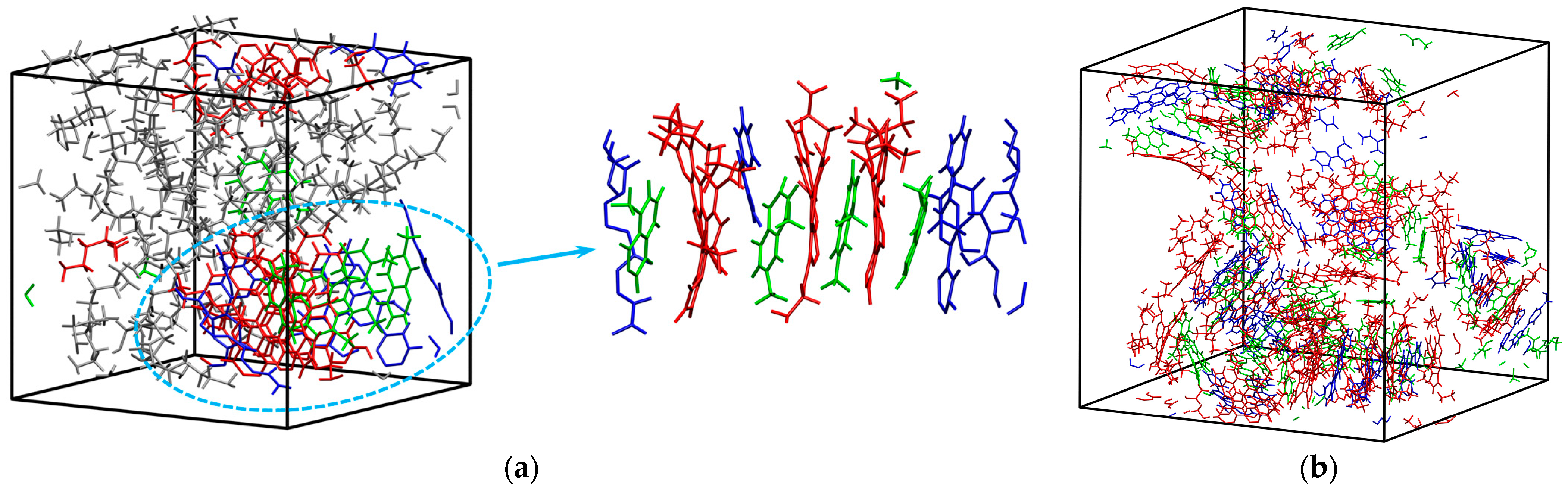
2.3. Modeling and Settings
3. Results and Discussions
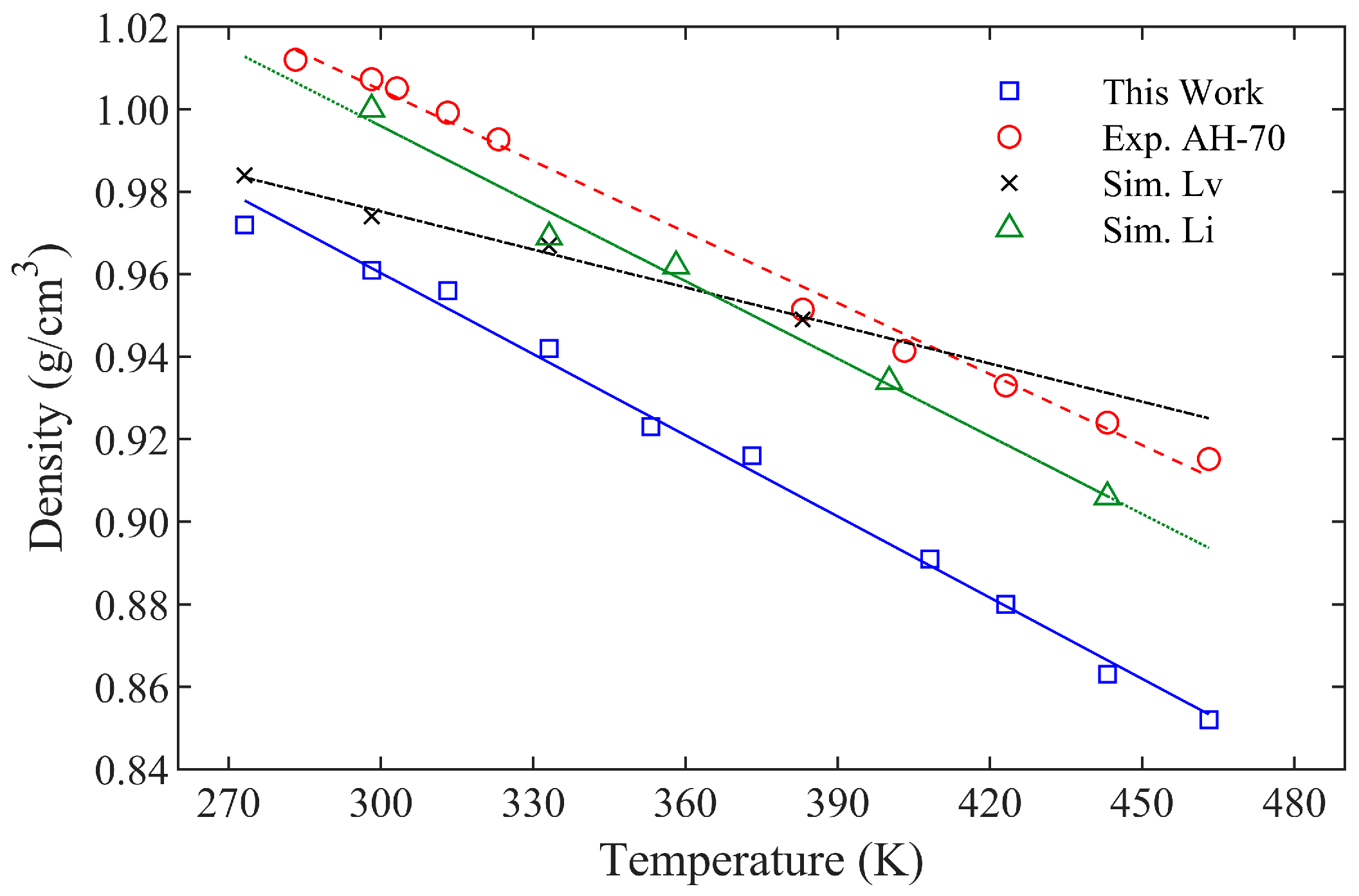
3.1. Density
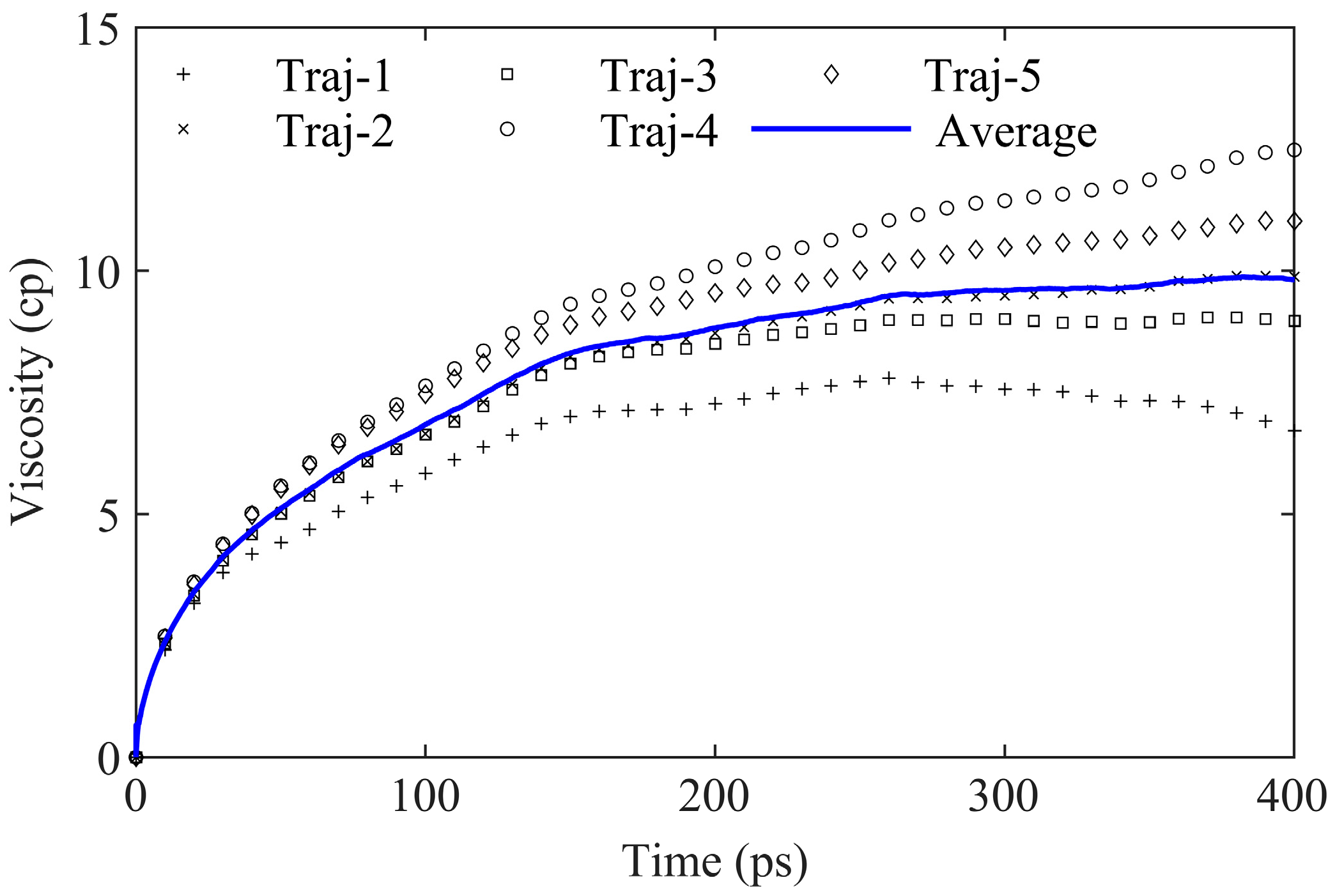
3.2. Equilibrium Viscosity Calculation
3.2.1. Integral Method
3.2.2. Fitting Function
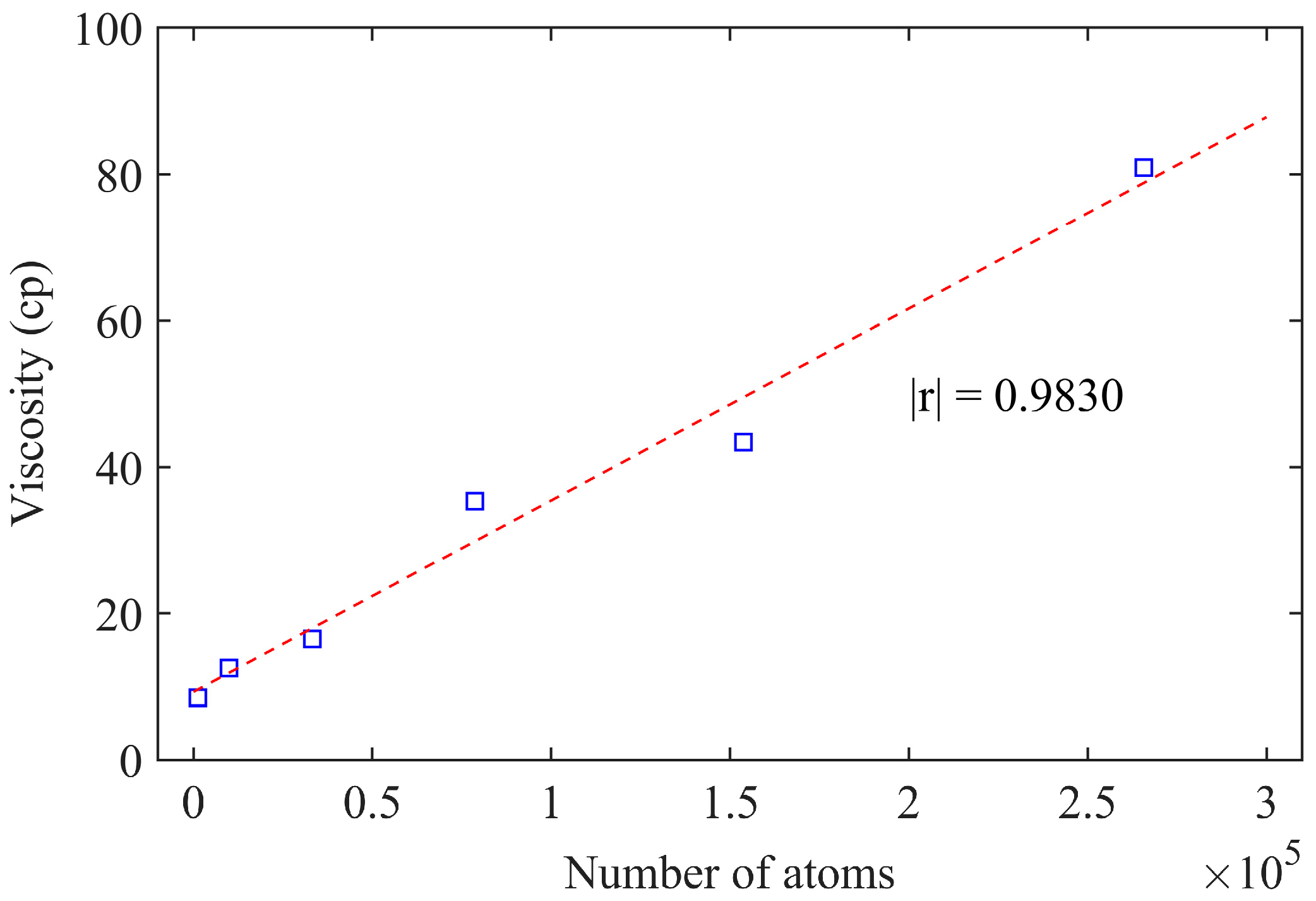
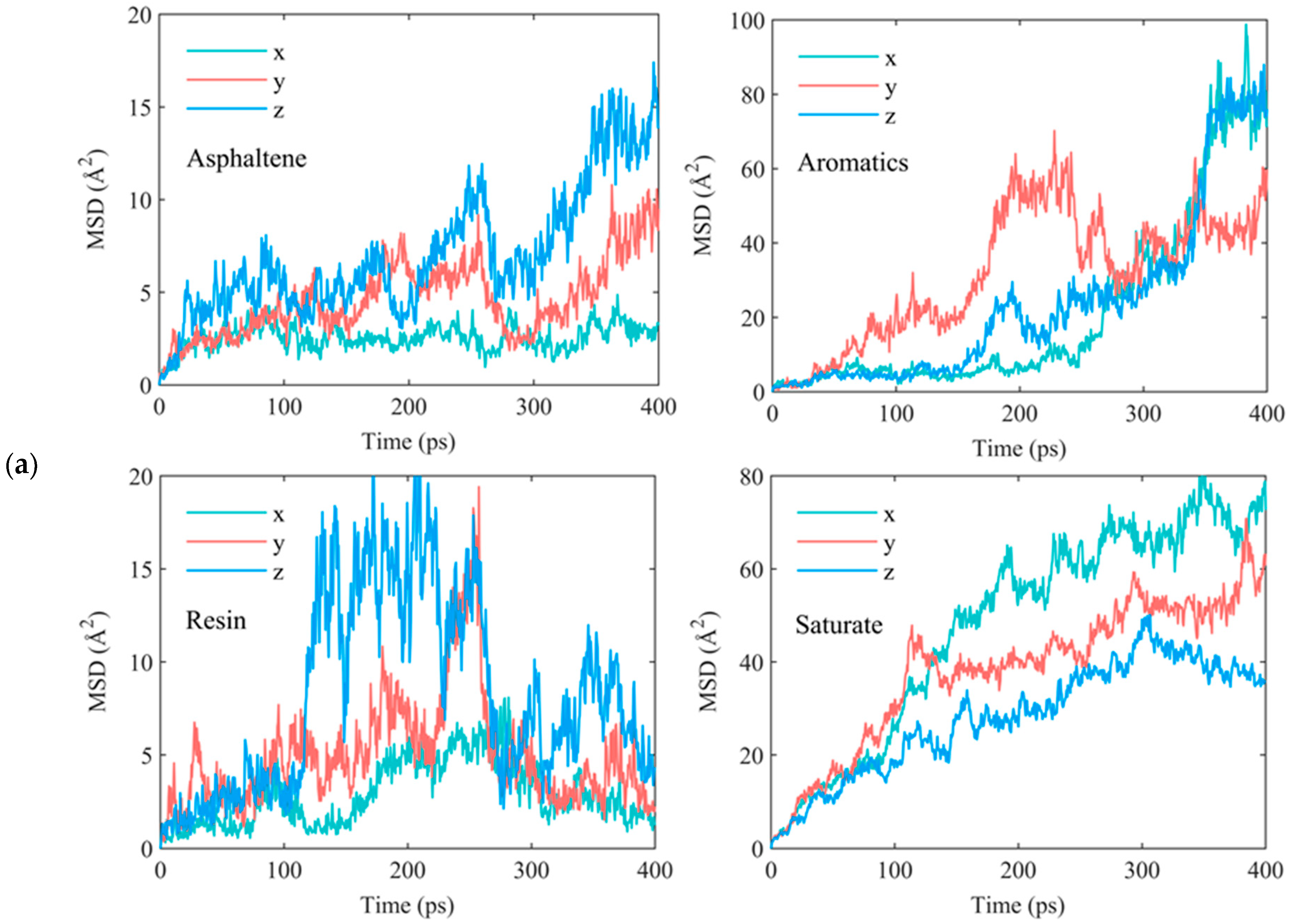
3.2.3. Atomic Number
3.3. Reverse Non-Equilibrium Viscosity Calculation
3.3.1. Number of Regional Divisions
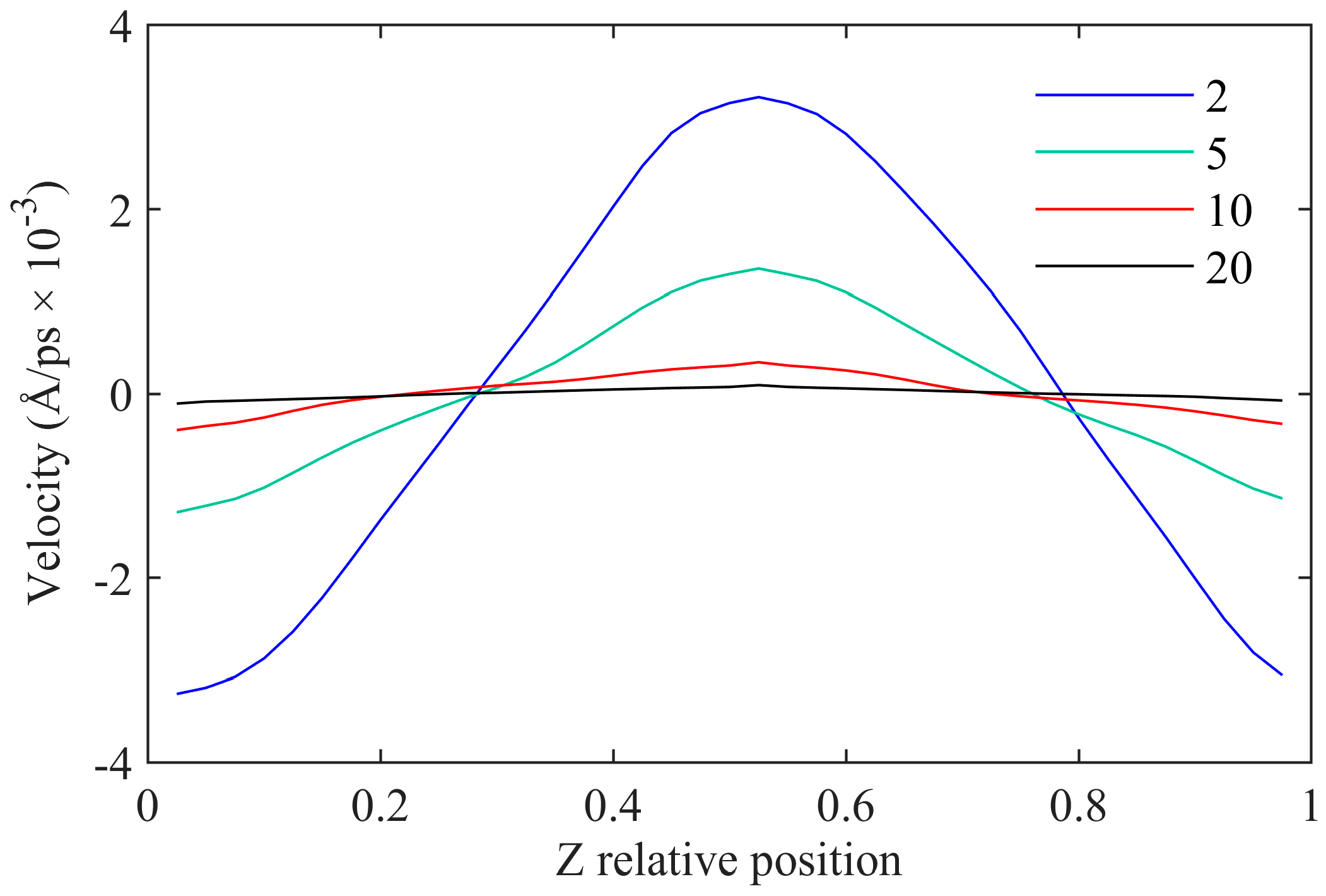
3.3.2. Momentum Exchange Period
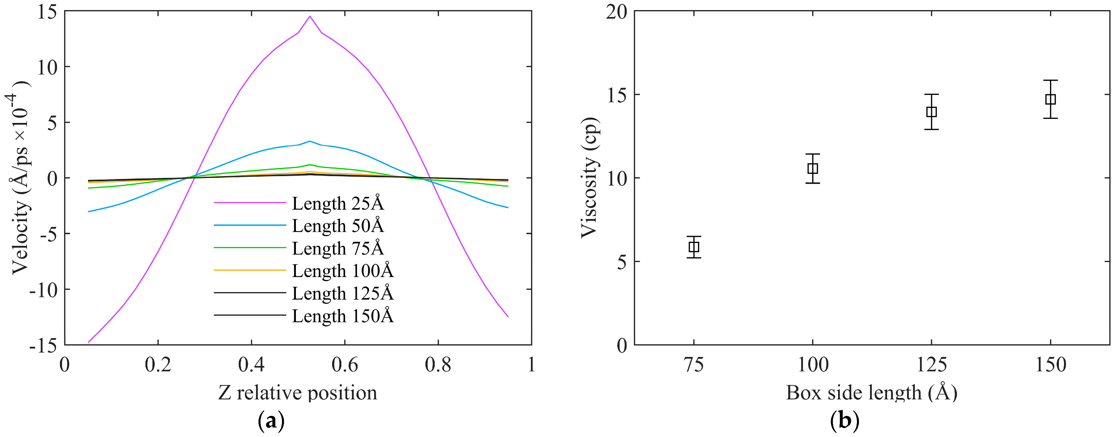
3.3.3. System Size
4. Conclusions
- (1)
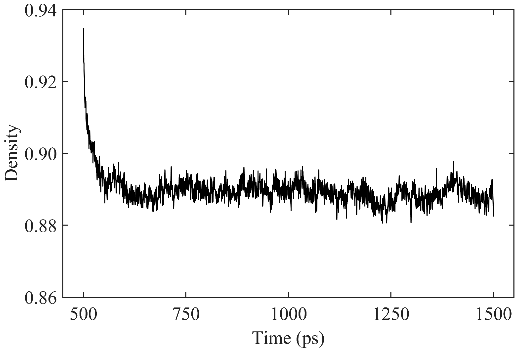
- The Pearson correlation coefficient between asphalt density and temperature exceeds 0.988, indicating a strong linear correlation. At 408.15 K, the asphalt density is 0.891 g/cm3, with an average error of less than 5% compared to experimental values.
- (2)
- In EMD simulations, employing a 1/t weight for viscosity curve calculation results in a well-fitted curve that closely aligns with the original data, demonstrating high precision in the fitting function. The isotropy of the asphalt model improves for atomic counts exceeding 260,000, rendering viscosity calculations more reasonable.
- (3)
- In rNEMD simulations, the number of regions within a certain range has a negligible impact on asphalt viscosity calculation results, with errors being negligible. A momentum exchange period of 20 timesteps exhibits a favorable linear trend in velocity gradients. Using a momentum exchange period within the range of 10 to 20 timesteps is suitable. Larger model sizes demonstrate a more pronounced linear relationship in velocity gradients, and using an orthogonal simulation box with a side length of 75 Å meets the computational requirements effectively.
Author Contributions
Funding
Data Availability Statement
Conflicts of Interest
References
- Luo, Y.; Zhao, X.; Zhang, K.; Shi, X.; Li, G. Research on skid-resistance durability of high viscosity modified asphalt mixture by accelerated abrasion test. Case Stud. Constr. Mater. 2024, 20, e02878. [Google Scholar]
- Hu, Y.; Ryan, J.; Sreeram, A.; Allanson, M.; Pasandín, A.R.; Zhou, L.; Singh, B.; Wang, H.; Airey, G.D. Optimising the dosage of bio-rejuvenators in asphalt recycling: A rejuvenation index based approach. Constr. Build. Mater. 2024, 433, 136761. [Google Scholar] [CrossRef]
- Hu, Y.; Sreeram, A.; Airey, G.D.; Li, B.; Si, W.; Wang, H. Comparative analysis of time sweep testing evaluation methods for the fatigue characterisation of aged bitumen. Constr. Build. Mater. 2024, 432, 136698. [Google Scholar] [CrossRef]
- Yong, F.; Caihua, Y.; Kui, H.; Yujing, C.; Yu, L.; Taoli, Z. A study of the microscopic interaction mechanism of styrene–butadiene-styrene modified asphalt based on density functional theory. Mol. Simul. 2021, 49, 1203–1214. [Google Scholar] [CrossRef]
- Zhang, E.; Shan, L.; Tan, Y. Utilization of Atomic Force Microscopy (AFM) in Characterizing Microscopic Properties of Asphalt Binders: A Review. J. Test. Eval. 2024, 52, JTE20220672. [Google Scholar] [CrossRef]
- Guo, M.; Tan, Y.; Wei, J. Using Molecular Dynamics Simulation to Study Concentration Distribution of Asphalt Binder on Aggregate Surface. J. Mater. Civ. Eng. 2018, 30, 04018075. [Google Scholar] [CrossRef]
- Li, G.; Tan, Y.; Fu, Y.; Liu, P.; Fu, C.; Oeser, M. Density, zero shear viscosity and microstructure analysis of asphalt binder using molecular dynamics simulation. Constr. Build. Mater. 2022, 345, 128332. [Google Scholar] [CrossRef]
- Ding, Y.; Huang, B.; Shu, X. Modeling Shear Viscosity of Asphalt through Nonequilibrium Molecular Dynamics Simulation. Transp. Res. Rec. 2018, 2672, 235–243. [Google Scholar] [CrossRef]
- Yao, H.; Zeng, J.; Liu, J.; Wang, Y.; Li, X.; Dai, Q.; You, Z. Perspectives on the Application of Waste Materials in Asphalt Based on Molecular Dynamics Simulations: A Review. Energy Fuels 2024, 38, 14839–14865. [Google Scholar] [CrossRef]
- Liu, S.; Wang, H.; Yang, J.; Luo, S.; Liu, Y.; Huang, W.; Hu, J.; Xu, G.; Min, Z. Force field benchmark of asphalt materials: Density, viscosity, glass transition temperature, diffusion coefficient, cohesive energy density and molecular structures. J. Mol. Liq. 2024, 398, 124166. [Google Scholar] [CrossRef]
- Wu, M.; Li, M.; You, Z. Asphalt property prediction through high-throughput molecular dynamics simulation. Comput.-Aided Civ. Infrastruct. Eng. 2024. [Google Scholar] [CrossRef]
- Yao, H.; Liu, J.; Xu, M.; Ji, J.; Dai, Q.; You, Z. Discussion on molecular dynamics (MD) simulations of the asphalt materials. Adv. Colloid Interface Sci. 2022, 299, 102565. [Google Scholar] [CrossRef] [PubMed]
- Plimpton, S. Fast Parallel Algorithms for Short-Range Molecular Dynamics. J. Comput. Phys. 1995, 117, 1–19. [Google Scholar] [CrossRef]
- Tenney, C.M.; Maginn, E.J. Limitations and recommendations for the calculation of shear viscosity using reverse nonequilibrium molecular dynamics. J. Chem. Phys. 2010, 132, 014103. [Google Scholar] [CrossRef]
- Zhang, L.; Greenfield, M.L. Relaxation time, diffusion, viscosity analysis of model asphalt systems using molecular simulation. J. Chem. Phys. 2007, 127, 194502. [Google Scholar] [CrossRef] [PubMed]
- Mercier Franco, L.F.; Firoozabadi, A. Computation of Shear Viscosity by a Consistent Method in Equilibrium Molecular Dynamics Simulations: Applications to 1-Decene Oligomers. J. Phys. Chem. B 2023, 127, 10043–10051. [Google Scholar] [CrossRef]
- Toraman, G.; Verstraelen, T.; Fauconnier, D. Impact of Ad Hoc Post-Processing Parameters on the Lubricant Viscosity Calculated with Equilibrium Molecular Dynamics Simulations. Lubricants 2023, 11, 183. [Google Scholar] [CrossRef]
- Evans, D.J.; Morriss, G.P. Nonlinear-response theory for steady planar Couette flow. Phys. Rev. A 1984, 30, 1528–1530. [Google Scholar] [CrossRef]
- Gao, Y.; Wu, J.; Feng, Y.; Han, J.; Fang, H. Structural effects of water clusters on viscosity at high shear rates. J. Chem. Phys. 2024, 160, 104502. [Google Scholar] [CrossRef]
- Shen, M.; Zhang, F.; Liu, Y.; Zhou, X. Molecular dynamics study on the viscosity of hydraulic oil in the deep-sea environment. J. Mol. Liq. 2024, 411, 125716. [Google Scholar] [CrossRef]
- Bordat, P.; Müller-Plathe, F. The shear viscosity of molecular fluids: A calculation by reverse nonequilibrium molecular dynamics. J. Chem. Phys. 2002, 116, 3362–3369. [Google Scholar] [CrossRef]
- Müller-Plathe, F. Reversing the perturbation in nonequilibrium molecular dynamics: An easy way to calculate the shear viscosity of fluids. Phys. Rev. E—Stat. Phys. Plasmas Fluids Relat. Interdiscip. Top. 1999, 59, 4894–4898. [Google Scholar] [CrossRef]
- You, L.; Spyriouni, T.; Dai, Q.; You, Z.; Khanal, A. Experimental and molecular dynamics simulation study on thermal, transport, and rheological properties of asphalt. Constr. Build. Mater. 2020, 265, 120358. [Google Scholar] [CrossRef]
- Jagannathan, A.; Oono, Y.; Schaub, B. Intrinsic viscosity from the Green–Kubo formula. J. Chem. Phys. 1987, 86, 2276–2285. [Google Scholar] [CrossRef]
- Rey-Castro, C.; Vega, L.F. Transport properties of the ionic liquid 1-ethyl-3-methylimidazolium chloride from equilibrium molecular dynamics simulation. The effect of temperature. J. Phys. Chem. B 2006, 110, 14426–14435. [Google Scholar] [CrossRef]
- Cheng, Y.; Wang, H.; Wang, S.; Gao, X.; Li, Q.; Fang, J.; Song, H.; Chu, W.; Zhang, G.; Song, H. Deep-learning potential method to simulate shear viscosity of liquid aluminum at high temperature and high pressure by molecular dynamics. AIP Adv. 2021, 11, 015043. [Google Scholar] [CrossRef]
- Zhang, Y.; Otani, A.; Maginn, E.J. Reliable viscosity calculation from equilibrium molecular dynamics simulations: A time decomposition method. J. Chem. Theory Comput. 2015, 11, 3537–3546. [Google Scholar] [CrossRef] [PubMed]
- Hess, B. Determining the shear viscosity of model liquids from molecular dynamics simulations. J. Chem. Phys. 2002, 116, 209–217. [Google Scholar] [CrossRef]
- Nie, Y.; Zhan, H.; Kou, L.; Gu, Y. Atomistic Insights on the Rheological Property of Polycaprolactone Composites with the Addition of Graphene. Adv. Mater. Technol. 2022, 7, 2100507. [Google Scholar] [CrossRef]
- Krieger, J.B.; Iafrate, G.J. Time evolution of Bloch electrons in a homogeneous electric field. Phys. Rev. B 1986, 33, 5494–5500. [Google Scholar] [CrossRef]
- Yao, H.; Dai, Q.; You, Z. Molecular dynamics simulation of physicochemical properties of the asphalt model. Fuel 2016, 164, 83–93. [Google Scholar] [CrossRef]
- Nie, F.; Jian, W.; Lau, D. An atomistic study on the thermomechanical properties of graphene and functionalized graphene sheets modified asphalt. Carbon 2021, 182, 615–627. [Google Scholar] [CrossRef]
- Tarefder, H.R.A. Temperature and Moisture Impacts on Asphalt before and after Oxidative Aging Using Molecular Dynamics Simulations. J. Nanomech. Micromech. 2017, 7, 04017018. [Google Scholar]
- Hockney, R.W.; Eastwood, J.W. Computer Simulation Using Particles; CRC Press: Boca Raton, FL, USA, 2021. [Google Scholar]
- Bussi, G.; Donadio, D.; Parrinello, M. Canonical sampling through velocity rescaling. J. Chem. Phys. 2007, 126, 014101. [Google Scholar] [CrossRef]
- Williams, M.L.; Landel, R.F.; Ferry, J.D. The Temperature Dependence of Relaxation Mechanisms in Amorphous Polymers and Other Glass-Forming Liquids. J. Am. Chem. Soc. 1955, 77, 3701–3707. [Google Scholar] [CrossRef]
- Zhao, L.; Choi, P. Study of the correctness of the solubility parameters obtained from indirect methods by molecular dynamics simulation. Polymer 2004, 45, 1349–1356. [Google Scholar] [CrossRef]
- Hu, Y.; Sreeram, A.; Xia, W.; Wang, H.; Zhou, L.; Si, W.; Airey, G.D. Use of Hansen Solubility Parameters (HSP) in the selection of highly effective rejuvenators for aged bitumen. Road Mater. Pavement Des. 2024, 1–19. [Google Scholar] [CrossRef]
- Lesueur, D. The colloidal structure of bitumen: Consequences on the rheology and on the mechanisms of bitumen modification. Adv. Colloid Interface Sci. 2009, 145, 42–82. [Google Scholar] [CrossRef] [PubMed]
- Qu, X.; Liu, Q.; Guo, M.; Wang, D.; Oeser, M. Study on the effect of aging on physical properties of asphalt binder from a microscale perspective. Constr. Build. Mater. 2018, 187, 718–729. [Google Scholar] [CrossRef]
- Zhang, L.; Greenfield, M.L. Rotational relaxation times of individual compounds within simulations of molecular asphalt models. J. Chem. Phys. 2010, 132, 184502. [Google Scholar] [CrossRef]
- Kelkar, M.S.; Rafferty, J.L.; Maginn, E.J.; Siepmann, J.I. Prediction of viscosities and vapor–liquid equilibria for five polyhydric alcohols by molecular simulation. Fluid Phase Equilibria 2007, 260, 218–231. [Google Scholar] [CrossRef]
- Zhang, X.; Qian, C.; Zhou, L.; Zhang, Y. Predict low-temperature properties of asphalt from the relationsip between density and temperature. Pet. Asph. 2009, 23, 67–71. [Google Scholar]
- Lv, Z.; Pan, L.; Zhang, J.; Lin, X. Molecular Dynamics Simulation of Adhension Mechanism of Asphalt-aggregate Interface. J. Mater. Sci. Eng. 2022, 40, 809–815+834. [Google Scholar]
- Li, D.D.; Greenfield, M.L. Chemical compositions of improved model asphalt systems for molecular simulations. Fuel 2014, 115, 347–356. [Google Scholar] [CrossRef]
- Li, D.D.; Greenfield, M.L. Viscosity, relaxation time, and dynamics within a model asphalt of larger molecules. J. Chem. Phys. 2014, 140, 034507. [Google Scholar] [CrossRef] [PubMed]
- Van-Oanh, N.-T.; Houriez, C.; Rousseau, B. Viscosity of the 1-ethyl-3-methylimidazolium bis (trifluoromethylsulfonyl) imide ionic liquid from equilibrium and nonequilibrium molecular dynamics. Phys. Chem. Chem. Phys. 2010, 12, 930–936. [Google Scholar] [CrossRef] [PubMed]
- He, L.; Li, G.; Zheng, Y.; Alexiadis, A.; Valentin, J.; JKowalski, K. Research Progress and Prospect of Molecular Dynamics of Asphalt Systems. Mater. Rep. 2020, 34, 19083–19093. [Google Scholar]
- Tan, Y.; LI, G.; Shan, L.; Lyu, H.; Meng, A. Research Progress of Bitumen Microstructure and components. J. Traffic Transpotation Eng. 2020, 20, 1–17. [Google Scholar]


| Asphalt Molecule | Chemical Formula | Mass (g/mol) | Mass Ratio (%) |
|---|---|---|---|
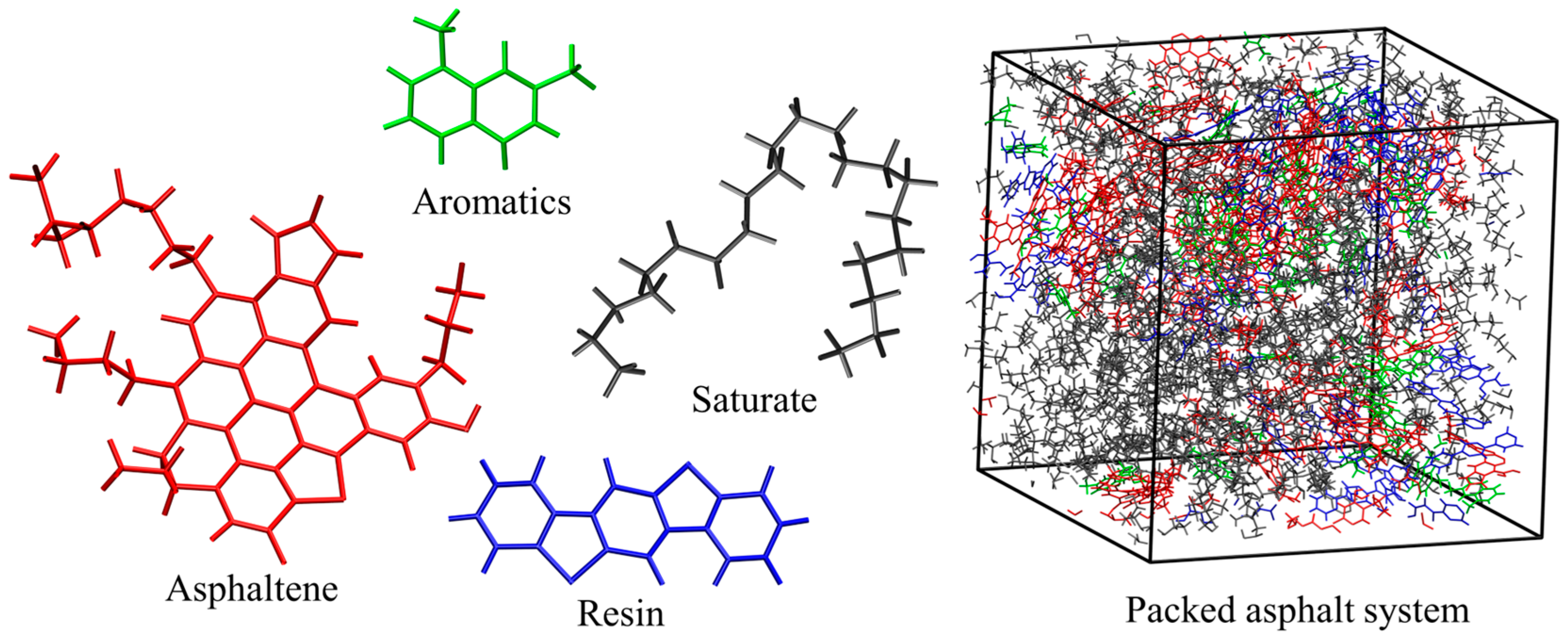
| Asphaltene | C53H55NOS | 754.04 | 26 |
| Aromatics | C12H12 | 156.22 | 8 |
| Resin | C18H10S2 | 290.38 | 17 |
| Saturate | C22H46 | 310.59 | 49 |
| Asphalt System | Regression Equation between Density and Temperature | Correlation Coefficient |
|---|---|---|
| This Work | ρ = −0.0007 T + 1.157 | 0.9938 |
| Exp. AH-70 [43] | ρ = −0.0006 T + 1.022 | 0.9968 |
| Sim. Lv [44] | ρ = −0.0003 T + 1.068 | 0.9881 |
| Sim. Li [45] | ρ = −0.0006 T + 1.084 | 0.9895 |
| Model | Side Length (Å) | Density (g/cm3) | Number of Molecules | Number of Atoms | Viscosity (cp) | |||
|---|---|---|---|---|---|---|---|---|
| Asphaltene | Resin | Aromatic | Saturate | |||||
| M-1 | 25 | 0.858 | 3 | 5 | 5 | 15 | 1183 | 8.52 |
| M-2 | 50 | 0.895 | 26 | 38 | 44 | 120 | 9898 | 12.52 |
| M-3 | 75 | 0.891 | 86 | 129 | 148 | 406 | 33,224 | 16.52 |
| M-4 | 100 | 0.893 | 204 | 306 | 350 | 962 | 78,712 | 35.36 |
| M-5 | 125 | 0.893 | 399 | 598 | 683 | 1879 | 153,769 | 43.43 |
| M-6 | 150 | 0.893 | 689 | 1033 | 1181 | 3247 | 265,705 | 80.94 |
Disclaimer/Publisher’s Note: The statements, opinions and data contained in all publications are solely those of the individual author(s) and contributor(s) and not of MDPI and/or the editor(s). MDPI and/or the editor(s) disclaim responsibility for any injury to people or property resulting from any ideas, methods, instructions or products referred to in the content. |
© 2024 by the authors. Licensee MDPI, Basel, Switzerland. This article is an open access article distributed under the terms and conditions of the Creative Commons Attribution (CC BY) license (https://creativecommons.org/licenses/by/4.0/).
Share and Cite
Hu, X.; Huang, X.; Zhou, Y.; Zhang, J.; Lu, H. Viscosity of Asphalt Binder through Equilibrium and Non-Equilibrium Molecular Dynamics Simulations. Buildings 2024, 14, 2827. https://doi.org/10.3390/buildings14092827
Hu X, Huang X, Zhou Y, Zhang J, Lu H. Viscosity of Asphalt Binder through Equilibrium and Non-Equilibrium Molecular Dynamics Simulations. Buildings. 2024; 14(9):2827. https://doi.org/10.3390/buildings14092827
Chicago/Turabian StyleHu, Xiancheng, Xiaohan Huang, Yuanbin Zhou, Jiandong Zhang, and Hongquan Lu. 2024. "Viscosity of Asphalt Binder through Equilibrium and Non-Equilibrium Molecular Dynamics Simulations" Buildings 14, no. 9: 2827. https://doi.org/10.3390/buildings14092827
APA StyleHu, X., Huang, X., Zhou, Y., Zhang, J., & Lu, H. (2024). Viscosity of Asphalt Binder through Equilibrium and Non-Equilibrium Molecular Dynamics Simulations. Buildings, 14(9), 2827. https://doi.org/10.3390/buildings14092827