Article

An Explainable Machine Learning-Based Prediction of Backbone Curves for Reduced Beam Section Connections Under Cyclic Loading

1
College of Engineering and Technology, American University of the Middle East, Egaila 54200, Kuwait
2
Civil & Environmental Engineering Department, University of California, Los Angeles, CA 90095, USA
*
Author to whom correspondence should be addressed.
Buildings 2025, 15(13), 2307; https://doi.org/10.3390/buildings15132307
Submission received: 3 June 2025 / Revised: 25 June 2025 / Accepted: 26 June 2025 / Published: 30 June 2025

Abstract

Reduced Beam Sections (RBS) are used in steel design to promote ductile behavior by shifting inelastic deformation away from critical joints, enhancing seismic performance through controlled energy dissipation. While current design guidelines assist in detailing RBS connections, moment–rotation curves—essential for understanding energy dissipation—require extensive testing and/or modeling. Machine learning (ML) offers a promising alternative for predicting these curves, yet few studies have explored ML-based approaches, and none, to the best of the authors’ knowledge, have applied Explainable Artificial Intelligence (XAI) to interpret model predictions. This study presents an ML framework using Artificial Neural Networks (ANN), Random Forest (RF), Support Vector Machines (SVM), Gradient Boosting (GB), and Ridge Regression (RR) trained on 500 numerical models to predict the moment–rotation backbone curve of RBS connections under cyclic loading. Among all the models applied, the ANN obtained the highest R2 value of 99.964%, resulting in superior accuracy. Additionally, Shapley values from XAI are employed to evaluate the influence of input parameters on model predictions. The average SHAP values provide important insights into the performance of RBS connections, revealing that cross-sectional characteristics significantly influence moment capacity. In particular, flange thickness (tf), flange width (bf), and the parameter “c” are critical factors, as the flanges contribute the most substantially to resisting bending moments.

1. Introduction

Beam-to-column connections are critical components of buildings as connections transfer loads between beams and columns, making it essential to design them to withstand severe loads without failure. In moment-resisting building frames, beam-to-column connections are typically constructed by welding beam flanges to the column face. Since the energy input during earthquakes is expected to be dissipated through plastic hinge formation in beams near the column flange surface, the welds must be strong enough to endure severe stress–strain cycles. Many welded steel moment-resisting frames suffered damage during the 1994 Northridge earthquake [1,2]. Even though the total collapse of buildings was not observed due to connection failures, the sudden (brittle) failure of welds in the steel–beam connection resulted in significant repair costs [3]. Due to this unexpected failure mode, the SAC joint venture, supported by FEMA, investigated the development of state-of-the-art solutions for buildings constructed before the Northridge earthquake and recommended a set of seismic design criteria for new buildings [1]. Various connection types were developed and implemented after the Northridge earthquake [3]. These connections can be categorized into connections with reinforcements, such as top cover plates and haunches, and connections with Reduced Beam Sections (RBS). The latter involved the intentional weakening of the beam flanges by trimming a portion of the flange near the column face, thus shifting plastic deformation away from the weld region to prevent brittle failure.

1.1. RBS Connections in the Literature

Several research studies have been conducted, both experimentally and numerically, to enhance the understanding of the seismic performance of RBS connections in moment-resisting frames. A comprehensive summary of these studies is given in Table 1. Uang et al. [4] experimentally investigated the impact of RBS and welded haunches on the cyclic behavior of steel moment connections, both with and without concrete slabs. The results showed that while RBS improved connection performance when low-toughness welds were replaced, the welded haunches significantly enhanced cyclic performance, achieving a plastic rotation of 0.027 rad when a concrete slab was included. Chen and Chao [5] experimentally demonstrated that a beam-to-column connection with RBS could achieve an average plastic rotation of 0.045 rad, exceeding the performance of typical steel beam-to-column connections when floor slabs were included. However, unsymmetrical stress, induced by floor slabs, caused weld fractures in the bottom flange, highlighting the critical importance of weld quality. Gilton and Uang [6] conducted experimental and numerical studies to investigate the cyclic behavior of weak-axis RBS moment connections. The experimental results demonstrated that the connections could achieve the required plastic rotation of 0.03 rad without exhibiting brittle weld failures. Furthermore, finite element (FE) models revealed that strain concentrations could be reduced by a factor of three compared to connections without RBS. Lee et al. [7] investigated the seismic behavior of RBS steel moment connections through the experimental testing of eight beam-to-column specimens with varying parameters, including panel zone strength and the method (weld or bolt) used to connect the beam web to the column face. The specimen with a welded web connection and a medium panel zone strength ratio achieved acceptable rotation capacity, whereas bolted web specimens experienced premature fracture at the welded access hole of the beam flange. In another study, Lee and Kim [8] investigated RBS moment connections with bolted webs, highlighting that these connections failed due to premature fractures at the weld access holes triggered by bolt slippage and having a load transfer mechanism different than that of the assumed connection design. An improved design procedure demonstrated that the specimen could achieve a 5% story drift without any observed damage. Pachoumis et al. [9] investigated the application of RBS connections to European steel beam profiles commonly used in practice through experimental and numerical methods. Both experimental tests and numerical models showed that RBS connections can exhibit significant cyclic performance by reaching a plastic rotation of 0.03 rad. In their research study, Ohsaki et al. [10] developed a simulated annealing optimization approach using finite element models calibrated with experimental tests, intending to maximize energy dissipation at the Reduced Beam Section (RBS) while constraining the maximum equivalent plastic strain at the critical weld region. The results demonstrated that the optimal design effectively shifts plastic deformation away from the critical weld region. Pachoumis et al. [11] conducted an experimental and numerical study using RBS details that did not conform to EC8 and FEMA geometrical recommendations, demonstrating plastic rotations exceeding 0.03 rad without damage to the critical weld region. Han et al. [12] conducted a study on the rotation capacity of RBS with bolted webs as the connections designed according to AISC 358-16 [13] suffered damage at rotations below 0.02 rad in previous research studies. An empirical design equation, considering parameters such as beam depth, moment strength ratio, and yield strength normalized by Young’s modulus, was developed to ensure a rotation capacity exceeding 0.02 rad. Sofias et al. [14] examined the behavior of Reduced Beam Section (RBS) moment connections with extended bolted end plates through experimental testing and numerical modeling, using beams of different steel grades but identical radius cut RBS geometries. The experimental results demonstrated that both beams exceeded the expected rotation capacity of 0.03 rad without causing damage to connection elements such as bolts, the end plate, weld, and column flange. Oh et al. [15] experimentally investigated weak-axis column-tree moment connections featuring RBS and tapered beams to evaluate their rotation capacity, energy dissipation capacity, and ductility. Although both beam configurations met the expected performance criteria outlined in the design code by achieving a 5% drift capacity without brittle fracture, the RBS specimen demonstrated superior energy dissipation and more stable ductile behavior. Li et al. [16] experimentally examined the cyclic performance of composite joints with RBS connected to concrete-filled tubular (CFT) columns including slabs. Six specimens were tested to analyze the effects of RBS and slabs on joints by analyzing strength, stiffness degradation, ductility, and strain development. A numerical investigation of an innovative steel moment connection, named the Double Reduced Beam Section (DRBS) connection, was conducted by Morshedi et al. [17]. This concept incorporates double dog-bone sections to expand the plastic hinge region, thus reducing the equivalent plastic strain. Their research exhibited that the DRBS outperformed conventional RBS connections, increasing deformation capacity by up to 40% and reducing equivalent plastic strain by 35–60%. Sophianopoulos and Deri [18] developed an optimization methodology for RBS connections using European steel profiles, focusing on static loading to ensure ductility and plastic hinge formation. The focus was on preventing premature failure through regression analysis and numerical optimization to derive optimal designs. Eight optimal designs were generated, meeting both static and seismic design requirements. In their study, Liu et al. [19] proposed a buckling-restrained RBS connection to prevent the local buckling of the flanges and web under compression. Experimental and numerical analyses demonstrated that the stability and stiffness of the beam–column assembly could be maintained up to a 5.5% story drift. Horton et al. [20] conducted a comprehensive study to identify the key parameters influencing the seismic performance of RBS connections. Using 90 finite element (FE) models that accounted for geometrical parameters, their study revealed that the depth “c” of the RBS cut had a significant impact on seismic design parameters, including yield moment, peak moment, ductility, and energy dissipation. Empirical design equations were subsequently developed to predict these seismic design parameters. In a subsequent study, Horton et al. [21] developed a comprehensive and accurate database of modified Ibarra–Krawinkler (mIK) models for American wide-flange beams with RBS connections, addressing the challenges of accurately modeling the hysteretic behavior of RBS connections under seismic loading. A total of 1480 finite element (FE) models were created to determine mIK parameters and capture the cyclic response of beams in OpenSees. This study revealed that the depth “c” of the RBS cut has a substantial impact on buckling in beam sections with slender webs, as well as on the yield moment and initial stiffness. Ozkilic and Bozkurt [22] proposed a replaceable RBS connection for moment-resisting frames to simplify repairs after severe seismic events. The RBS connection was designed to be bolted to the column face using end plates and to the main beam using side plates through the channel section connected to the RBS. Numerical investigations using finite element (FE) models demonstrated that the proposed connection met all the requirements of AISC 341-16 [13]. Yao et al. [23] developed a novel Reduced Beam Section (RBS) steel composite frame beam aimed at improving seismic resilience and facilitating post-earthquake damage control. Experimental and FE analyses revealed that the innovative connections enhance the energy dissipation and stiffness of the frame compared to conventional steel frame designs while reducing steel usage by up to 12.3%. Based on the findings from the experiments and FE models, seismic design requirements were proposed.

1.2. Use of Machine Learning in Structural Engineering

Machine learning (ML) techniques offer a promising alternative for complex structural systems under extreme conditions with extremely nonlinear behavior, as traditional structural analysis and design methods are often overly complex and laborious for practical implementation [24]. Numerous studies have been conducted using state-of-the-art ML techniques including Random Forest (RF), Decision Trees (DTs), XGBoost (XB), CatBoost (CB), AdaBoost (AB), k-Nearest Neighbors (KNNs), Support Vector Machines (SVM), Artificial Neural Networks (ANN), Ridge Regression (RR), Lasso Regression (LR2), and Regression Analysis (RA) [25,26,27,28,29,30,31,32]. Rahman et al. [32] used ML to predict the shear strength of steel fiber-reinforced concrete (SFRC) beams using machine learning models on a dataset of 507 experimentally tested beams. Eleven ML models were evaluated, with XB ultimately demonstrating the highest prediction performance. Their study identified key factors affecting shear capacity, such as the reinforcement ratio, fiber volume, and span-to-depth ratio, emphasizing the potential of ML to improve structural design methodologies for SFRC. De Oliveira et al. [28] investigated the prediction of lateral–torsional buckling in steel–concrete composite cellular beams using ML, including the use of ANN, RF, XB, and SVM. Their study used a dataset of 458 beam results derived from experimentally calibrated finite element (FE) models. Though all ML models achieved R2 values above 0.90, XB was identified as the best-performing model based on its correlation coefficient and mean squared error. Liu et al. [30] presented research on predicting the bending moment resistance of high-strength steel welded I-section beams using ML models. Five machine learning models, including random forest regressor (RFR), SVM, ANN, Linear Regression, and XB, were utilized in this research, with XB demonstrating superior performance in the prediction of the bending moment. The findings of this study revealed that the ML models provided more accurate predictions compared to code-suggested design methods, highlighting the potential of ML to improve the structural design of high-strength steel welded I-section beams. Marie et al. [31] employed six ML models, including Ordinary Least Squares (OLS), Multivariate Adaptive Regression Splines (MARS), SVM, KNNs, ANN, and Kernel Regression, to predict the shear strength of beam–column joints using a dataset comprising 98 experimentally tested joint specimens. The results of the ML prediction framework revealed that Kernel Regression achieved the highest prediction accuracy, with an R2 value of 0.97. This research emphasized the potential of ML models to facilitate the structural design of such joints without the need for labor-intensive experimental methods. Dabiri et al. [27] predicted the displacement ductility ratio of RC beam–column joints using both regression-based and ML-based models, utilizing a database of over 170 experimental test results from peer-reviewed studies. While all models achieved an R2 value greater than 0.76, the nonlinear regression method demonstrated the highest accuracy with an R2 value of 0.90. The findings suggested that regression-based and ML-based models can serve as efficient alternatives to time-intensive experimental and numerical methods for predicting displacement ductility ratios. The shear strength of short links in steel structures was investigated by Almasabha et al. [25] using ML, including the Light Gradient Boosting Machine (LightGBM), XB, and ANN. All the ML models achieved an R2 value of 0.90 or higher, demonstrating significantly more accurate predictions than those of the traditional design codes used for short links. Among all models considered in this study, LightGBM achieved the most accurate predictions. SVM, multilayer perceptron (MLP), Gradient Boosting Regressor (GBR), and XB were successfully utilized by Dissanayake et al. [29] to predict the shear capacity of both stainless-steel lipped channel sections and carbon steel LiteSteel sections. SVR was the most accurate model with an R2 value of 0.999 and a Mean Absolute Error (MAE) value of %2.32. This study also showed that ML models can have more accurate predictions than the codified design calculation. Avci-Karatas [26] conducted a research study on the shear capacity prediction of headed shear steel studs in steel–concrete composite structures using ML models with Minimax Probability Machine Regression (MPMR) and Extreme Machine Learning (EML). The MPMR model reached an R2 value of 0.9913, and the EML model achieved an R2 value of 0.9479, indicating high prediction accuracy when compared to experimental data.
Although ML has been extensively used in previous studies as a prediction method, a limited number of studies are focusing on RBS connections. Horton et al. [33] developed a novel deep learning neural network to determine the parameters required for the modified Ibarra–Krawinkler (mIK) hysteretic model for RBS connections based on their previous studies [21]. The proposed approach utilized the geometrical dimensions of RBS connections to make precise predictions, with the networks trained on a robust database of 1480 FE models developed on American wide-flange sections. The developed ML framework achieved a classification accuracy of 96% for distinguishing between buckle and non-buckle characteristics, and the mIK parameters were predicted with an accuracy of 98%. A comprehensive literature summary of ML and XAI integrated studies can be found in Table 2.
As the field of structural engineering continues to evolve, the reliance on computational models such as ML has become increasingly prevalent. These models, often powered by advanced algorithms and datasets, are instrumental in predicting the behavior and performance of structures under various loading conditions. However, the growing complexity of these models has raised concerns about their interpretability and explainability, which are crucial for ensuring the reliability of structural engineering decision-making. In the absence of explanations, models are “black boxes,” and diagnosing errors and detecting biases become challenging. In structural engineering, explainable AI (XAI) is essential for ensuring the use of these models while designing and analyzing infrastructures. Unlike traditional physics-based methods, AI models rely on data-driven models that may not always be interpretable. Explainability helps engineers understand why a model predicts certain outcomes, allowing them to validate results, detect potential biases, and refine models to align with real-world engineering principles. Moreover, engineers must adhere to strict regulatory codes, and XAI ensures that AI-driven insights can be justified and aligned with these standards. It also aids in debugging models, optimizing designs, and quantifying uncertainties in construction materials, environmental conditions, and load variations. By leveraging techniques such as feature importance analysis, rule-based AI models, and physics-informed AI, structural engineers can integrate AI more effectively into their workflows [34,35,36,37]. However, explainability and XAI methods have limited applications in structural engineering, and to the best of the authors’ knowledge, they have not been used in RBS and moment–rotation curve predictions. Mangalathu et al. [38] developed XAI models using a Random Forest algorithm to predict the failure modes of reinforced concrete (RC) columns and shear walls, aiming to enhance the interpretability of complex machine learning models to facilitate their adoption. They adopted the Shapley Additive Explanations (SHAP) approach to identify the most influential parameters and explain how the ML models predict a specific failure mode for a given dataset. Their study revealed that geometric parameters are the most critical factors influencing failure modes in RC columns and shear walls. The Random Forest ML models yielded 84% accuracy for columns, whereas 86% accuracy was achieved for shear walls. Wakjira et al. [39] also utilized the SHAP approach to explain ML models and determine the most significant parameters affecting the Plastic Hinge Length (PHL) of rectangular RC columns. Five machine learning models, including XGBoost, were adopted for prediction. The results demonstrated that these machine learning models outperformed existing empirical models, providing superior accuracy in PHL estimation. Among all the machine learning models used, XGBoost demonstrated the highest performance, achieving an R2 of 98% in prediction accuracy. In their research work, Angelucci et al. [40] predicted displacement demand in RC buildings under pulse-like earthquakes using an interpretable ML framework. Gaussian Process Regression (GPR) was used to identify key aspects, such as building attributes and intensity measures, while Genetic Programming (GP) was employed to develop a reduced-scale ML model using a reduced set of intensity measures selected via the SHAP approach, which enhances interpretability and aids in the rational selection of intensity measures. Zhu et al. [41] developed an XAI model to predict the shear bearing capacity of a fiber-reinforced polymer (FRP)–concrete interface. Eight machine learning models, including standalone algorithms (ANN, SVR, DT) and ensemble methods (Bagging, Random Forest, Adaptive Boosting, Gradient Boosting, and Extreme Gradient Boosting), were tested on 855 experimental datasets, with XGBoost achieving an R2 of 0.949. The SHAP approach was used to highlight dependency, importance, and interaction between parameters, which were explained for the best-performing ML model. Shahmansouri et al. [42] predicted the lateral response of self-centering walls with post-tensioned tendons through an integrated method that comprises a multilayer perceptron (MLP) model combined with a mechanics-based approach, utilizing a scaling concept to tackle the locality limitations of ML models. The model’s generalizability was improved by using a scaling concept which enables wall configurations not included in available data.
Table 2. Literature summary of ML and XAI integrated studies.
Research Method Summary ML/XAI
De Oliveira et al. [28]ANN, RF, XB, and SVMInvestigated lateral–torsional buckling in steel–concrete composite cellular beams using MLML
Liu et al. [30]RFR, SVM, ANN, Linear Regression, and XBPredicted the bending moment resistance of high-strength steel welded I-section beamsML
Marie et al. [31]OLS, MARS, SVM, KNN, ANN, and Kernel RegressionPredicted the shear strength of beam–column joints ML
Dabiri et al. [27]ANN, RF, and RRPredicted the displacement ductility ratio of RC beam–column jointsML
Almasabha et al. [25]LightGBM, XB, and ANN.Predicted the shear strength of short linksML
Dissanayake et al. [29]SVR, MLP, GBR, and XBPredicted the shear capacity of both stainless-steel lipped channel sections and carbon steel LiteSteel sectionsML
Avci-Karatas [26]MPMR and EMLPredicted the shear capacity of headed shear steel studs in steel–concrete composite structuresML
Horton et al. [33]Deep LearningDetermined the parameters required for the modified Ibarra–Krawinkler (mIK) hysteretic modelML
Mangalathu et al. [38]RFPredicted the failure modes of reinforced concrete (RC) columns and shear wallsXAI
Wakjira et al. [39]RF, GB, XGB, DT, and SVMFound the most significant parameters affecting the Plastic Hinge Length (PHL) of rectangular RC columnsXAI
Angelucci et al. [40]GPRPredicted displacement demand in RC buildings under pulse-like earthquakesXAI
Zhu et al. [41]ANN, SVR, DT, RF, AB, GB, and XBPredicted the shear bearing capacity of a fiber-reinforced polymer (FRP)–concrete interfaceXAI
Shahmansouri et al. [42]ANNPredicted the lateral response of post-tensioned walls ML/XAI
This studyANN, RF, SVM, GB, and RRPredicted the moment–rotation backbone curves of RBS connections and analyzed feature effects using XAIML/XAI

1.3. Research Gap

Moment–rotation backbone curves play a crucial role in designing and analyzing structures as they provide insight into structural behavior. The yielding, plastic rotation, ultimate failure, and energy dissipation characteristics of each structural element can also be anticipated. Moreover, the performance of the structures can be determined through existing design guidelines in which performance objectives (e.g., Immediate Occupancy, Life Safety, Collapse Prevention) can be defined using moment–rotation backbone curves. Due to the potential outcomes of moment–rotation, the development of reliable backbone curves to aid structural engineers is crucial. However, the development of such curves requires multiple expensive and time-consuming experiments or the development of detailed and computationally exhaustive FE models. Considering the benefits of ML models and their promising results, this study aims to develop an ML framework using ANN, Random Forests (RFs), Support Vector Machines (SVM), Gradient Boosting (GB), and Ridge Regression (RR) to predict the moment–rotation backbone curves of Reduced Beam Section (RBS) connections under simulated cyclic loading and tries to explain the most effective parameters using Shapley values, which originated from cooperative game theory principles and are extensively used in XAI research [43].
As a methodology, an FE model-based dataset was created using ten distinct beam sections which were randomly selected. For each beam section, 50 sets of RBS geometric dimensions were chosen following the guidelines outlined in AISC 358-22 [44]. A dataset of a total of 500 beams with varying RBS geometric parameters was generated using ABAQUS [45] FE model software. To produce moment–rotation hysteretic curves for each RBS connection, an experimentally calibrated FE model was developed and used. Later, a backbone curve was extracted from each moment–rotation hysteresis to serve as the target output for the machine learning model. The extracted backbone curves were characterized by 16 key data points representing critical moment–rotation response values. To facilitate ML-based predictions, relevant input features were identified, including beam section properties, RBS geometric parameters, and material properties. The dataset was preprocessed to ensure numerical consistency, and input features were normalized using MinMaxScaler to enhance the model’s performance. Following training, the ML models were validated using both the test set and an independent dataset to assess generalization capability. The predicted moment–rotation backbone curves were compared with ground truth values, and the results demonstrated a high level of accuracy, confirming the model’s generalizability across different RBS geometries.
To further interpret the model’s predictions and identify the most influential parameters affecting the moment–rotation response, SHAP values were used with the best ML model. This explainability analysis provided insight into how each input parameter contributed to the predicted backbone curve, offering a deeper understanding of the governing factors in RBS behavior. The findings highlighted the potential of ML models, particularly ANN, in providing fast and reliable predictions for structural engineering applications, reducing the computational cost associated with full-scale finite element simulations.

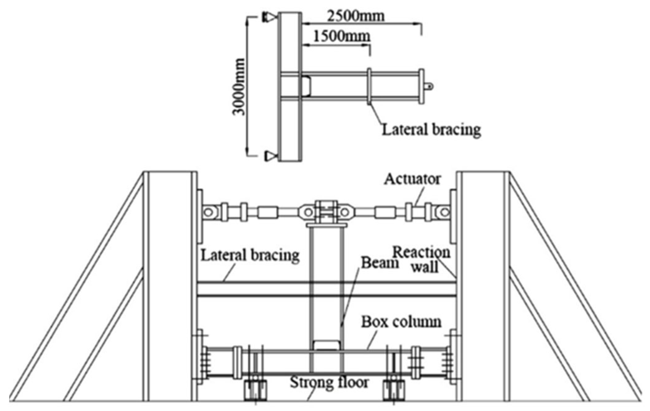
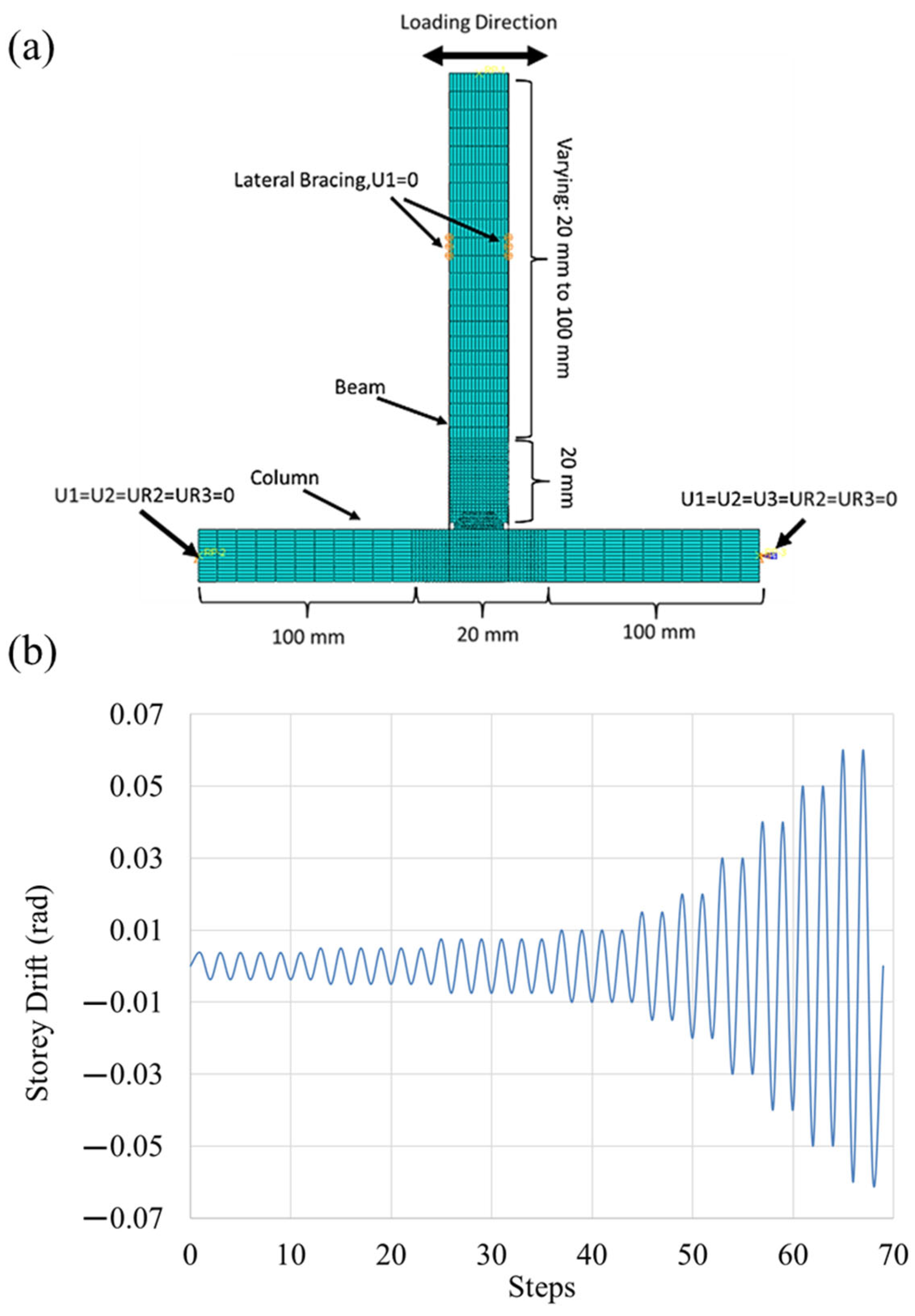
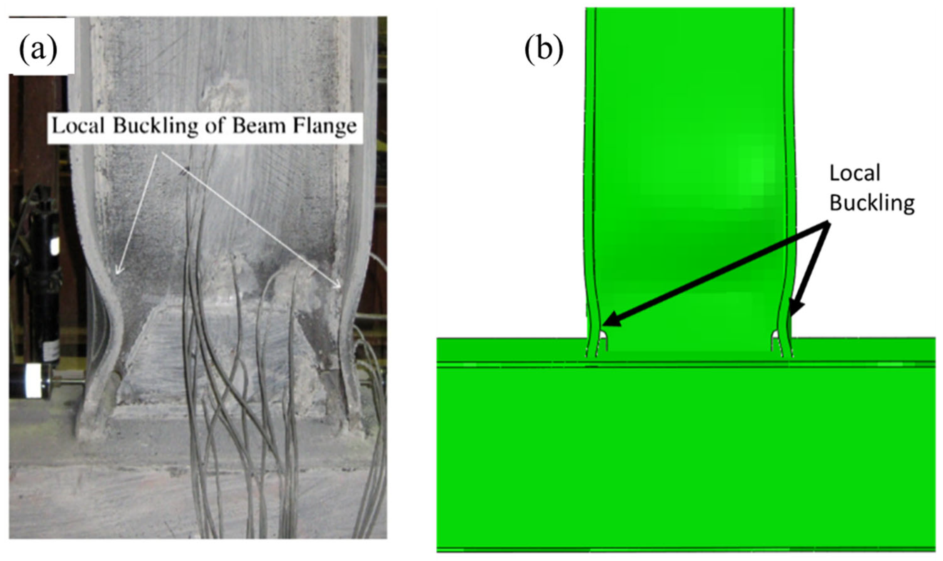
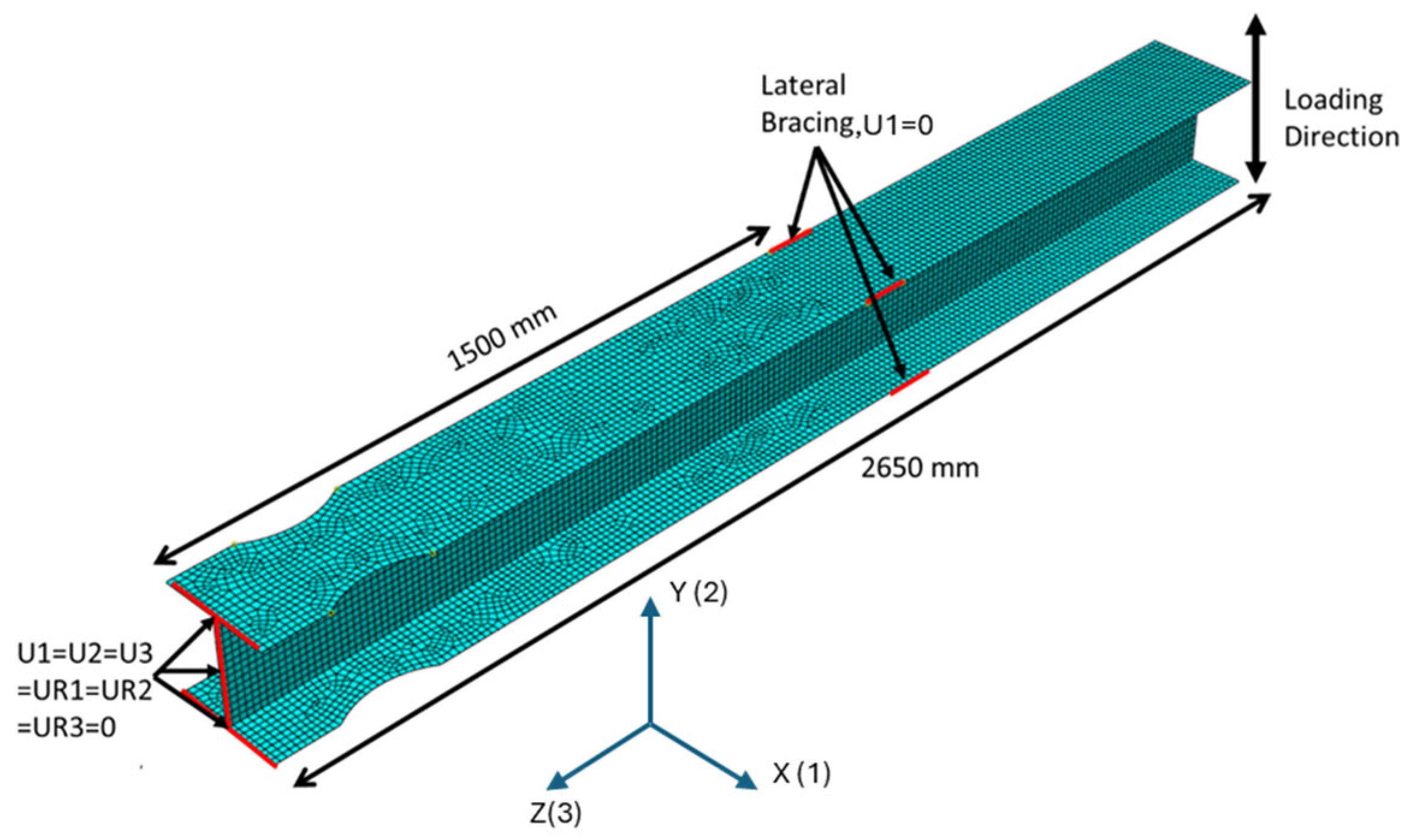
2. Development of FE Model

To develop the database for this research study, the FE model incorporated the specified beam dimensions and radius cut geometries that were built using the general-purpose FE model software ABAQUS [45]. A calibrated FE model was established based on a full-scale beam–column sub-assembly (DC-S) experimentally investigated by [46]. The beam–column sub-assembly, tested by [46], consists of a wide-flange beam section, measuring 330 mm in height and 160 mm in width, welded to a 300 × 300 × 15 mm hollow square column. The thickness of the beam web and flange is 8 mm and 15 mm, respectively. The test setup used in the experiments is illustrated in Figure 1.
To model the beam, column, and shear tab, shell elements were adopted in this study since previous research studies [33,47] showed that shell elements can capture the nonlinear and local buckling behavior of beam–column sub-assemblies. In addition, computational time can be reduced with models developed using shell elements. Four-node shell elements (SR4 [45]) were used to model all components of the beam–column sub-assembly. To reduce computational time, a coarse mesh was used in the areas where plastic deformations were expected to be insignificant, whereas a finer mesh was adopted in the areas where a high intensity of local buckling and plastic deformation was expected. To determine an appropriate mesh size, a trial-and-error approach was followed, iteratively adjusting the mesh until the FE force–displacement curve aligned with the experimental curve. Numerous mesh sizes were considered during this process, and a 20 mm mesh was ultimately identified as the best fit for modeling. It should be noted that when welds are included in such an assembly, a more comprehensive mesh sensitivity analysis may be necessary to ensure the accuracy of stress development in the weld region. A detailed discussion on the impact of mesh size on stress development on the weld can be found in [48]. Figure 2 shows the mesh sizes used in the areas near the welded region and the rest of the model. In addition, Figure 2 also shows the boundary conditions included in the FE model. Similarly, to the experimental work of [46], the suggested AISC 358-16 [13] loading protocol, also shown in Figure 2, was applied in the form of displacement at the tip of the beam. To reduce the computational time, only two cycles for each story drift level were applied.
To capture material nonlinearity, a combined nonlinear isotropic and kinematic strain hardening model, based on the Von Mises yield surface and associated flow rules, was used. The combined hardening material model requires several hardening parameters. To model the isotropic hardening behavior, the model requires the Q and B parameters. Q defines the maximum size that can be reached by the yield surface, and parameter B represents the rate of change in the yield surface as plastic strain increases. To represent kinematic hardening, parameters C and γ are required. C defines the initial kinematic hardening modulus, and γ characterizes the reduction rate of kinematic hardening as plastic strain increases. The parameters used in this study were adopted from [47], which were based on the coupon test conducted by [46]. According to coupon tests [46], the beam flange and web exhibit yield strengths of 252 MPa and 351 MPa, tensile strengths of 399.6 MPa and 482.5 MPa, and elongations of 30.8% and 27.5%, respectively. Later, a few modifications were made to the material parameters, which were based on the suggested values of [47], used in ABAQUS to better capture the deformed shape of the beam section, consistent with the experimental observations. For the beam flange, the Q and B parameters were 48 and 24, respectively, whereas the C and γ parameters were 2400 and 24 [47], respectively. For the beam web, the Q and B parameters were 40 and 20, respectively, while the C and γ parameters were taken as 2400 and 24, respectively.
Another source of nonlinearity in structures arises from geometric nonlinearity, which occurs when large deformations and rotations are expected under severe loading. The analyses enabled the nonlinear geometry (NLGEOM) option in ABAQUS [45] finite element software to account for the nonlinear effects associated with the connection geometry. Figure 2 shows the boundary conditions considered when tip loading is applied in the form of displacement to represent the story drift. The results of the FE models exhibited a good correlation with the experimental beam tip force–story drift relationship, as illustrated in Figure 3. Additionally, the FE models effectively captured the local buckling behavior of the beam flange, closely mirroring the observations from the experimental setup, as depicted in Figure 4, which shows the extruded view for a clear depiction of the buckling observed in the FE model. It should be noted that the welds were not included in the FE simulations, which could contribute to slight discrepancies in the location of the buckled part of the beam flanges.

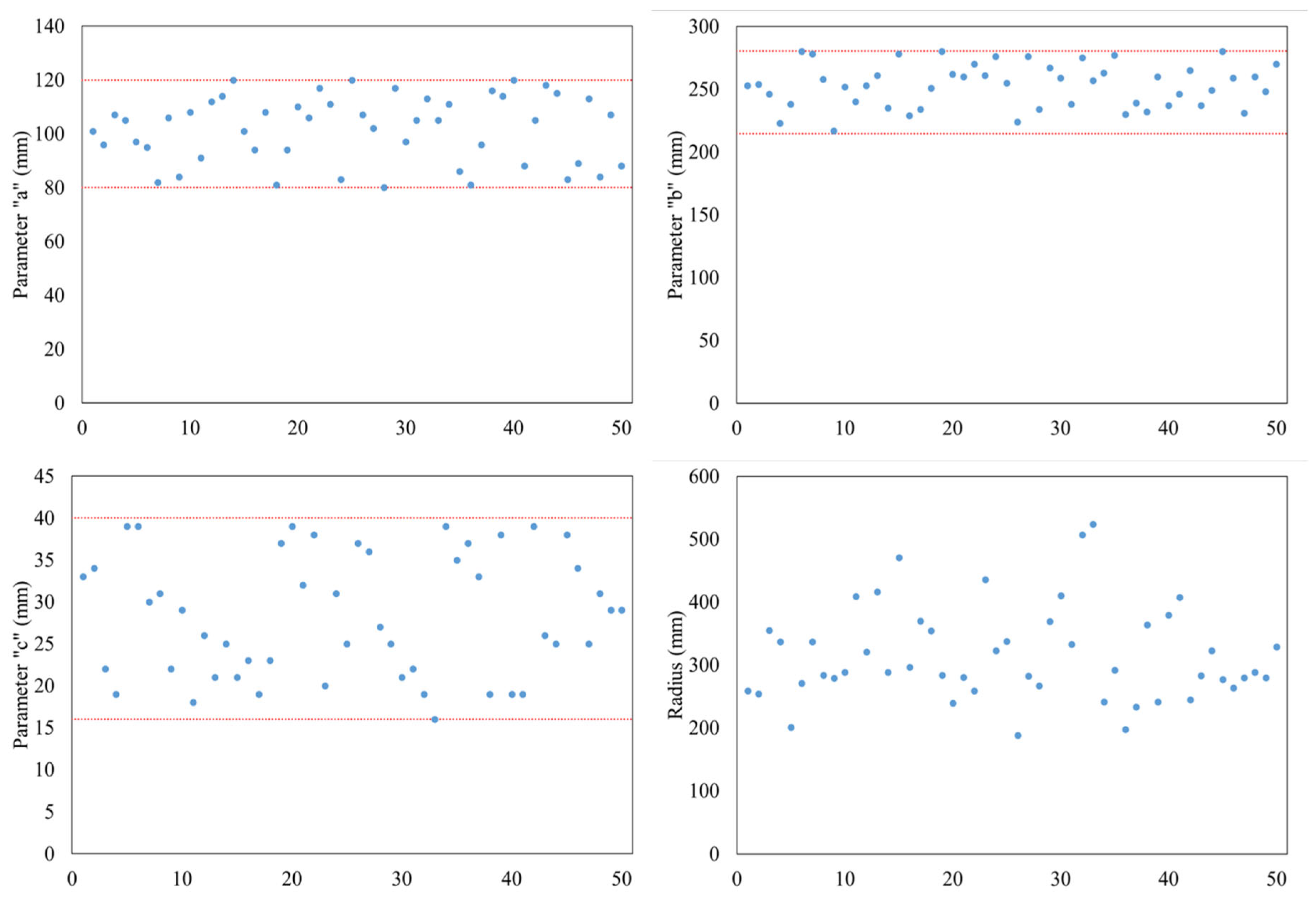
Generation of RBS Connection Database via FE Model

RBS geometric details were developed based on the limitations suggested by AISC 358-22 [44]. The parameter “a” defines the location of the radius cut away from the weld region, parameter “b” specifies the width of the chord of the radius cut, and parameter “c” indicates the depth of the radius cut. Figure 5 illustrates the parameters used in the radius cut along with the limitations outlined in AISC 358-22 [44]. Parameters “a” and “c” are determined based on the width of the beam flanges (bf), while parameter “b” is determined based on the depth “d” of the beam section.
Following the limitation suggested by AISC358-22 [44], ten different beam sections, including the beam tested by [46], were selected. The other nine beam sections were randomly selected from the American wide-flange beams typically used in practice. The beam sections are W10 × 68, W12 × 45, W14 × 48 W16 × 77, W18 × 65, W21 × 50, W24 × 94, W27 × 94, and W30 × 116. For each beam section, 50 random parameter sets were generated, ranging from the lower limit to the upper limit of each parameter. Figure 6 illustrates the parameters selected for a beam section considered in the database.
A script was developed to help speed up the creation of database models with Python. The FE models were simplified to reduce analysis time by omitting the column and only modeling the beam section with the radius cut geometry. The total length of the beam was 2650 mm, and the location of the bracing was 1500 mm away from the welded region. As the goal of this research is to investigate only the impact of RBS geometric details on the moment–rotation behavior of the connection, the shear tab and weld access hole were excluded from the model. To represent the weld, the top and bottom beam flanges, as well as the beam web, were fully restrained, as illustrated in Figure 7. Lateral bracing was applied to prevent lateral–torsional buckling during the analysis. A hex-dominated mesh, depicted in Figure 7, was employed for all beam sections, enabling faster model creation and database development. A seed size of 20 mm was used in the model to create a hex-dominated mesh.
The beams were loaded at the tip up to a displacement corresponding to a 0.04 rad rotation, as suggested by AISC 358-22 [44] which specifies that a connection must achieve a rotation capacity of 0.04 rad for qualification. The loading protocol used for model calibration was also used for the database models with the maximum rotation limited to 0.04 rad. Moreover, for each displacement only one cycle was applied.
A set of Python scripts was developed to extract force–displacement data for all beam sections. To facilitate the data extraction process, a reference point within a geometric set was defined at the free end of the beam models. A tie constraint was then applied between the reference points, the beam flange, and the beam web to ensure the movement of all nodes at the same time. The geometric set allowed for the collection of displacement data along with the corresponding reaction force. Subsequently, the Python script automated the extraction of load–displacement data. Figure 8 illustrates the deformation and equivalent plastic strain (PEEQ) [45] distribution observed in selected FE models from the database and the corresponding backbone curve of moment–rotation.
The relocation of the plastic hinge was successfully achieved across all beam sections with varying radius cut geometries. However, web buckling was observed in deeper beam sections, particularly those with larger radius cuts where the “c” values are significantly large. Additionally, the positioning of the lateral bracing influenced the occurrence of lateral–torsional buckling at both the radius cut section and the beam web. To ensure consistency in data collection, the bracing location was kept the same in all models.

3. Methodology

The methodology for the development of this article is summarized in Figure 9 and is divided into 4 main processes: (1) data development, (2) data handling, (3) model development, and finally (4) model evaluation. Data development is done through ABAQUS [45], while data handling is concerned with the preparation of the data to ensure suitability when used in a machine learning algorithm. Model development focuses on cleaned and adjusted data to develop a generalizable prediction model. Finally, model evaluation assesses the quality of the developed model and explains feature significance using Shapley values.
Once the dataset is generated by the FE model, the dataset is adjusted and cleaned by checking for any missing values. For each unique set of features, the rotation and moment vectors were collected. This led to the development of a structured data frame which is composed of all the features, rotation vectors, and moment vectors. Once the data frame is obtained, a Pearson’s correlation assessment is applied to measure the relationship between each feature and the target variables (those being the moment and rotation vectors). Variables with excessively high correlation above 0.8 are inspected and checked if there exists collinearity using variance inflation factors [49].
Once the variables are finalized, they are scaled using MinMaxScaler to ensure that all the values are on a uniform range, thus reducing the impact of varying feature magnitudes on the model since some models such as ANN are sensitive to feature scaling [50,51]. The approach used in MinMaxScaler is illustrated in Equation (1).
X s c a l e d = X X m i n X m a x X m i n r m a x r m i n + r m i n
where
  • X: the original data point.
  • Xmin: the minimum value in the feature (column).
  • Xmax: the maximum value in the feature (column).
  • Xscaled: the scaled value of X.
  • rmin: the desired minimum range of the transformed data (default is 0).
  • rmax: the desired maximum range of the transformed data (default is 0).
During data handling, Q-Q plots were obtained in order to assess the distribution of each feature. The results revealed that features have a normal distribution except for tf, tw, and bf, as shown in Figure 10. These three features are section properties, and they have fixed dimensions. After scaling, the rotation and moment vectors were united into a matrix to form a single variable output. The dataset is split into an 80% training dataset and 20% testing dataset, which is later used for the 5-fold cross-validation procedure.
Moving to model development, Artificial Neural Networks (ANN), Random Forest (RF), Support Vector Machines (SVM), Gradient Boosting (GB) and Ridge Regression (RR) were employed to predict the desired outputs, consecutively applying the same modeling principles to each model such as scaling, hyperparameter tuning using grid search, and cross-validation.
The forward propagation process in ANN involves computing the weighted sums of inputs followed by using activation functions to introduce nonlinearity. The learning process is optimized using backpropagation, which minimizes the prediction error by adjusting the weights through gradient descent. The weight update rule is governed by Equation (2) [52]:
W = η L W
where
  • W is the weight update.
  • η is the learning rate.
  • L W is the gradient loss function with respect to the weights.
This approach enables the ANN to learn complex relationships between input features and target variables, making it suitable for predicting the moment–rotation backbone curve of Reduced Beam Section (RBS) connections under cyclic loading.
To ensure the regressor’s success and the generalizability of the final output, cross-validation and hyperparameter optimization were applied. Cross-validation was conducted using a 5-fold approach where the dataset is split into five folds and trained on four of the folds, while the fifth fold is used as a validation fold. This process is repeated until all folds are used as training and validation folds.
Hyperparameter tuning was conducted using GridSearchCV of the scikit-learn library of Python [53]. Grid search relies on exhaustively searching through hyperparameter values and evaluating their performance using cross-validation. Hyperparameter tuning has significant effects on model performance, and a systematic tuning procedure must be followed [54]. The final model consisted of three hidden layers with 128, 64, and 32 neurons, using ReLU activation functions and a linear output layer. Training was conducted using the Nadam optimizer, with a batch size of 32 and an initial epoch limit of 1000. To enhance convergence and generalization, early stopping with a patience of 30 epochs and a learning rate scheduler (ReduceLROnPlateau, factor = 0.5, patience = 10) were incorporated. These hyperparameters were selected based on iterative experimentation and validation performance.
To further evaluate the predictive capabilities of the developed Artificial Neural Network (ANN) model, a comparative analysis was conducted against several widely used machine learning algorithms, including Random Forest, Gradient Boosting, Support Vector Regression (SVR), Ridge Regression, and Polynomial Ridge Regression. The performance of each model was assessed using standard regression metrics—the Mean Absolute Error (MAE), mean squared error (MSE), and Coefficient of Determination (R2). Table 3 summarizes the comparative results, highlighting the ANN model’s superior accuracy and reliability in capturing the complex nonlinear behavior of Reduced Beam Section (RBS) connections under cyclic loading.
In the model evaluation phase, models were evaluated using the following metrics:
  • Root Mean Squared Error (RMSE): This metric checks the standard deviation of prediction errors.
R M S E = 1 n i = 1 n ( y i y ^ i ) 2
  • Mean Absolute Error (MAE): This metric measures the average magnitude of prediction errors.
M A E = 1 n i = 1 n | y i y ^ i | 2
  • R-squared (R2): This metric measures the variance within the model for the desired output.
R 2 = 1 i = 1 n ( y i y ^ i ) 2 i = 1 n ( y i y ¯ ) 2
  • Explained Variance Score: This metric measures the extent to which the developed model captures data variability.
E V S = 1 V a r ( y y ^ i ) V a r ( y )
where
  • y i : actual value.
  • y ^ i : predicted value.
  • y ¯ : mean.
  • n : number of observations.
  • V a r ( y   y ^ ) : variance of predictions.
  • V a r ( y ) : variance of actual results.
Structural engineering often involves the development of sophisticated computational models to simulate the behavior of structures under various loading conditions, environmental factors, and material properties. However, understanding the models and disclosing insights into the models require model explainability. To explain models, Shapley numbers are used in this study. The Shapley number (or Shapley value) is a concept from cooperative game theory that quantifies the fair contribution of each player (or feature) in a collaborative setting [55]. It is widely used in machine learning, particularly in XAI, to interpret the contribution of each feature in a predictive model [56].
The Shapley value framework, which originated in game theory, offers a principled approach to feature importance estimation by assigning a unique value to each feature that represents its marginal contribution to the model’s output, considering all possible combinations of the other features [57]. One key benefit of Shapley values is their ability to handle complex, nonlinear relationships between the input features and the model output, which are common in structural engineering applications [58].
The Shapley value, introduced by Lloyd S. Shapley in 1953, is a solution concept in cooperative game theory that fairly allocates the total payoff of a coalition among its individual players based on their marginal contributions [59]. It provides a unique method for distributing gains among participants in a game with transferable utility, ensuring fairness.
Mathematically, let a predictive model obtained from a structural system be represented as a cooperative game (N, v) where
  • N is the set of all structural elements.
  • v(S) is a system performance function (dependent variable) for a subset S of elements.
  • The Shapley value for an element i is given by Equation (7) [59].
ϕ i v = S N { i } S N S 1 ! N ! v S { i } v S
  • S represents a subset of structural elements excluding element i.
  • v S { i } v S quantifies the marginal contribution of element i to system performance.
  • The weighting factor ensures that the contribution is averaged over all possible permutations of element additions.

4. Results and Discussion

Prior to the development of machine learning models, the dataset was rigorously examined to ensure completeness and reliability. Several critical parameters influencing the behavior of Reduced Beam Section (RBS) connections commonly implemented in seismic-resistant steel structures were analyzed. Notably, the dataset was found to contain no missing values, indicating that all measurements for each variable were properly recorded. This characteristic is particularly significant as incomplete data may lead to erroneous conclusions or necessitate estimation methods that could introduce bias.
To quantify the relationships between various parameters, Pearson’s correlation coefficient was employed, as illustrated in Table 4. This statistical measure evaluates linear dependence between variables, where values approaching +1 indicate strong positive correlation, −1 signifies strong negative correlation, and 0 denotes no linear relationship. The analysis revealed several key findings:
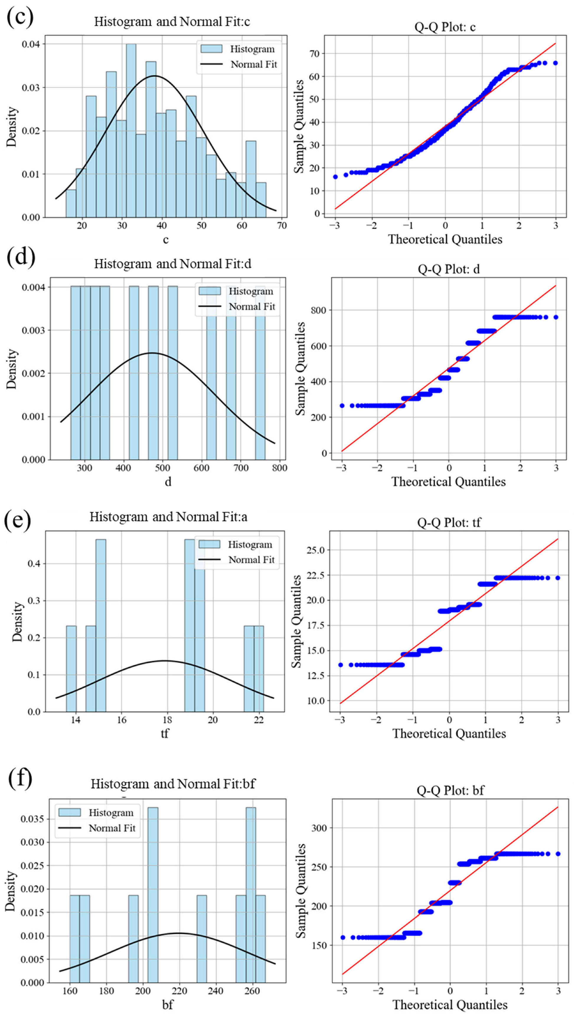
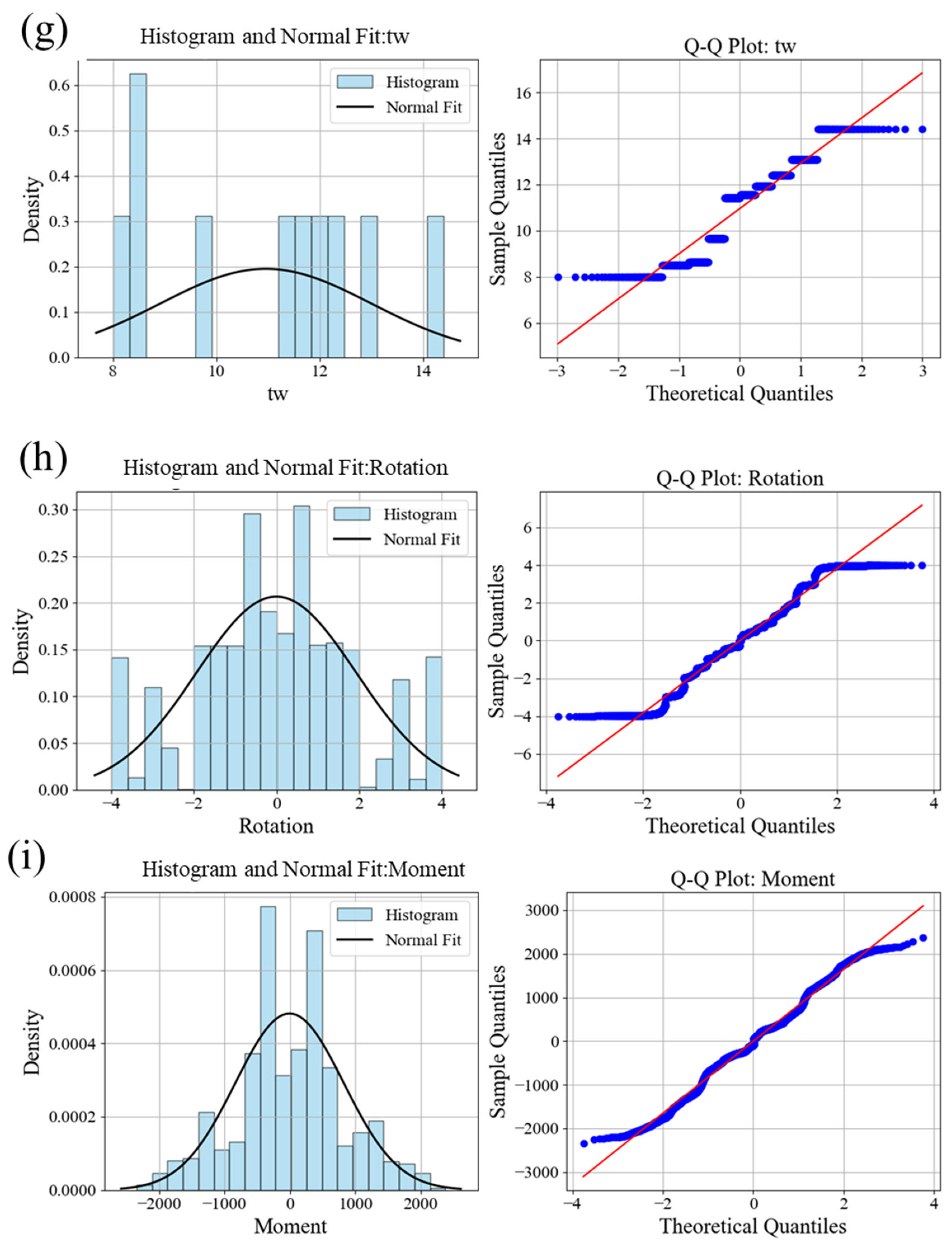
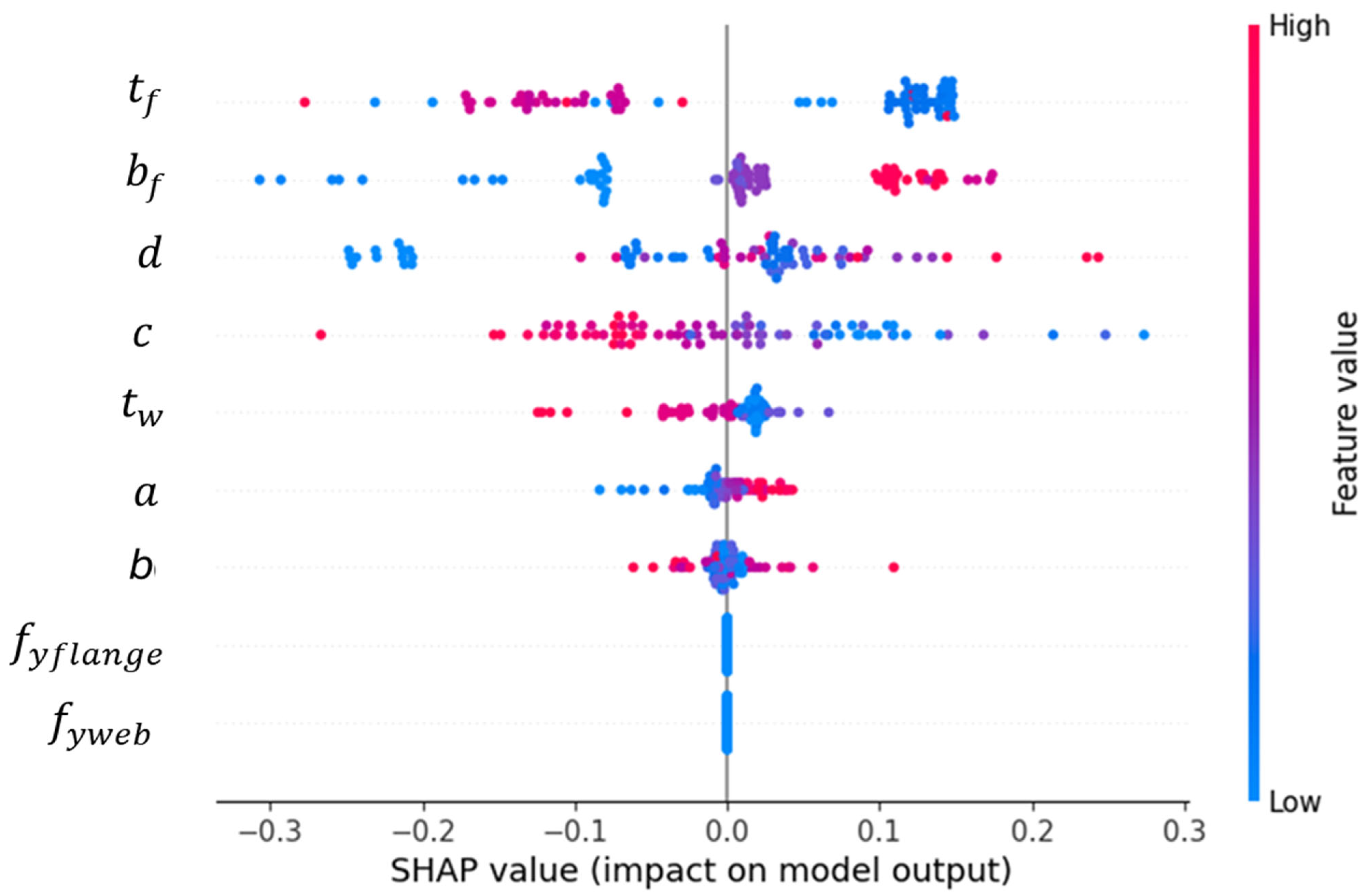
  • Material strength parameters (Yield_web and Yield_flange) demonstrated a negligible correlation (r = 0.1073), suggesting that variations in steel strength did not significantly influence connection behavior within this dataset.
  • Flange thickness (tf) and width (bf) exhibited weak positive correlations (r = 0.2457 and 0.1992, respectively), indicating only marginal improvements in performance with increased dimensions.
  • Beam depth “d” showed the strongest influence among geometric parameters (r = 0.3142), implying that deeper sections provide enhanced bending resistance in RBS connections.
  • Among RBS cut parameters, variable b (r = 0.3004) displayed the most substantial correlation, likely reflecting the importance of reduced section length in controlling connection behavior.
  • Among all RBS cut parameters, the maximum r obtained is 0.3142, which indicates a weak linear relationship between corresponding variables. This also indicates a low possibility of multicollinearity since the Pearson correlation coefficient can also be used as an indicator of multicollinearity [49].
The ANN model demonstrated exceptional predictive capability among all models applied, achieving an R2 value of 99.964% with relatively low error metrics (RMSE = 6.201; MAE = 2.73). These results, summarized in Table 4, suggest that the model successfully captured complex, nonlinear relationships that conventional statistical methods might overlook. The predictive capability of the machine learning model is further demonstrated in Figure 11, which compares the model’s predictions against actual experimental or simulated results for combined rotation and moment behavior. The close alignment between predicted (X) and actual (dashed line) values across the full range of rotational demands (±4%) and moment capacities (±1500 kN-m) validates the model’s accuracy in capturing the nonlinear hysteretic response of RBS connections. Additionally, it can be inferred from the figure that the model successfully replicates the characteristic pinching and stiffness degradation of RBS connections under cyclic loading, evidenced by the overlapping predicted and actual curves. This confirms its ability to simulate energy dissipation and plastic hinge formation—critical for seismic performance. At extreme rotations (±3–4%), where FE model simulations often diverge due to material nonlinearities, the ML model maintains high fidelity. This suggests superior generalization to rare but critical failure scenarios compared to traditional methods. Anecdotally, minor deviations (e.g., slight underprediction at peak positive moments) are systematic rather than random, indicating potential for refinement by incorporating localized buckling effects in future training data.
Furthermore, the figure corroborates the earlier correlation analysis: while material properties (Yield_web/flange) showed negligible influence in linear terms, the model’s accurate hysteresis prediction confirms that it has learned their nonlinear role in plastic deformation. The dominance of geometric parameters (d, b) is reflected in the model’s precise tracking of moment capacity (y-axis) and rotation capacity (x-axis), both of which are geometrically driven.
The findings indicate that ML approaches may significantly enhance structural engineering practices by achieving the following:
1
Accelerating the design process through rapid performance predictions, particularly for
  • Code compliance checks (e.g., AISC358-22 rotation limits).
  • Parametric studies optimizing RBS cut dimensions (a, b, c).
2
Enabling the optimization of critical parameters such as beam depth and RBS cut length.
3
Potentially reducing material costs through more efficient designs.
4
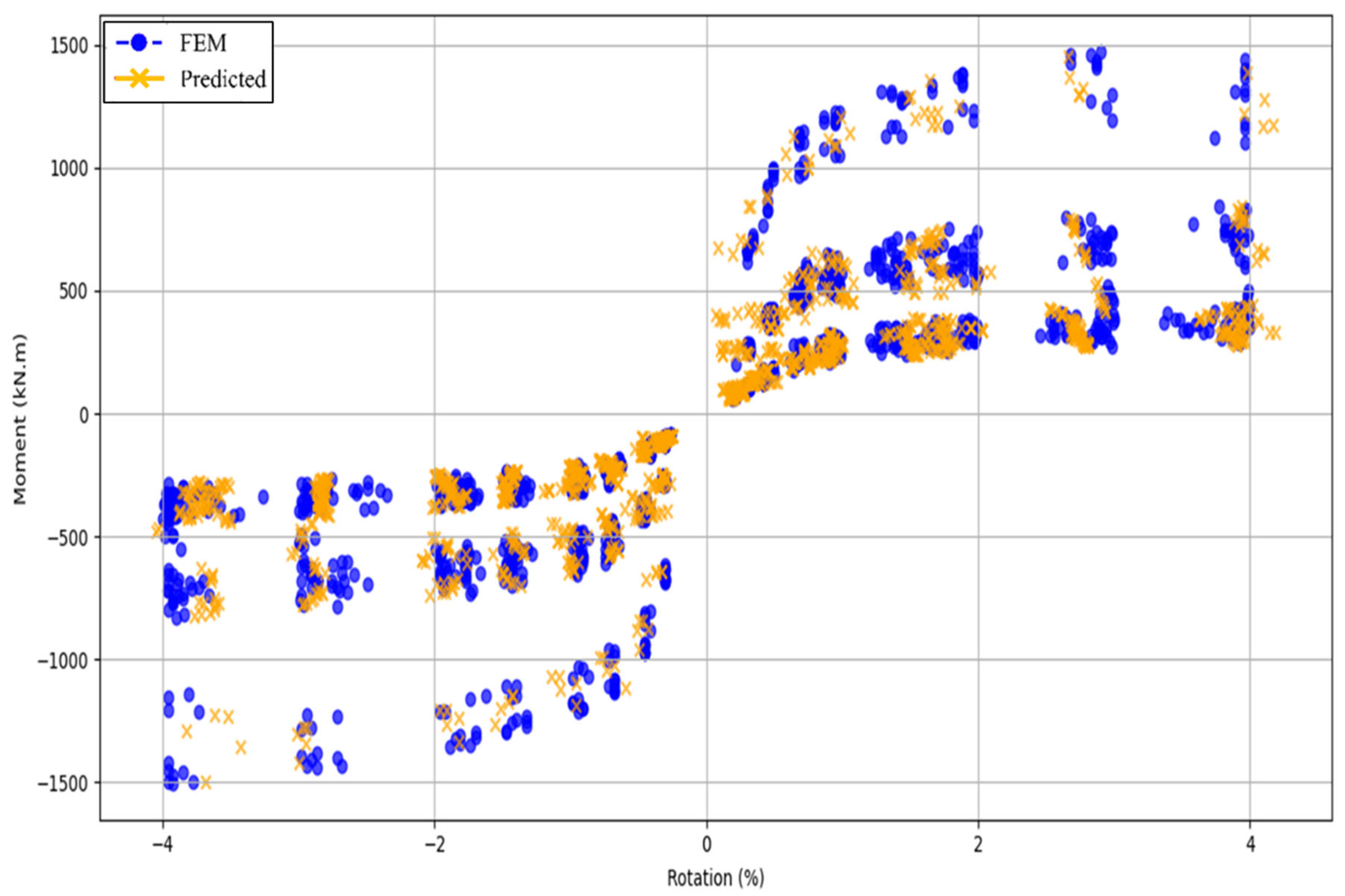
The tight error envelope (±500 kN-m at extremes) supports its use in reliability-based design, where quantifying uncertainty is essential.
As shown in Figure 12, the ANN effectively predicts the backbone curves of various beam sections. The deformation patterns under cyclic loading further validate the occurrence of plastic hinge buckling, which corresponds to the load drops observed in the backbone curves for certain beam sections. Minor discrepancies in rotation levels between the FE model and the machine learning predictions are noted likely due to the material models employed; however, these discrepancies remain within acceptable limits.
The SHAP values obtained from the analysis showed the clarification of the model inputs and outputs, as can be seen in Figure 13. tf, bf, d, and c have a wider spread of SHAP values, indicating that they have a significant influence on the model predictions. Their SHAP values range from negative to positive in a long range, meaning that their effect varies based on the feature values. Wide SHAP distribution and their values (both high and low) can either increase or decrease model predictions in mixed ways. A close look at the results also reveals that fyflange and fyweb have the least effect on the model output. These features have SHAP values clustered around zero, showing that they do not significantly influence model predictions. Likely, their contribution to the model’s decision-making is minimal.
The mean SHAP values provide valuable insights into the behavior of RBS connections. The discussion on moment capacity should be divided into two key aspects. First, cross-sectional properties play a significant role in determining moment capacity. As the beam depth “d” increases, the lever arm between the flanges becomes larger, which in turn increases the moment capacity, as expected. Additionally, flange thickness “tf ” and beam flange width “bf” are crucial, since the beam flanges provide a larger amount of moment resistance. In contrast, web thickness “tw” contributes the least. These findings are aligned with the SHAP values given in Figure 13. It should be noted that since one material type is utilized in the FE models, the contribution of flange and web yield does not have an impact on the model compared to other parameters. Second, aside from cross-sectional properties, the moment capacity is affected by the parameters of the radius cut geometry. The graph of the mean SHAP values indicates that parameter “c” is the most critical parameter within the parameters, used to define radius cut, as it significantly affects moment capacity and plastic hinge formation. An increase in “c” results in a reduced flange width which subsequently lowers the moment capacity and shifts hinge formation away from the weld region. These findings align with the numerical research conducted by [20,60] and the FE models developed and analyzed in this research study. Parameters “a” and “b” have the least impact on behavior. These findings are also aligned with the following design equations provided by AISC 358-22 [44].
Z R B S = Z b 2 c t b f ( d t b f )
where Zb is the plastic section modulus of the beam, tf is the thickness of the flange, d is the depth of the beam, and c is the maximum length on the radius. bf is the width of the beam flange, embedded in Zb. According to this equation, a large value of “c” will lead to a lower plastic section modulus which in turn results in a lower probable maximum moment at the plastic hinge which can be calculated as follows:
M p r = C p r R y F y Z e
where Ze = ZRBS, Cpr is factor representing the maximum connection strength, Fy is the yield stress of the beam member, and Ry is the ratio of the expected yield stress to the specified minimum yield stress.
In summary, among all models evaluated, the Artificial Neural Network (ANN) emerged as the optimal predictor for RBS connection backbone curves under cyclic loading, demonstrating superior accuracy and reliability. It achieved the lowest prediction error (MAE = 2.73) and highest goodness of fit (R2 = 99.964%) of any model, notably outperforming the other high-performing algorithms in this study (Random Forest: MAE 2.93, R2 99.816%; Gradient Boosting: MAE 3.21, R2 99.807%; Support Vector Regression: MAE 3.08, R2 99.669%). This exceptional performance was matched by excellent generalization: the ANN maintained consistent accuracy on independent test data and effectively captured the complex nonlinear relationships inherent in the RBS dataset [61]. Moreover, rigorous cross-validation and hyperparameter tuning (GridSearchCV) were employed to prevent overfitting, ensuring that the model’s predictive capability remained robust when confronted with unseen scenarios [62]. Equally important, the inclusion of SHAP-based explainability imparted the model with a high degree of transparency, revealing that the ANN’s predictions are governed by the same key geometric factors (most notably the RBS cut depth) known to influence connection behavior. This alignment of the model’s logic with the established physical behavior of RBS geometries bolsters confidence in its predictions. Together, these attributes not only validate the choice of the ANN as the predictive tool in this study but also highlight the promise of integrating explainable AI into structural engineering practice—paving the way for more transparent, high-fidelity predictive models to enhance the future design and analysis of resilient structures.

5. Conclusions

This study aimed to develop several ML models to predict the moment rotation backbone curve of RBS connections subjected to simulated cyclic loading, in accordance with current design guidelines. The FE model analysis results from ten wide-flange beams with varying geometric configurations were utilized. A dataset comprising 500 beam sections with different RBS parameters was used to train and validate the ANN model through 5-fold cross-validation and hyperparameter tuning.
Among all ML models the ANN model demonstrated high accuracy with a 99.964% R2 in predicting the backbone curves of beam sections, regardless of the presence of local buckling at the plastic hinge region. Furthermore, XAI methods with SHAP (SHapley Additive exPlanations) values provided insights into model interpretability, revealing trends that are consistent with code-prescribed design equations for RBS connections. Among the input parameters, the “c” parameter—governing the depth of the radius cut—was identified as the most influential factor. In addition to the “c” parameter, flange thickness and beam depth were also found to be critical factors, validating the findings from previous experimental studies.
While these findings are promising, this study presents several limitations, particularly from a machine learning perspective, that merit further exploration. First, the FE model was created for a limited number of randomly selected wide-flange beams, and incorporating a broader range of beam types could have improved the model’s generalizability. Second, the material model used in the analysis represents only a subset of structural steel properties. Given the variability in steel behavior, integrating a wider spectrum of material characteristics into the ML model would likely enhance its predictive capability. Third, the lateral bracing locations were based on a specific experimental setup, which restricts the model’s applicability to other configurations. Additionally, the total beam length, which significantly influences buckling behavior in combination with bracing location, presents another constraint. Calibrated FE models along with experimental tests are necessary to validate the model’s predictions, particularly at higher failure rotations exceeding 4%. In addition, the contribution of weld and panel zones to moment–rotation behavior should be included in model generation to increase generalizability. Finally, to ensure broader applicability, the model should be tested on unconventional geometries, such as those with varying span-to-depth ratios.
From a computational standpoint, the model was trained exclusively on numerically generated data. While this approach offers consistency and scalability, it may not capture real-world uncertainties present in experimental conditions. Moreover, although SHAP values offered valuable interpretability, they remain post hoc and sensitive to model architecture and feature distribution, highlighting a need for more robust explainability strategies.
Future work should explore hybrid modeling approaches that combine ML predictions with physics-informed constraints to improve generalization and physical consistency. Additionally, expanding the training dataset to include experimental data, exploring uncertainty quantification methods (e.g., Bayesian networks), and validating the model on nonstandard geometries or alternative structural typologies such as bolted or composite joints could significantly improve model reliability. The real-time integration of such explainable AI models into design workflows or structural health monitoring platforms also presents an exciting opportunity for advancing data-driven structural engineering.

Author Contributions

Methodology, E.T. and F.U.; Software, S.E.-Z.; Resources, S.E.-Z.; Data curation, E.T.; Writing—original draft, E.T., M.Y.C., F.U. and S.E.-Z.; Writing—review & editing, F.U.; Visualization, M.Y.C. All authors have read and agreed to the published version of the manuscript.

Funding

This research received no external funding.

Data Availability Statement

The original contributions presented in the study are included in the article, further inquiries can be directed to the corresponding author/s.

Conflicts of Interest

The authors declare no conflict of interest.

References

  1. Federal Emergency Management Agency. A Policy Guide to Steel Moment-Frame Construction (FEMA 354). SAC Joint Venture. 2000. Available online: https://www.nehrp.gov/pdf/fema354.pdf (accessed on 10 May 2025).
  2. Roeder, C.W.; Venture, S.A.C.J. State of the Art Report on Connection Performance. Federal Emergency Management Agency (FEMA) Bulletin, (355D). 2000. Available online: https://www.nehrp.gov/pdf/fema355d.pdf (accessed on 2 June 2025).
  3. Engelhardt, M.D.; Sabol, T.A. Seismic-resistant steel moment connections: Developments since the 1994 Northridge earthquake. Prog. Struct. Eng. Mater. 1997, 1, 68–77. [Google Scholar] [CrossRef]
  4. Uang, C.-M.; Yu, Q.-S.; Kent, Y.; Noel, S.; Gross, J. Cyclic Testing of Steel Moment Connections Rehabilitated with RBS or Welded Haunch. J. Struct. Eng. 2000, 126, 57–68. [Google Scholar] [CrossRef]
  5. Chen, S.-J.; Chao, Y.C. Effect of composite action on seismic performance of steel moment connections with reduced beam sections. J. Constr. Steel Res. 2001, 57, 417–434. [Google Scholar] [CrossRef]
  6. Gilton, C.S.; Uang, C.-M. Cyclic Response and Design Recommendations of Weak-Axis Reduced Beam Section Moment Connections. J. Struct. Eng. 2002, 128, 452–463. [Google Scholar] [CrossRef]
  7. Lee, C.-H.; Jeon, S.-W.; Kim, J.-H.; Uang, C.-M. Effects of Panel Zone Strength and Beam Web Connection Method on Seismic Performance of Reduced Beam Section Steel Moment Connections. J. Struct. Eng. 2005, 131, 1854–1865. [Google Scholar] [CrossRef]
  8. Lee, C.-H.; Kim, J.-H. Seismic design of reduced beam section steel moment connections with bolted web attachment. J. Constr. Steel Res. 2007, 63, 522–531. [Google Scholar] [CrossRef]
  9. Pachoumis, D.T.; Galoussis, E.G.; Kalfas, C.N.; Christitsas, A.D. Reduced beam section moment connections subjected to cyclic loading: Experimental analysis and FEM simulation. Eng. Struct. 2009, 31, 216–223. [Google Scholar] [CrossRef]
  10. Ohsaki, M.; Tagawa, H.; Pan, P. Shape optimization of reduced beam section under cyclic loads. J. Constr. Steel Res. 2009, 65, 1511–1519. [Google Scholar] [CrossRef]
  11. Pachoumis, D.T.; Galoussis, E.G.; Kalfas, C.N.; Efthimiou, I.Z. Cyclic performance of steel moment-resisting connections with reduced beam sections—Experimental analysis and finite element model simulation. Eng. Struct. 2010, 32, 2683–2692. [Google Scholar] [CrossRef]
  12. Han, S.W.; Moon, K.-H.; Hwang, S.-H.; Stojadinovic, B. Rotation capacities of reduced beam section with bolted web (RBS-B) connections. J. Constr. Steel Res. 2012, 70, 256–263. [Google Scholar] [CrossRef]
  13. American Institute of Steel Construction. AISC 358-16: Seismic Provisions for Structural Steel Buildings; American Institute of Steel Construction: Chicago, IL, USA, 2016. [Google Scholar]
  14. Sofias, C.E.; Kalfas, C.N.; Pachoumis, D.T. Experimental and FEM analysis of reduced beam section moment endplate connections under cyclic loading. Eng. Struct. 2014, 59, 320–329. [Google Scholar] [CrossRef]
  15. Oh, K.; Lee, K.; Chen, L.; Hong, S.-B.; Yang, Y. Seismic performance evaluation of weak axis column-tree moment connections with reduced beam section. J. Constr. Steel Res. 2015, 105, 28–38. [Google Scholar] [CrossRef]
  16. Li, R.; Samali, B.; Tao, Z.; Kamrul Hassan, M. Cyclic behaviour of composite joints with reduced beam sections. Eng. Struct. 2017, 136, 329–344. [Google Scholar] [CrossRef]
  17. Morshedi, M.A.; Dolatshahi, K.M.; Maleki, S. Double reduced beam section connection. J. Constr. Steel Res. 2017, 138, 283–297. [Google Scholar] [CrossRef]
  18. Sophianopoulos, D.S.; Deri, A.E. Steel beam-to-column RBS connections with European profiles: I. Static optimization. J. Constr. Steel Res. 2017, 139, 101–109. [Google Scholar] [CrossRef]
  19. Liu, C.; Wu, J.; Xie, L. Seismic performance of buckling-restrained reduced beam section connection for steel frames. J. Constr. Steel Res. 2021, 181, 106622. [Google Scholar] [CrossRef]
  20. Horton, T.A.; Hajirasouliha, I.; Davison, B.; Ozdemir, Z. More efficient design of reduced beam sections (RBS) for maximum seismic performance. J. Constr. Steel Res. 2021, 183, 106728. [Google Scholar] [CrossRef]
  21. Horton, T.A.; Hajirasouliha, I.; Davison, B.; Ozdemir, Z.; Abuzayed, I. Development of more accurate cyclic hysteretic models to represent RBS connections. Eng. Struct. 2021, 245, 112899. [Google Scholar] [CrossRef]
  22. Özkılıç, Y.O.; Bozkurt, M.B. Numerical validation on novel replaceable reduced beam section connections for moment-resisting frames. Structures 2023, 50, 63–79. [Google Scholar] [CrossRef]
  23. Yao, Y.; Zhou, L.; Huang, H.; Chen, Z.; Ye, Y. Cyclic performance of novel composite beam-to-column connections with reduced beam section fuse elements. Structures 2023, 50, 842–858. [Google Scholar] [CrossRef]
  24. Thai, H.-T. Machine learning for structural engineering: A state-of-the-art review. Structures 2022, 38, 448–491. [Google Scholar] [CrossRef]
  25. Almasabha, G.; Alshboul, O.; Shehadeh, A.; Almuflih, A.S. Machine Learning Algorithm for Shear Strength Prediction of Short Links for Steel Buildings. Buildings 2022, 12, 775. [Google Scholar] [CrossRef]
  26. Avci-Karatas, C. Application of Machine Learning in Prediction of Shear Capacity of Headed Steel Studs in Steel–Concrete Composite Structures. Int. J. Steel Struct. 2022, 22, 539–556. [Google Scholar] [CrossRef]
  27. Dabiri, H.; Rahimzadeh, K.; Kheyroddin, A. A comparison of machine learning- and regression-based models for predicting ductility ratio of RC beam-column joints. Structures 2022, 37, 69–81. [Google Scholar] [CrossRef]
  28. De Oliveira, V.M.; De Carvalho, A.S.; Rossi, A.; Hosseinpour, M.; Sharifi, Y.; Martins, C.H. Data-driven design approach for the lateral-distortional buckling in steel-concrete composite cellular beams using machine learning models. Structures 2024, 61, 106018. [Google Scholar] [CrossRef]
  29. Dissanayake, M.; Nguyen, H.; Poologanathan, K.; Perampalam, G.; Upasiri, I.; Rajanayagam, H.; Suntharalingam, T. Prediction of shear capacity of steel channel sections using machine learning algorithms. Thin-Walled Struct. 2022, 175, 109152. [Google Scholar] [CrossRef]
  30. Liu, J.; Li, S.; Guo, J.; Xue, S.; Chen, S.; Wang, L.; Zhou, Y.; Luo, T.X. Machine learning (ML) based models for predicting the ultimate bending moment resistance of high strength steel welded I-section beam under bending. Thin-Walled Struct. 2023, 191, 111051. [Google Scholar] [CrossRef]
  31. Marie, H.S.; Abu El-Hassan, K.; Almetwally, E.M.; A. El-Mandouh, M. Joint shear strength prediction of beam-column connections using machine learning via experimental results. Case Stud. Constr. Mater. 2022, 17, e01463. [Google Scholar] [CrossRef]
  32. Rahman, J.; Ahmed, K.S.; Khan, N.I.; Islam, K.; Mangalathu, S. Data-driven shear strength prediction of steel fiber reinforced concrete beams using machine learning approach. Eng. Struct. 2021, 233, 111743. [Google Scholar] [CrossRef]
  33. Horton, T.A.; Hajirasouliha, I.; Davison, B.; Ozdemir, Z. Accurate prediction of cyclic hysteresis behaviour of RBS connections using Deep Learning Neural Networks. Eng. Struct. 2021, 247, 113156. [Google Scholar] [CrossRef]
  34. Guzmán-Torres, J.A.; Domínguez-Mota, F.J.; Martínez-Molina, W.; Naser, M.Z.; Tinoco-Guerrero, G.; Tinoco-Ruíz, J.G. Damage detection on steel-reinforced concrete produced by corrosion via YOLOv3: A detailed guide. Front. Built Environ. 2023, 9, 1144606. [Google Scholar] [CrossRef]
  35. Hsiao, C.-H.; Kumar, K.; Rathje, E. Explainable AI models for predicting liquefaction-induced lateral spreading (Version 1). arXiv 2024. [Google Scholar] [CrossRef]
  36. Janouskova, K.; Rigotti, M.; Giurgiu, I.; Malossi, C. Model-Assisted Labeling via Explainability for Visual Inspection of Civil Infrastructures (No. arXiv:2209.11159). arXiv 2022. [Google Scholar] [CrossRef]
  37. Zhang, T.; Vaccaro, M.; Zaghi, A.E. Application of neural networks to the prediction of the compressive capacity of corroded steel plates. Front. Built Environ. 2023, 9, 1156760. [Google Scholar] [CrossRef]
  38. Mangalathu, S.; Hwang, S.-H.; Jeon, J.-S. Failure mode and effects analysis of RC members based on machine-learning-based SHapley Additive exPlanations (SHAP) approach. Eng. Struct. 2020, 219, 110927. [Google Scholar] [CrossRef]
  39. Wakjira, T.G. Plastic hinge length of rectangular RC columns using ensemble machine learning model. Eng. Struct. 2021, 244, 112808. [Google Scholar] [CrossRef]
  40. Angelucci, G.; Quaranta, G.; Mollaioli, F.; Kunnath, S.K. Interpretable machine learning models for displacement demand prediction in reinforced concrete buildings under pulse-like earthquakes. J. Build. Eng. 2024, 95, 110124. [Google Scholar] [CrossRef]
  41. Zhu, Y.; Taffese, W.Z.; Chen, G. Enhancing FRP-concrete interface bearing capacity prediction with explainable machine learning: A feature engineering approach and SHAP analysis. Eng. Struct. 2024, 319, 118831. [Google Scholar] [CrossRef]
  42. Shahmansouri, A.A.; Jafari, A.; Bengar, H.A.; Zhou, Y.; Taciroglu, E. A scaling-based generalizable integrated ML-mechanics model for lateral response of self-centering walls. Eng. Struct. 2025, 336, 120326. [Google Scholar] [CrossRef]
  43. Fryer, D.; Strümke, I.; Nguyen, H. Shapley values for feature selection: The good, the bad, and the axioms. IEEE Access 2021, 9, 144352–144360. [Google Scholar] [CrossRef]
  44. American Institute of Steel Construction. AISC 358-22: Prequalified Connections for Special and Intermediate Steel Moment Frames for Seismic Applications; American Institute of Steel Construction: Chicago, IL, USA, 2022. [Google Scholar]
  45. Dassault Systèmes Simulia Corp. ABAQUS User’s, Theory, and Scripting Manuals; Dassault Systèmes: Johnston, RI, USA, 2024. [Google Scholar]
  46. Saneei Nia, Z.; Ghassemieh, M.; Mazroi, A. WUF-W connection performance to box column subjected to uniaxial and biaxial loading. J. Constr. Steel Res. 2013, 88, 90–108. [Google Scholar] [CrossRef]
  47. Asil Gharebaghi, S.; Fami Tafreshi, R.; Fanaie, N.; Sepasgozar Sarkhosh, O. Optimization of the Double Reduced Beam Section (DRBS) Connection. Int. J. Steel Struct. 2021, 21, 1346–1369. [Google Scholar] [CrossRef]
  48. Chen, F.; Liu, X.; Zhang, H.; Luo, Y.; Lu, N.; Liu, Y.; Xiao, X. Assessment of fatigue crack propagation and lifetime of double-sided U-rib welds considering welding residual stress relaxation. Ocean. Eng. 2025, 332, 121400. [Google Scholar] [CrossRef]
  49. Shrestha, N. Detecting multicollinearity in regression analysis. Am. J. Appl. Math. Stat. 2020, 8, 39–42. [Google Scholar] [CrossRef]
  50. Mining, W.I.D. Data mining: Concepts and techniques. Morgan Kaufinann 2006, 10, 4. [Google Scholar]
  51. Nielsen, M.A. Neural Networks and Deep Learning; Determination Press: San Francisco, CA, USA, 2015; Volume 25. [Google Scholar]
  52. Goodfellow, I.; Bengio, Y.; Courville, A.; Bengio, Y. Deep Learning; MIT Press: Cambridge, UK, 2016; Volume 1. [Google Scholar]
  53. Pedregosa, F.; Varoquaux, G.; Gramfort, A.; Michel, V.; Thirion, B.; Grisel, O.; Blondel, M.; Prettenhofer, P.; Weiss, R.; Dubourg, V. Scikit-learn: Machine learning in Python. J. Mach. Learn. Res. 2011, 12, 2825–2830. [Google Scholar]
  54. Sonmez, R.; Uysal, F. Discussion of “Artificial Intelligence and Parametric Construction Cost Estimate Modeling: State-of-the-Art Review” by Haytham H. Elmousalami. J. Constr. Eng. Manag. 2021, 147, 07021001. [Google Scholar] [CrossRef]
  55. Hart, S. Shapley Value. In Game Theory (210–216); Springer: Berlin/Heidelberg, Germany, 1989. [Google Scholar]
  56. Cicek, E.; Akin, M.; Uysal, F.; Topcu Aytas, R. Comparison of traffic accident injury severity prediction models with explainable machine learning. Transp. Lett. 2023, 15, 1043–1054. [Google Scholar] [CrossRef]
  57. Li, X.; Zhou, Y.; Dvornek, N.C.; Gu, Y.; Ventola, P.; Duncan, J.S. Efficient Shapley explanation for features importance estimation under uncertainty. In Proceedings of the Medical Image Computing and Computer Assisted Intervention–MICCAI 2020: 23rd International Conference, Lima, Peru, 4–8 October 2020; Proceedings, Part I 23. Springer International Publishing: Cham, Switzerland, 2020; pp. 792–801. [Google Scholar]
  58. Movsessian, A.; Cava, D.G.; Tcherniak, D. Interpretable Machine Learning in Damage Detection Using Shapley Additive Explanations. ASCE-ASME J. Risk Uncertain. Eng. Syst. Part B Mech. Eng. 2022, 8, 021101. [Google Scholar] [CrossRef]
  59. Shapley, L.S. Stochastic Games. Proc. Natl. Acad. Sci. USA 1953, 39, 1095–1100. [Google Scholar] [CrossRef]
  60. Al-Saeedi, S.M.A.A.; Lu, L.; Al-Ansi, O.Z.Y.; Ali, S. Hysteretic Behavior Study on the RBS Connection of H-Shape Columns with Middle-Flanges or Wide-Flange H-Shape Beams. Buildings 2025, 15, 147. [Google Scholar] [CrossRef]
  61. Al-Massri, G.; Ghanem, H.; Khatib, J.; El-Zahab, S.; Elkordi, A. The Effect of Adding Banana Fibers on the Physical and Mechanical Properties of Mortar for Paving Block Applications. Ceramics 2024, 7, 1533–1553. [Google Scholar] [CrossRef]
  62. El-Mir, A.; El-Zahab, S. Assessment of the Compressive Strength of Self-Consolidating Concrete Subjected to Freeze-Thaw Cycles Using Ultrasonic Pulse Velocity Method. Russ. J. Nondestruct. Test. 2022, 58, 108–117. [Google Scholar] [CrossRef]
Figure 1. Experimental setup reprinted with permission from [46].
Buildings 15 02307 g001
Figure 2. (a) Mesh size used in calibration model and boundary conditions. (b) Loading protocol.
Buildings 15 02307 g002
Figure 3. Comparison of story drift vs. force at tip beam for FE model and experiment adapted from [46].
Buildings 15 02307 g003
Figure 4. (a) Observed damage in experiment reprinted with permission from ([46]). (b) Observed damage in FE model.
Buildings 15 02307 g004
Figure 5. Radius cut geometric parameters and limitations.
Buildings 15 02307 g005
Figure 6. Sample of randomly selected parameters for radius cut geometry.
Buildings 15 02307 g006
Figure 7. FE model boundary conditions for simplified analysis.
Buildings 15 02307 g007
Figure 8. Sample FE analysis result and corresponding backbone curve with deformed shape for W21 × 50.
Buildings 15 02307 g008
Figure 9. Methodology of this study.
Buildings 15 02307 g009
Figure 10. Distribution of input parameters and Q-Q plots for (a) parameter ‘a’, (b) parameter ‘b’, (c) parameter ‘c’, (d) beam depth, (e) flange thickness (tf), (f) flange width (bf), (g) web thickness (tw), (h) rotation, and (i) moment.
Buildings 15 02307 g010aBuildings 15 02307 g010bBuildings 15 02307 g010c
Figure 11. Moment–rotation (FE model vs. predicted).
Buildings 15 02307 g011
Figure 12. Moment–rotation prediction for non-buckled and buckled beams.
Buildings 15 02307 g012
Figure 13. SHAP value distribution.
Buildings 15 02307 g013
Table 1. Literature summary of RBS studies.
ResearchMethod *Summary
Uang et al. [4]EInvestigated the impact of RBS and welded haunches on the cyclic behavior of steel moment connections
Chen and Chao [5]EDemonstrated that a beam-to-column connection with RBS could achieve an average plastic rotation of 0.045 rad
Gilton and Uang [6]E and NInvestigated the cyclic behavior of weak-axis RBS moment connections
Lee et al. [7]EInvestigated the seismic behavior of RBS steel moment connections
Lee and Kim [8]EInvestigated RBS moment connections with bolted webs
Pachoumis et al. [9]E and NInvestigated the application of RBS connections to European steel beam profiles
Ohsaki et al. [10]NOptimization of RBS details
Han et al. [12] Investigated the rotation capacity of RBS with bolted webs
Sofias et al. [14]EInvestigated the behavior of RBS moment connections with extended bolted end plates
Oh et al. [15]EInvestigated weak-axis column-tree moment connections featuring RBS and tapered beams
Li et al. [16]EInvestigated the cyclic performance of composite joints with RBS connected to concrete-filled tubular (CFT) columns
Morshedi et al. [17]NIntroduced an innovative steel moment connection, named the Double Reduced Beam Section (DRBS) connection
Sophianopoulos and Deri [18]NDeveloped an optimization methodology for RBS connections using European steel profiles
Liu et al. [19]E and NProposed a buckling-restrained RBS connection
Horton et al. [20]NIdentified the key parameters influencing the seismic performance of RBS connections
Horton et al. [21]NDeveloped a database of modified Ibarra–Krawinkler (mIK) models for American wide-flange beams with RBS connections
Ozkilic and Bozkurt [22]NProposed a replaceable RBS connection
Yao et al. [23]E and NDeveloped a novel Reduced Beam Section (RBS) steel composite frame beam
* E: experimental; N: numerical.
Table 3. Comparative performance of machine learning models for predicting RBS moment–rotation backbone curves.
ModelMAEMSER2 Score
ANN2.7338.45299.964%
Random Forest2.931531.52399.816%
SVR3.078355.46499.669%
Gradient Boosting3.214533.1499.807%
PolyRidge (deg = 2)5.721176.93699.543%
Ridge19.774604.9796.489%
Table 4. Summary of missing values and Pearson’s correlation coefficients.
Metric Missing ValuesPearson’s Correlation CoefficientsCommentary
INPUT VARIABLESYield web (fy web)Yield strength of the web 00.1073Negligible correlation, suggesting independent material behavior.
Yield Flange (fy flange)Yield strength of the flange 00.1073
tfFlange thickness 00.2457Weak influence; thicker flanges slightly improve performance.
bfFlange width 00.1992Minimal impact, indicating width is less critical than depth.
dOverall depth of the beam cross-section00.3142Strongest geometric influence; deeper beams enhance stiffness/strength.
twWeb thickness00.1532Marginal effect, implying web buckling is not dominant.
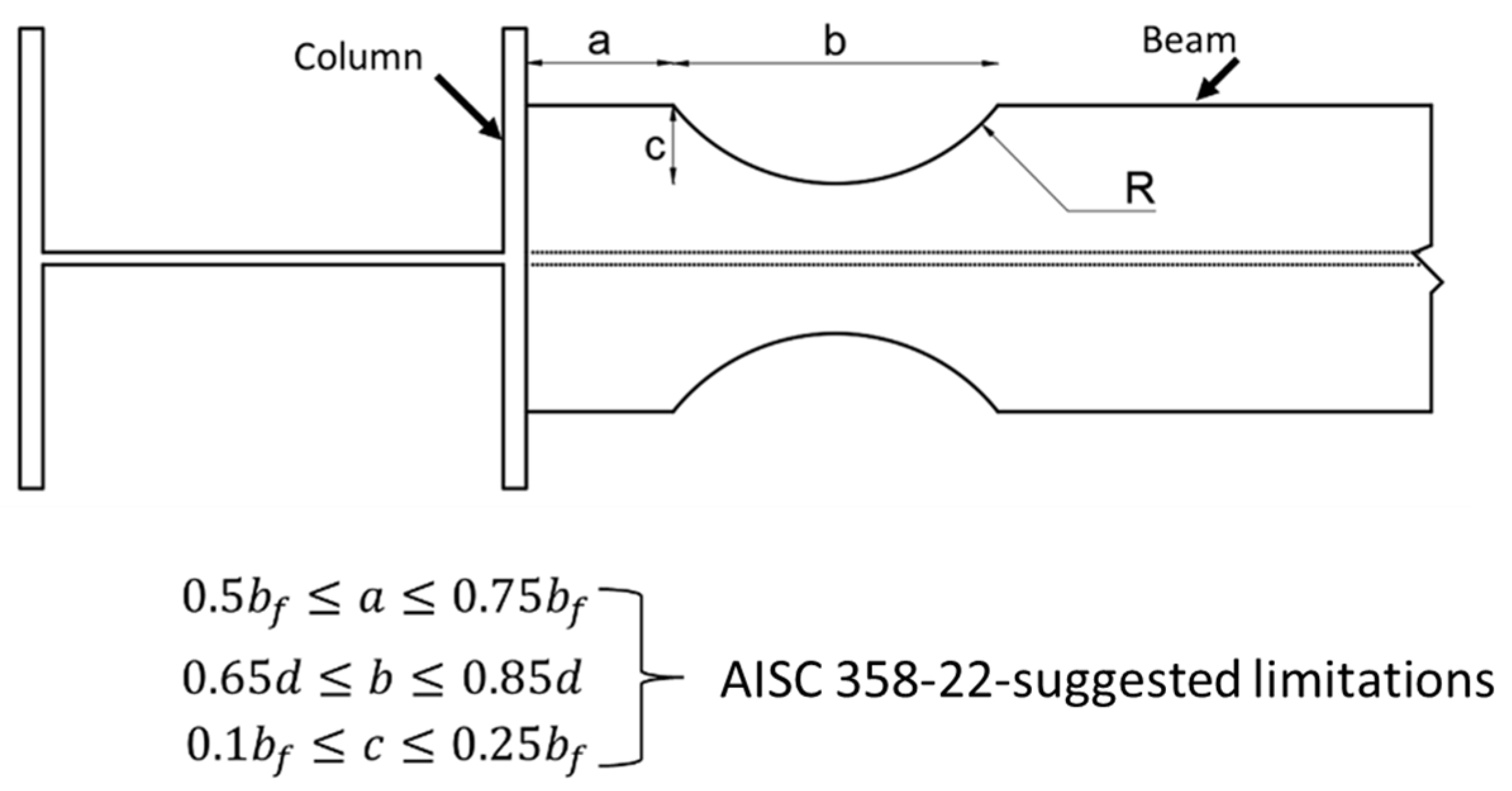
aDistance from the column face to the start of the flange cut (start of the RBS)00.1790Parameter b has the highest impact, suggesting cut length is crucial.
bLength of the flange reduction zone (where the flange is reduced in width)00.3004
cDepth of the flange cut (the maximum vertical depth removed from the flange edge)00.0745
TARGET VARIABLESRotationRotational deformation values (%) forming a vector of 16 points for the backbone curve0---
MomentCorresponding flexural moment values (kNm), also a 16-point vector forming the backbone curve0---
Disclaimer/Publisher’s Note: The statements, opinions and data contained in all publications are solely those of the individual author(s) and contributor(s) and not of MDPI and/or the editor(s). MDPI and/or the editor(s) disclaim responsibility for any injury to people or property resulting from any ideas, methods, instructions or products referred to in the content.

