
Application of Curtain Grouting for Seepage Control in the Dongzhuang Dam: A 3D Fracture Network Modeling Approach
Abstract
1. Introduction
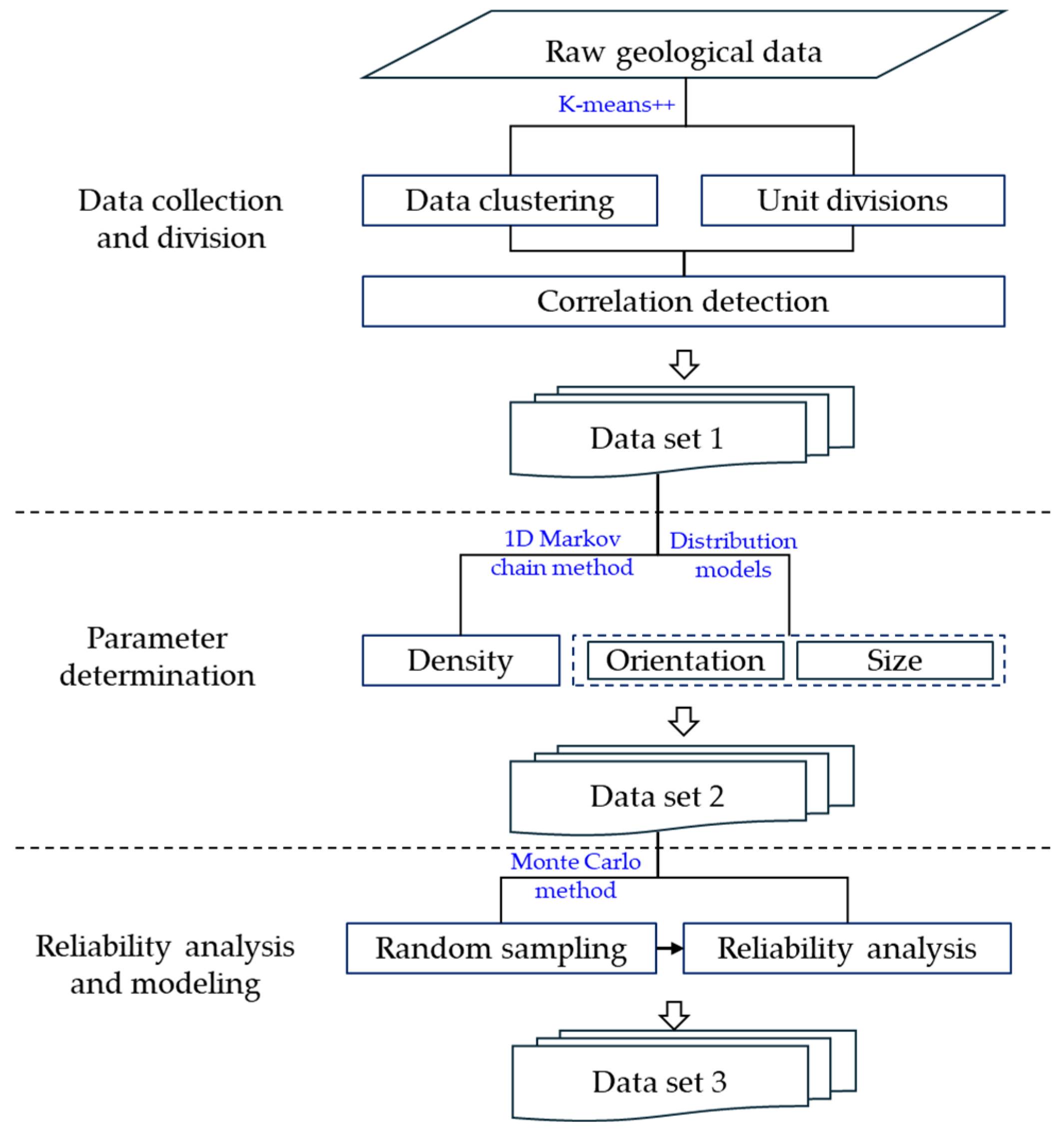
2. Methodology
2.1. First-Order Markov Chain Property Test for Fracture Data Processing
2.2. Methods for Parameter Determination
2.2.1. One-Dimensional Markov Chain Model
- (1)
- The transition probabilities between different density attributes of adjacent units are calculated using the following equation [27]:where Xi represents the geological unit at location i, and Sk denotes the attribute of the geological unit. The probability of transitioning from attribute k in the geological unit to attribute q is obtained by raising the one-step transition probability matrix to the power of N − i.
- (2)
- The transition of fracture density attributes from a known unit to its adjacent unit. The process repeats until the fracture density of all predicted units is determined according to the following [27]:where u represents a uniformly distributed random number generated in the interval [0, 1].
2.2.2. Distribution Model of Fracture Orientation and Size
2.3. Evaluation
2.3.1. Performance of Fracture Density Prediction
- (1)
- Coefficient of determination, R2
- (2)
- Accuracy matric, ACC
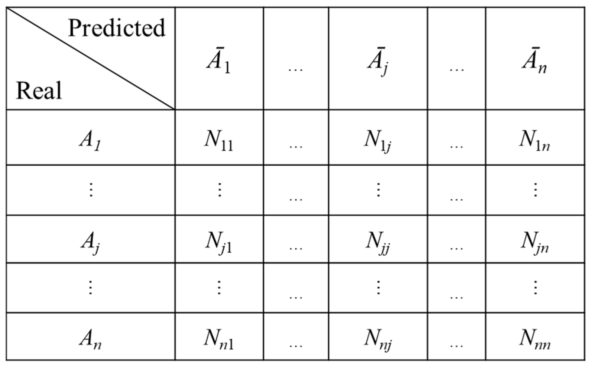
- (3)
- Confusion matrix
2.3.2. Reliability Analysis
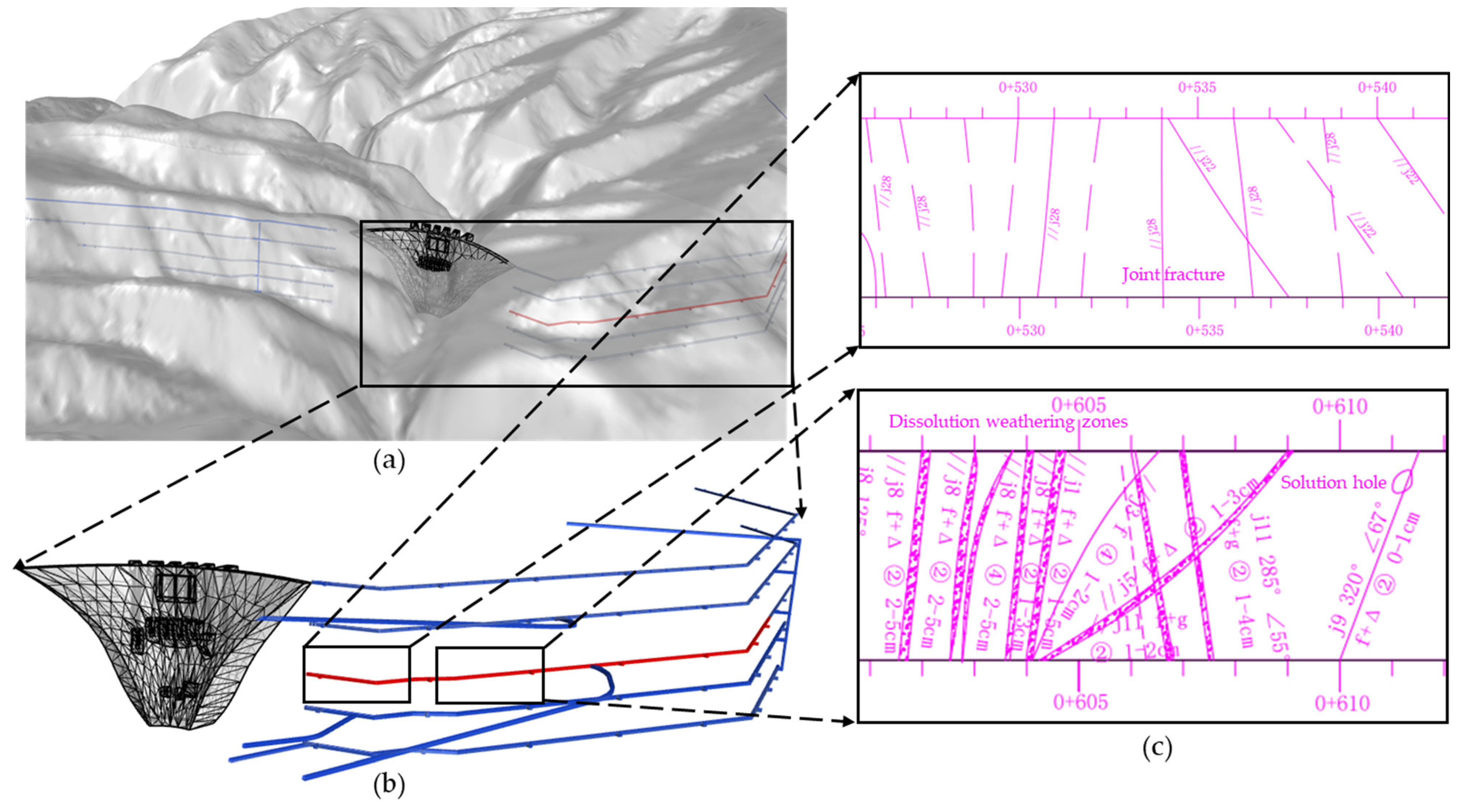
3. Simulation
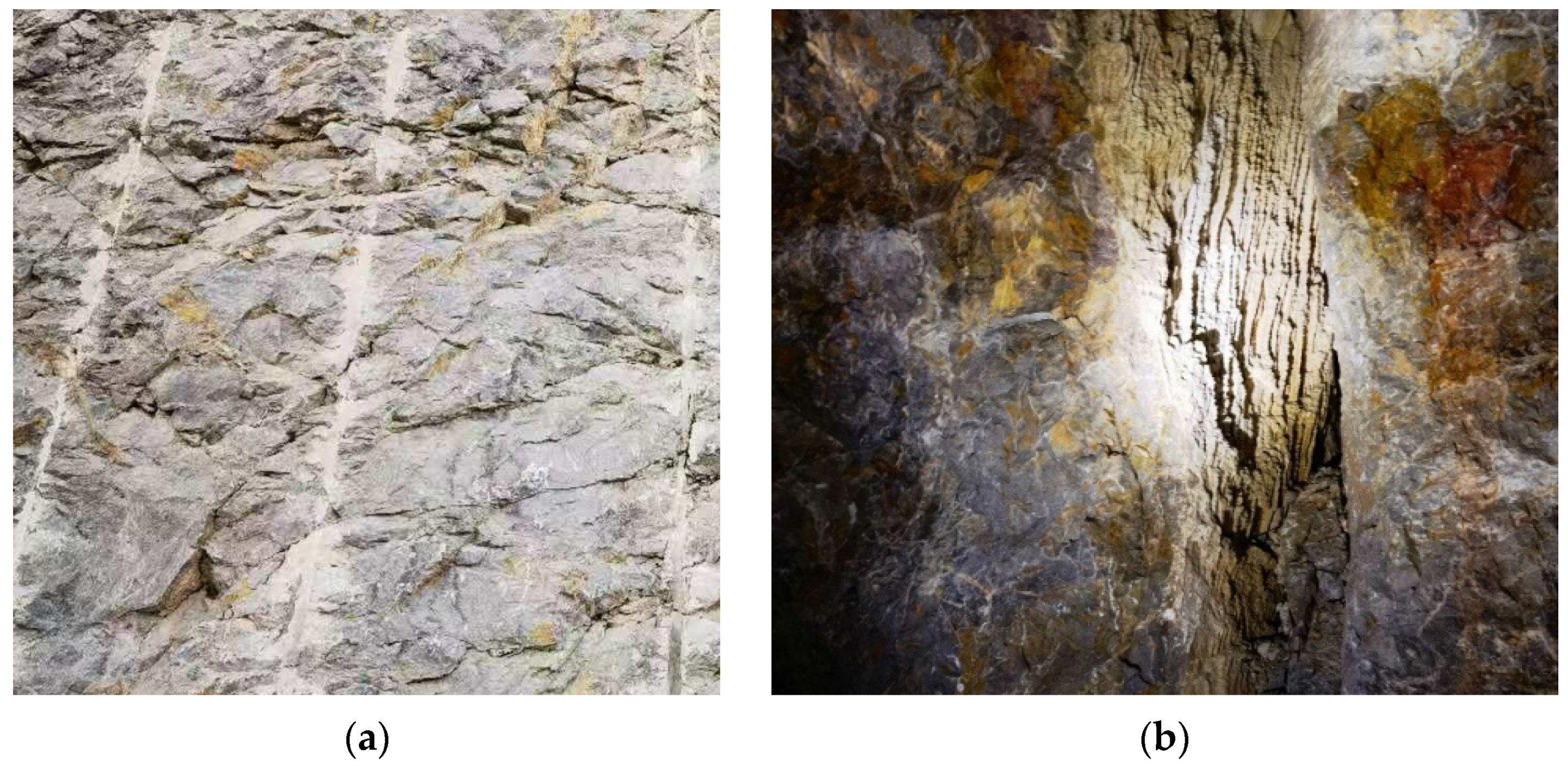
3.1. Background
3.2. Data Division
3.3. Parameter Determinations
- (1)
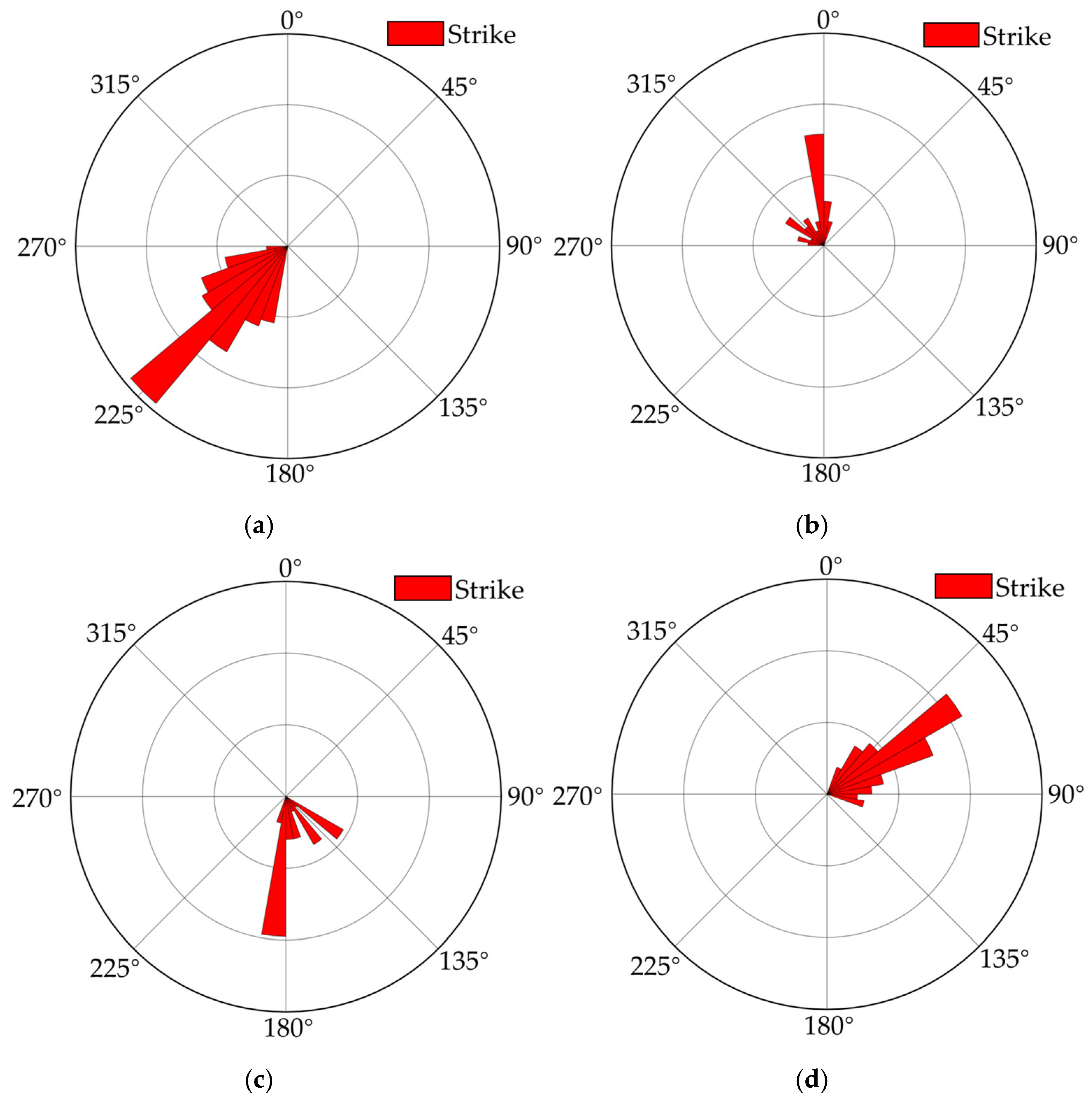
- Fracture orientations
- (2)
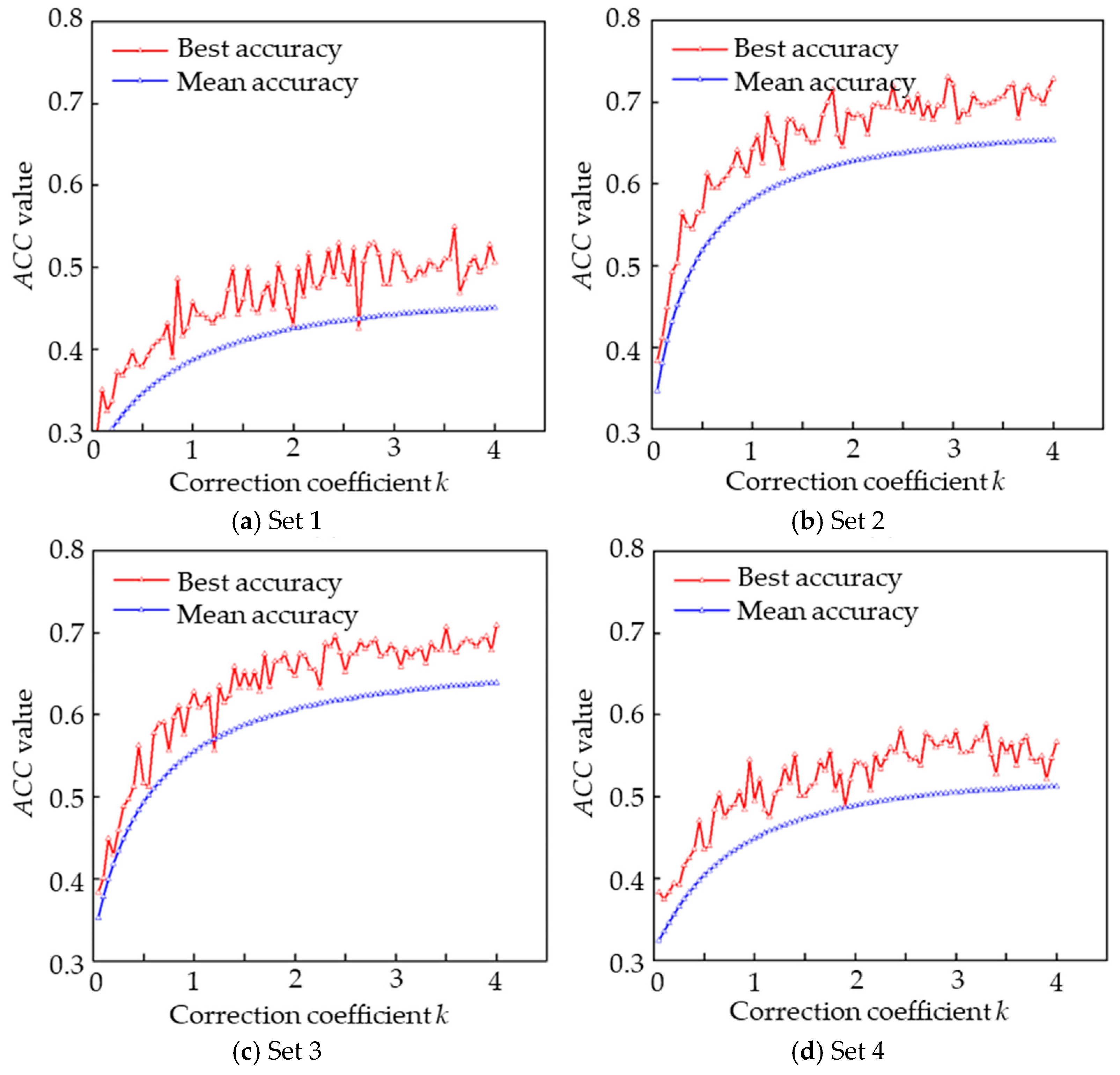
- Fracture density
- (3)
- Performances of predictions for fracture parameters
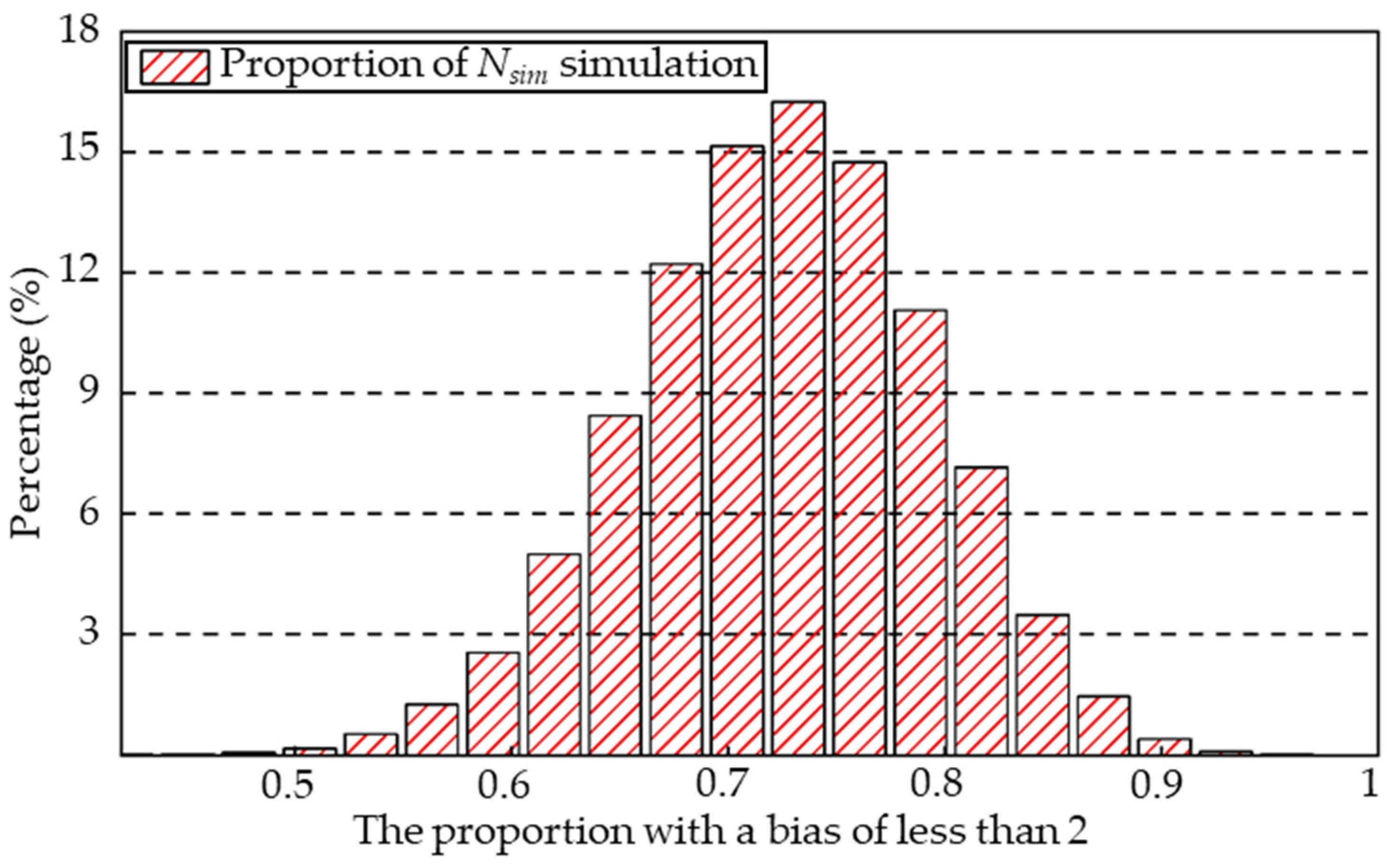
3.4. Reliability Analysis of Simulation Results
3.5. Fracture Diameter
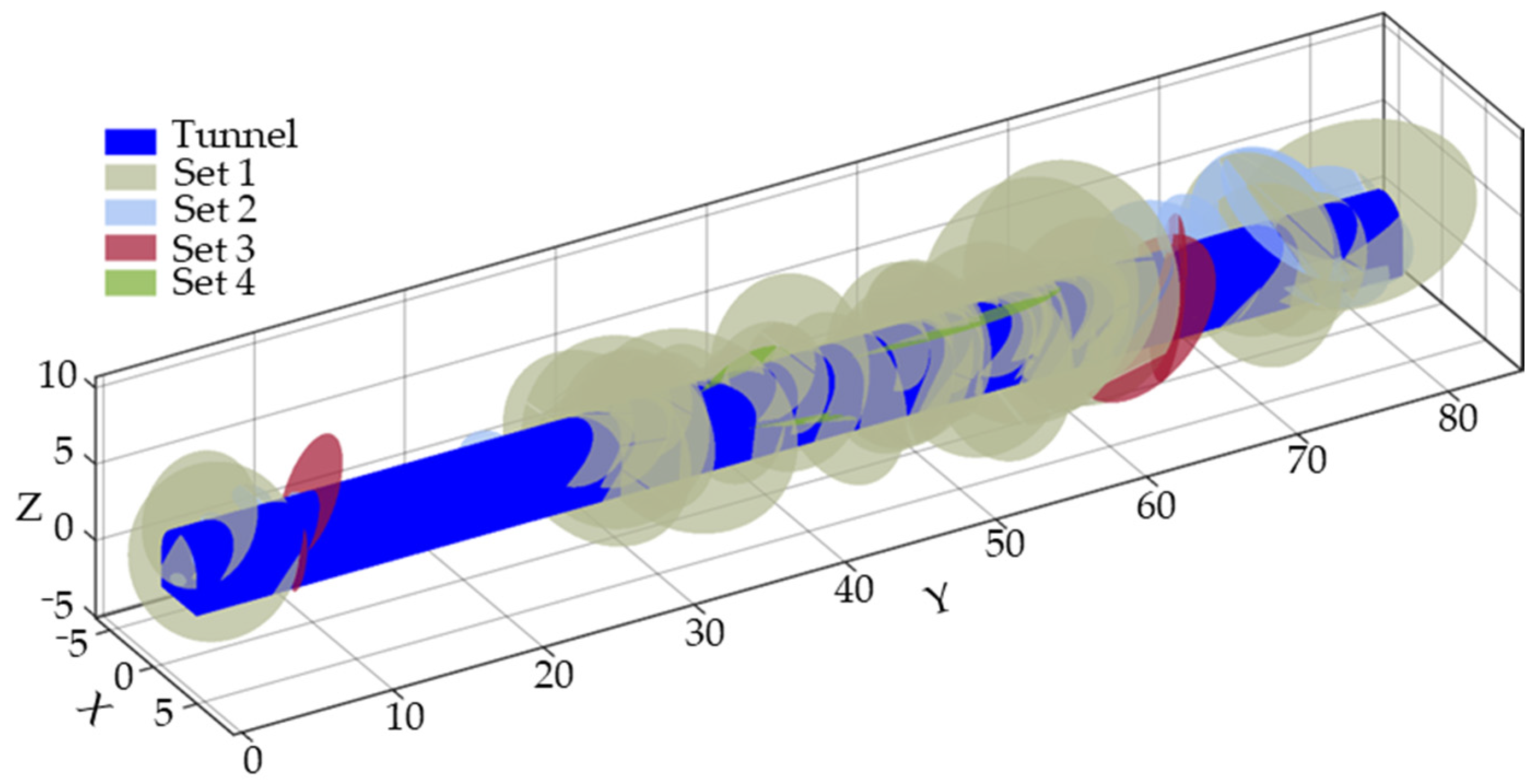
3.6. Fracture Network Modelling
4. Discussion
5. Conclusions
Author Contributions
Funding
Data Availability Statement
Conflicts of Interest
References
- Bonacci, O.; Roje, B.T. Impact of grout curtains on karst groundwater behaviour: An example from the Dinaric karst. Hydrol. Process. 2012, 26, 2765–2772. [Google Scholar] [CrossRef]
- Zou, L.; Håkansson, U.; Cvetkovic, V. Cement grout propagation in two-dimensional fracture networks: Impact of structure and hydraulic variability. Int. J. Rock Mech. Min. Sci. 2019, 115, 1–10. [Google Scholar] [CrossRef]
- Lei, Q.; Latham, J.P.; Tsang, C.F.J. The use of discrete fracture networks for modelling coupled geomechanical and hydrological behaviour of fractured rocks. Comput. Geotech. 2017, 85, 151–176. [Google Scholar] [CrossRef]
- Bruna, P.; Straubhaar, J.; Prabhakaran, R.; Bertotti, G.; Bisdom, K.; Mariethoz, G.; Meda, M. A new methodology to train fracture network simulation using multiple-point statistics. Solid Earth 2019, 10, 537–559. [Google Scholar] [CrossRef]
- Gong, W.; Zhao, C.; Juang, C.H.; Zhang, Y.; Tang, H.; Lu, Y. Coupled characterization of stratigraphic and geo-properties uncertainties–a conditional random field approach. Eng. Geol. 2021, 294, 106348. [Google Scholar] [CrossRef]
- Gao, X.; Zhang, Y.; Hu, J.; Huang, Y.; Liu, Q.; Zhou, J. Site-scale bedrock fracture modeling of a spent fuel reprocessing site based on borehole group in Northwest, China. Eng. Geol. 2022, 304, 106682. [Google Scholar] [CrossRef]
- Guo, H.; Feng, X.; Li, S.; Yang, C.; Yao, Z. Evaluation of the integrity of deep rock masses using results of digital borehole televiewers. Rock Mech. Rock Eng. 2017, 50, 1371–1382. [Google Scholar] [CrossRef]
- Baecher, G.B. Statistical analysis of rock mass fracturing. J. Int. Assoc. Math. Geol. 1983, 15, 329–348. [Google Scholar] [CrossRef]
- Baecher, G.B.; Lanney, N.A.; Einstein, H.H. Statistical description of rock properties and sampling. In Proceedings of the 18th U.S. Symposium on Rock Mechanics (USRMS), Golden, CO, USA, 22–24 June 1977. ARMA-77-0400. [Google Scholar]
- Dershowitz, W.S. Rock Joint Systems. Ph.D. Thesis, Massachusetts Institute of Technology, Cambridge, MA, USA, 1984. [Google Scholar]
- Li, M.; Zhang, Y.; Zhou, S.; Yan, F. Refined modeling and identification of complex rock blocks and block-groups based on an enhanced DFN model. Tunn. Undergr. Space Technol. 2017, 62, 23–34. [Google Scholar] [CrossRef]
- Ma, G.W.; Li, M.; Wang, H.; Chen, Y. Equivalent discrete fracture network method for numerical estimation of deformability in complexly fractured rock masses. Eng. Geol. 2020, 277, 105784. [Google Scholar] [CrossRef]
- Guo, J.; Zheng, J.; Lü, Q.; Sun, H. Empirical methods to quickly select an appropriate discrete fracture network (DFN) model representing the natural fracture facets. Bull. Eng. Geol. Environ. 2021, 80, 5797–5811. [Google Scholar] [CrossRef]
- Koike, K.; Kubo, T.; Liu, C.; Masoud, A.; Amano, K.; Kurihara, A.; Matsuoka, T.; Lanyon, B. 3D geostatistical modeling of fracture system in a granitic massif to characterize hydraulic properties and fracture distribution. Tectonophysics 2015, 660, 1–16. [Google Scholar] [CrossRef]
- Ma, G.W.; Li, T.; Wang, Y.; Chen, Y. The equivalent discrete fracture networks based on the correlation index in highly fractured rock masses. Eng. Geol. 2019, 260, 105228. [Google Scholar] [CrossRef]
- Miyoshi, T.; Elmo, D.; Rogers, S. Influence of data analysis when exploiting DFN model representation in the application of rock mass classification systems. J. Rock Mech. Geotech. Eng. 2018, 10, 1046–1062. [Google Scholar] [CrossRef]
- Lei, Q.; Wang, X. Tectonic interpretation of the connectivity of a multiscale fracture system in limestone. Geophys. Res. Lett. 2016, 43, 1551–1558. [Google Scholar] [CrossRef]
- Pollard, D.D.; Aydin, A. Progress in understanding jointing over the past century. Geol. Soc. Am. Bull. 1988, 100, 1181–1204. [Google Scholar] [CrossRef]
- Schultz, R. Growth of geologic fractures into large-strain populations: Review of nomenclature, subcritical crack growth, and some implications for rock engineering. Int. J. Rock Mech. Min. Sci. 2000, 37, 403–411. [Google Scholar] [CrossRef]
- Wang, R.; Elmo, D. Discrete fracture network (DFN) as an effective tool to study the scale effects of rock quality designation measurements. Appl. Sci. 2024, 14, 7101. [Google Scholar] [CrossRef]
- Mardia, K.; Nyirongo, V.; Walder, A.; Xu, C.; Dowd, P.; Fowell, R.; Kent, J. Markov chain Monte Carlo implementation of rock fracture modelling. Math. Geol. 2007, 39, 355–381. [Google Scholar] [CrossRef]
- Zou, X.W.; Zhou, T.; Li, G.; Hu, Y.; Deng, B.; Yang, T. Intelligent inversion analysis of surrounding rock parameters and deformation characteristics of a water diversion surge shaft. Designs 2024, 8, 116. [Google Scholar] [CrossRef]
- Ma, W.B.; Zou, W.H.; Zhang, J.L.; Li, G. Prediction of shear strength in anisotropic structural planes considering size effects. Designs 2025, 9, 17. [Google Scholar] [CrossRef]
- Green, J. A generalized probability model for sequences of wet and dry days. Mon. Weather Rev. 1970, 98, 238–241. [Google Scholar] [CrossRef]
- Gates, P.; Tong, H. On Markov chain modeling to some weather data. J. Appl. Meteorol. Climatol. 1976, 15, 1145–1151. [Google Scholar] [CrossRef]
- Qi, X.; Li, D.; Phoon, K.; Cao, Z.; Tang, X. Simulation of geologic uncertainty using coupled Markov chain. Eng. Geol. 2016, 207, 129–140. [Google Scholar] [CrossRef]
- Elfeki, A.; Dekking, M. A Markov chain model for subsurface characterization: Theory and applications. Math. Geol. 2001, 33, 569–589. [Google Scholar] [CrossRef]
- Fisher, R.A. Dispersion on a sphere. Proc. R. Soc. Lond. Ser. A Math. Phys. Sci. 1953, 217, 295–305. [Google Scholar] [CrossRef]
- Zhang, L.; Einstein, H.H. Estimating the intensity of rock discontinuities. Int. J. Rock Mech. Min. Sci. 2000, 37, 819–837. [Google Scholar] [CrossRef]
- Priest, S.; Hudson, J. Estimation of discontinuity spacing and trace length using scanline surveys. Int. J. Rock Mech. Min. Sci. Geomech. Abstr. 1981, 18, 183–197. [Google Scholar] [CrossRef]
- Kulatilake, P. Application of probability and statistics in joint network modeling in three dimensions. In Probabilistic Methods in Geotechnical Engineering; CRC Press: Boca Raton, FL, USA, 2020. [Google Scholar]
- Deng, X.; Liu, Q.; Deng, Y.; Mahadevan, S. An improved method to construct basic probability assignment based on the confusion matrix for classification problem. Inf. Sci. 2016, 340, 250–261. [Google Scholar] [CrossRef]
- Cui, L.; Zhang, F.; An, M.; Zhuang, L.; Elsworth, D.; Zhong, Z. Frictional stability and permeability evolution of fractures subjected to repeated cycles of heating-and-quenching: Granites from the Gonghe Basin, northwest China. Geomech. Geophys. Geo Energy Geo Resour. 2023, 9, 18. [Google Scholar] [CrossRef]
- Tao, M.; Ma, L.; Wu, F.; Feng, G.; Xue, Y. Experimental study on permeability evolution and nonlinear seepage characteristics of fractured rock in coupled thermo-hydraulic-mechanical environment: A case study of the sedimentary rock in Xishan area. Eng. Geol. 2021, 294, 106339. [Google Scholar]
- Xue, K.; Zhang, Z.; Jiang, Y.; Luo, Y. Estimating the permeability of fractured rocks using topological characteristics of fracture network. Comput. Geotech. 2023, 157, 105337. [Google Scholar] [CrossRef]
- Tong, H. Determination of the order of a Markov chain by Akaike’s information criterion. J. Appl. Probab. 1975, 12, 488–497. [Google Scholar] [CrossRef]


| Distribution | μx | (σx)2 |
|---|---|---|
| Lognormal | ||
| Exponential | ||
| Gamma |
| Set | θ Range, ° | , ° | φ Range, ° | , ° | Quantity | R | p |
|---|---|---|---|---|---|---|---|
| 1 | 285/360 | 137 | 7/90 | 67 | 434 | 403 | 13.8 |
| 2 | 0/105 | 27 | 10/87 | 63 | 214 | 183 | 6.9 |
| 3 | 205/282 | 197 | 17/89 | 67 | 227 | 204 | 9.9 |
| 4 | 110/201 | 302 | 10/89 | 61 | 330 | 298 | 10.2 |
| (a) Results of the first set of likelihood ratio test statistic calculations | |||
| Statistics | Statistics value | Degree of freedom | 5% Level of significance |
| η01 | 88.09 | 25 | 37.65 |
| η02 | 230.58 | 175 | 206.87 |
| η03 | 466.81 | 1075 | 1152.39 |
| η12 | 142.5 | 150 | 179.58 |
| η13 | 378.72 | 1050 | 1126.5 |
| η23 | 236.22 | 900 | 970.9 |
| η33 | 0 | 0 | 0 |
| (b) Results of the second set of likelihood ratio test statistic calculations | |||
| Statistics | Statistics value | Degree of freedom | 5% Level of significance |
| η01 | 85 | 25 | 37.65 |
| η02 | 159.09 | 175 | 206.87 |
| η03 | 264.54 | 1075 | 1152.39 |
| η12 | 74.08 | 150 | 179.58 |
| η13 | 179.54 | 1050 | 1126.5 |
| η23 | 105.45 | 900 | 970.9 |
| η33 | 0 | 0 | 0 |
| (c) Results of the third set of likelihood ratio test statistic calculations | |||
| Statistics | Statistics value | Degree of freedom | 5% Level of significance |
| η01 | 48.86 | 25 | 37.65 |
| η02 | 118.15 | 175 | 206.87 |
| η03 | 240.02 | 1075 | 1152.39 |
| η12 | 69.29 | 150 | 179.58 |
| η13 | 191.16 | 1050 | 1126.5 |
| η23 | 121.87 | 900 | 970.9 |
| η33 | 0 | 0 | 0 |
| (d) Results of the fourth set of likelihood ratio test statistic calculations | |||
| Statistics | Statistics value | Degree of freedom | 5% Level of significance |
| η01 | 58.58 | 25 | 37.65 |
| η02 | 195.33 | 175 | 206.87 |
| η03 | 394.18 | 1075 | 1152.39 |
| η12 | 136.75 | 150 | 179.58 |
| η13 | 335.6 | 1050 | 1126.5 |
| η23 | 198.85 | 900 | 970.9 |
| η33 | 0 | 0 | 0 |
| (a) AIC values of the first set | ||||
| Order | 0 | 1 | 2 | 3 |
| AIC | −1683.19 | −1721.28 | −1563.78 | 0 |
| (b) AIC values of the second set | ||||
| Order | 0 | 1 | 2 | 3 |
| AIC | −1885.46 | −1920.46 | −1694.55 | 0 |
| (c) AIC values of the third set | ||||
| Order | 0 | 1 | 2 | 3 |
| AIC | −1909.98 | −1908.84 | −1678.13 | 0 |
| (d) AIC values of the fourth set | ||||
| Order | 0 | 1 | 2 | 3 |
| AIC | −1755.82 | −1764.4 | −1601.15 | 0 |
| (a) Correction transition number (Set 1, k = 2.1) | ||||||
| State | 0 | 1 | 2 | 3 | 4 | 5 |
| 0 | 357 | 42 | 15 | 10 | 4 | 5 |
| 1 | 40 | 65.1 | 11 | 9 | 1 | 4 |
| 2 | 18 | 11 | 18.9 | 7 | 3 | 3 |
| 3 | 12 | 7 | 9 | 16.8 | 1 | 0 |
| 4 | 2 | 1 | 2 | 3 | 6.3 | 1 |
| 5 | 5 | 3 | 5 | 0 | 0 | 0 |
| (b) Correction transition probability matrix (Set 1, k = 2.1) | ||||||
| State | 0 | 1 | 2 | 3 | 4 | 5 |
| 0 | 0.82 | 0.1 | 0.03 | 0.02 | 0.01 | 0.01 |
| 1 | 0.31 | 0.5 | 0.08 | 0.07 | 0.01 | 0.03 |
| 2 | 0.3 | 0.18 | 0.31 | 0.11 | 0.05 | 0.05 |
| 3 | 0.26 | 0.15 | 0.2 | 0.37 | 0.02 | 0 |
| 4 | 0.13 | 0.07 | 0.13 | 0.2 | 0.41 | 0.07 |
| 5 | 0.38 | 0.23 | 0.38 | 0 | 0 | 0 |
| (c) Correction transition probability matrix (Set 2, k = 2.05) | ||||||
| State | 0 | 1 | 2 | 3 | 4 | 5 |
| 0 | 0.91 | 0.04 | 0.04 | 0 | 0 | 0 |
| 1 | 0.41 | 0.46 | 0.1 | 0.04 | 0 | 0 |
| 2 | 0.31 | 0.27 | 0.3 | 0.05 | 0.05 | 0.02 |
| 3 | 0.33 | 0.22 | 0.44 | 0 | 0 | 0 |
| 4 | 0.25 | 0.5 | 0.25 | 0 | 0 | 0 |
| 5 | 0.5 | 0 | 0.5 | 0 | 0 | 0 |
| (d) Correction transition probability matrix (Set 3, k = 4) | ||||||
| State | 0 | 1 | 2 | 3 | 4 | 5 |
| 0 | 0.93 | 0.04 | 0.02 | 0.01 | 0 | 0 |
| 1 | 0.49 | 0.35 | 0.11 | 0.04 | 0 | 0 |
| 2 | 0.24 | 0.17 | 0.56 | 0.04 | 0 | 0 |
| 3 | 0.42 | 0.11 | 0.26 | 0.21 | 0 | 0 |
| 4 | 0.67 | 0.33 | 0 | 0 | 0 | 0 |
| 5 | 0.33 | 0.67 | 0 | 0 | 0 | 0 |
| (e) Correction transition probability matrix (Set 4, k = 3.95) | ||||||
| State | 0 | 1 | 2 | 3 | 4 | 5 |
| 0 | 0.9 | 0.07 | 0.02 | 0.01 | 0.01 | 0 |
| 1 | 0.31 | 0.54 | 0.08 | 0.04 | 0.01 | 0.02 |
| 2 | 0.31 | 0.22 | 0.31 | 0.08 | 0.06 | 0.02 |
| 3 | 0.26 | 0.08 | 0.11 | 0.52 | 0.03 | 0 |
| 4 | 0.2 | 0.27 | 0.2 | 0.07 | 0.26 | 0 |
| 5 | 0.17 | 0.5 | 0.17 | 0.17 | 0 | 0 |
| Set | Assume Distribution | Recommended Distribution | ||||
|---|---|---|---|---|---|---|
| 1 | Log-normal | 2.031 | 0.206 | 5.263 | 5.765 | Log-normal |
| Exponential | 1.066 | 1.136 | 13.636 | |||
| Gamma | 2.026 | 0.216 | 5.253 | |||
| 2 | Log-normal | 4.033 | 1.727 | 26.939 | 61.761 | Exponential |
| Exponential | 2.23 | 4.973 | 59.675 | |||
| Gamma | 3.987 | 1.889 | 26.688 | |||
| 3 | Log-normal | 2.171 | 0.113 | 5.305 | 6.066 | Gamma |
| Exponential | 1.112 | 1.237 | 14.838 | |||
| Gamma | 2.17 | 0.116 | 5.306 | |||
| 4 | Log-normal | 1.98 | 0.079 | 4.332 | 4.5 | Log-normal |
| Exponential | 1.01 | 1.02 | 12.241 | |||
| Gamma | 1.979 | 0.081 | 4.331 |
| Set | Density | Location | Orientation | Diameter | |||||
|---|---|---|---|---|---|---|---|---|---|
| Dip | Dip Direction | Fisher Constant | Distribution Constant | Range | |||||
| Range | Mean | Range | Mean | ||||||
| 1 | Markov chain | Uniform | 7/90 | 67 | 285/ 360 | 137 | 13.8 | Log-normal | 0.1/15.9 |
| 2.031/0.206 | |||||||||
| 2 | 10/87 | 63 | 0/105 | 27 | 6.9 | Exponential | 0.9/17.1 | ||
| 2.23 | |||||||||
| 3 | 17/89 | 67 | 205/ 282 | 197 | 9.9 | Gamma | 1.3/14.8 | ||
| 2.17/0.116 | |||||||||
| 4 | 10/89 | 61 | 110/ 201 | 302 | 10.2 | Log-normal | 1/16.3 | ||
| 1.98/0.079 | |||||||||
| Fracture Number | X (m) | Y (m) | Z (m) | Dip Direction (°) | Dip (°) | Diameter (m) |
|---|---|---|---|---|---|---|
| 1 | 2.1 | 0.7 | 4.2 | 287 | 57 | 8.1 |
| 2 | 27.4 | 2.6 | 2.7 | 301 | 88 | 12.3 |
| 3 | 26.4 | 2.7 | 4 | 287 | 46 | 6.5 |
| 4 | 28.5 | 2.7 | 4.3 | 287 | 59 | 8 |
| 5 | 28.5 | 2.9 | 3.6 | 314 | 62 | 11.1 |
| 6 | 31.2 | 1.7 | 2.4 | 292 | 86 | 9.9 |
| 7 | 31 | 2 | 4.1 | 298 | 58 | 6 |
Disclaimer/Publisher’s Note: The statements, opinions and data contained in all publications are solely those of the individual author(s) and contributor(s) and not of MDPI and/or the editor(s). MDPI and/or the editor(s) disclaim responsibility for any injury to people or property resulting from any ideas, methods, instructions or products referred to in the content. |
© 2025 by the authors. Licensee MDPI, Basel, Switzerland. This article is an open access article distributed under the terms and conditions of the Creative Commons Attribution (CC BY) license (https://creativecommons.org/licenses/by/4.0/).
Share and Cite
Xia, N.; Nie, W.; Yang, Z.; Wu, Y.; Li, T. Application of Curtain Grouting for Seepage Control in the Dongzhuang Dam: A 3D Fracture Network Modeling Approach. Buildings 2025, 15, 2415. https://doi.org/10.3390/buildings15142415
Xia N, Nie W, Yang Z, Wu Y, Li T. Application of Curtain Grouting for Seepage Control in the Dongzhuang Dam: A 3D Fracture Network Modeling Approach. Buildings. 2025; 15(14):2415. https://doi.org/10.3390/buildings15142415
Chicago/Turabian StyleXia, Ning, Wen Nie, Zhenjia Yang, Yang Wu, and Tuo Li. 2025. "Application of Curtain Grouting for Seepage Control in the Dongzhuang Dam: A 3D Fracture Network Modeling Approach" Buildings 15, no. 14: 2415. https://doi.org/10.3390/buildings15142415
APA StyleXia, N., Nie, W., Yang, Z., Wu, Y., & Li, T. (2025). Application of Curtain Grouting for Seepage Control in the Dongzhuang Dam: A 3D Fracture Network Modeling Approach. Buildings, 15(14), 2415. https://doi.org/10.3390/buildings15142415