FS-DDPG: Optimal Control of a Fan Coil Unit System Based on Safe Reinforcement Learning

Abstract

To optimize the control of fan coil unit (FCU) systems under model-free conditions, researchers have integrated reinforcement learning (RL) into the control processes of system pumps and fans. However, traditional RL methods can lead to significant fluctuations in the flow of pumps and fans, posing a safety risk. To address this issue, we propose a novel FCU control method, Fluctuation Suppression–Deep Deterministic Policy Gradient (FS-DDPG). The key innovation lies in applying a constrained Markov decision process to model the FCU control problem, where a penalty term for process constraints is incorporated into the reward function, and constraint tightening is introduced to limit the action space. In addition, to validate the performance of the proposed method, we established a variable operating conditions FCU simulation platform based on the parameters of the actual FCU system and ten years of historical weather data. The platform’s correctness and effectiveness were verified from three aspects: heat transfer, the air side and the water side, under different dry and wet operating conditions. The experimental results show that compared with DDPG, FS-DDPG avoids 98.20% of the pump flow and 95.82% of the fan flow fluctuations, ensuring the safety of the equipment. Compared with DDPG and RBC, FS-DDPG achieves 11.9% and 51.76% energy saving rates, respectively, and also shows better performance in terms of operational performance and satisfaction. In the future, we will further improve the scalability and apply the method to more complex FCU systems in variable environments.

1. Introduction

In the global context, the building sector accounts for over 35% of the world’s energy consumption and nearly 40% of energy-related carbon dioxide emissions [1]. According to projections by the International Energy Agency (IEA) [2], the peak power load in countries with low HVAC penetration is expected to rise by approximately 45% by 2050. This tremendous growth has drawn attention to the management of HVAC systems and energy efficiency. Therefore, it is crucial to improve the efficiency of HVAC systems to reduce energy consumption in the building sector.

Previous studies has mainly focused on air-conditioning heating and cooling sources, with little attention given to terminal air-conditioning equipment, especially fan coil units. The FCU air-conditioning system is the most widely used HVAC subsystem in public facilities [3]. Since FCU has many widely used scenarios, long-term operation and high energy consumption, it is of great significance to study more energy-saving control methods [4]. However, the control parameters of FCU systems involve both linear and nonlinear relationships, and the cooling load constantly fluctuates with the building environment, giving rise to different operating conditions of the FCU. Therefore, optimizing the control of FCU systems remains an urgent problem to be solved.

At present, common control methods for FCUs merely focus on indoor temperature as the control target, including model-based control (MBC) methods [5]; model-free control (MFC) methods [6]; rule-based control (RBC); proportional, integral, derivative (PID) control; and so on. Although naive models are better fit for committed optimization, their inferior precision will impact the control performance. To address these issues, researchers tend to adopt MFC methods [7]. Among MFC methods, RBC methods that rely on expertise are the most commonly used, such as using PID in FCU control to track set points [8]. In addition, because the control parameters are fixed, these methods are not well suited to specific FCU systems [9]. These control methods, due to their ease of deployment, are widely used in practical projects. However, the existing rule-based FCU control methods are relatively stable with few changes, leading to higher energy consumption.

Currently, with the continuous development of artificial intelligence and machine learning (ML), these methods will be further studied and applied in the FCU field [10]. Compared to MBC methods, ML performs better in dynamic environments while learning from real-time data. Compared with MFC methods, ML is capable of accommodating dynamic conditions for capturing complicated system relationships [11]. RL is a method of using ML without relying on physical models. The principle of this method is that the agent will seek the optimal strategy through interaction with the environment. The agent takes action and adjusts its strategy based on rewards from environmental feedback to continuously improve its performance [12]. RL is especially fit for complex environments that need long-range planning. Researchers have already tried to apply RL in the FCU field. RL, with its ability to search for optimal strategies in large-scale state spaces, enables FCU systems to find the most optimal control strategies [13].

However, when traditional RL methods are used to control FCU systems, in some complex and demanding real-world scenarios, collecting data through a trial-and-error method is not only costly but also leads to drastic changes in air and water flow rates within a short period, posing safety risks, as illustrated in Figure 1. The figure depicts part of the fluctuations in water and air flow rates, with the abscissa representing the training episodes and the ordinate showing water and air flow rates. The blue curve represents the changes in water flow, with red points indicating control points where there are abrupt changes in water flow. It is evident that traditional RL control of water pump flow often results in volatile control points (e.g., from 80 to 700 kg/h, and from 700 to 80 kg/h). The orange curve represents the changes in air flow, with red points marking control points where there are abrupt changes in air flow. Similarly, traditional RL control of the air fan flow frequently leads to volatile control points (e.g., from 100 to 1200 m³/h, and from 1200 to 100 m³/h). When the air flow rate of the fan fluctuates sharply, it will lead to unstable air flow and reduce comfort. In addition, it will lead to excessive wear of motors, bearings, etc., and shorten the life of the equipment. When the water flow of the pump fluctuates dramatically, it may cause pressure fluctuations in the pipeline, resulting in pipeline damage. In addition, it will cause overload of the pump body and shorten its service life. Therefore, RL methods need to take safety factors and stability into account and integrate them with traditional control strategies to ensure the long-term and stable operation of FCU systems.

To address the aforementioned challenges, this paper proposes an improved FCU control strategy based on safe reinforcement learning (SRL) and the FS-DDPG control method. The sequential decision problem is modeled as a constrained Markov decision process. This method limits the perceived action space of the agent during the decision-making process by adjusting the constraint tightening in real time, focusing not only on maximizing long-term rewards, but also on how to follow specific security constraints during the decision-making process. This method aims to optimize the regulation of water and air flow within the FCU system, mitigating the impact of action fluctuations on equipment, reducing operational stress, lowering energy consumption and ultimately improving occupant comfort.

The main contributions are as follows:

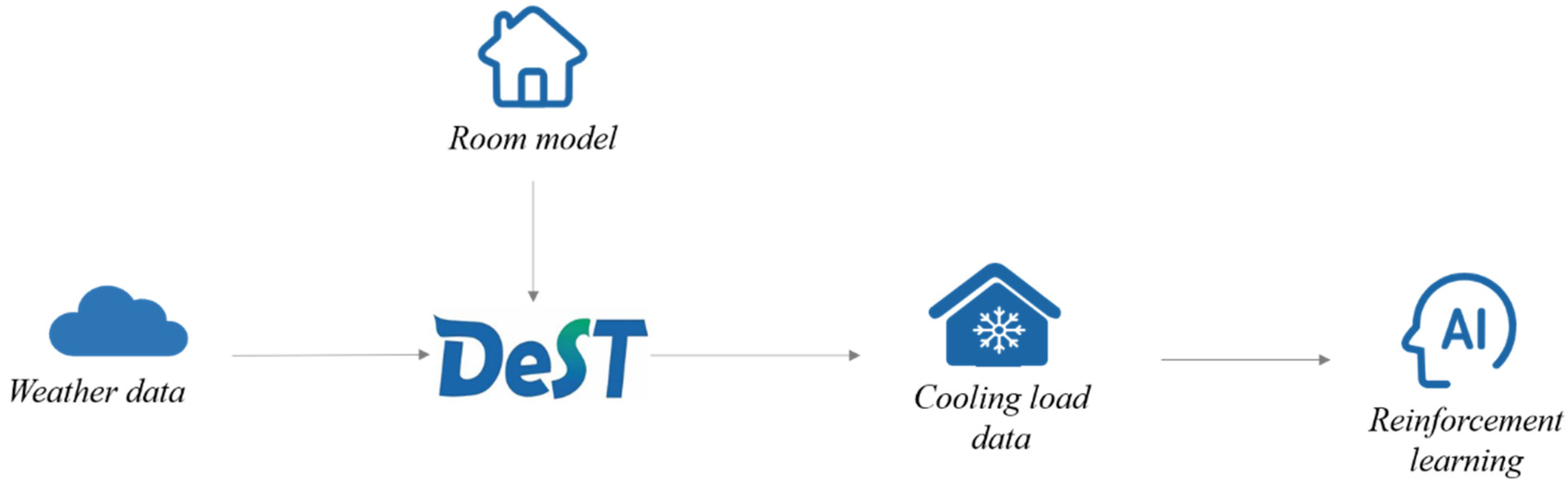
• Based on historical weather data, an office room model was established by using the DeST to calculate the required cooling load for the corresponding period. A heat and mass transfer model for an FCU (incorporating both the theory of thermal and moisture exchange as well as the calculation of parameters within the model) was constructed using Python, which was also validated for its feasibility.
• To address the issue of significant system fluctuations caused by the use of RL methods in controlling the FCU process, the FCU control process is modeled as a constrained Markov decision process. A penalty term regarding process constraints is added to the actual reward function, and constraint tightening is introduced to limit the action space perceived by the agent.
• We propose the FS-DDPG algorithm to optimize the control strategy of an FCU based on reinforcement learning. Compared with the traditional RL algorithm, FS-DDPG not only seeks the maximum reward but also restrains the violent action fluctuation in the control process and greatly reduces the risk of equipment damage caused by the large-scale regulation of the unit.
• The experimental results indicate that this method demonstrates high generalizability and stability, exhibiting significant adaptability in dynamic environments. It not only meets the cooling load requirements within a room while reducing system energy consumption but also ensures the long-term stable operation of the system to the greatest extent. The code and FCU model have been published for future research on the referenced website (available online: https://github.com/leecy123123/fcu_1.git (accessed on 10 January 2025)).

In Section 1, the control method and research status of fan coils are introduced, and then the significance of fan coil control based on SRL is introduced. In Section 2, different control strategies and the application of RL in optimizing system stability and energy efficiency are introduced. In Section 3, the dynamic simulation model of a fan coil system is established based on the actual fan coil system. In Section 4, Markov modeling and control flow based on the FS-DDPG algorithm are introduced. In Section 5, compared with the experimental results of other control methods, the effectiveness of the proposed method in terms of safety and energy saving is analyzed from various angles. In Section 6, the research content is summarized and the future development of the control method is prospected.

2. Related Work

FCU systems have been extensively applied in numerous construction sectors recently. Its performance optimization can be achieved through two control strategies: model-based control and model-free control. Model-based control strategies rely on pre-constructed physical models, whereas model-free control strategy directly manipulates FCU systems through real-time feedback, without depending on pre-built models [14,15,16].

In the early stages, simple rule-based control (RBC) methods were used to manage FCU systems, leading these systems to maintain specific states, which often resulted in indoor temperatures being too high or too low. Through extensive practical application, the PID (proportional, integral, derivative) control algorithm has been gained widespread recognition in the control field for its excellent stability and robustness. As classical control theory has advanced, various complex control strategies based on the traditional PID method have emerged. Li et al. [17] proposed to use a fractional-order PID controller of indoor temperature and a three-position controller of air supply volume to work together to achieve the desired indoor temperature. Li et al. [18] configured this fractional-order PID control system by adjusting the satisfactory values of five parameters of the fractional-order PID controller for indoor temperature. The results show that the related control performance indices of the proposed control system meet the design requirements of comfortable air-conditioning. Despite the widespread application of PID control methods in air-conditioning, since the break frequency of PID was challenging to align with the system model’s break frequency, their effectiveness was limited in complex and nonlinear systems, resulting in a suboptimal control performance.

In recent years, model-based control (MBC) has garnered significant attention in the application of FCU systems. MBC as a form of supervisory control offers good stability and multi-objective rolling optimization. However, the effectiveness of MBC relies heavily on accurate pre-built models and requires precise data on both indoor and outdoor architectural parameter changes [19]. If there is a substantial discrepancy between the mathematical model and the actual FCU system, the control effectiveness of MBC is difficult to guarantee. In model-based control, model predictive control (MPC) is the most commonly used method. Zhao et al. [20] developed a distributed MPC architecture for fan-coil systems, using a hybrid Beetle-antenna search–Particle Swarm Optimization (BAS-PSO) algorithm to optimize the local MPC online. The experimental results show that compared with the traditional PID control, the distributed MPC realizes coordinated multi-zone indoor temperature regulation, and the energy saving rate is 16.23%. Sanama [21] proposed a PID predictive model controller, which can effectively improve indoor air quality and achieve a satisfactory control effect. Martin Chevitch [22] developed an energy model oriented towards control, combining model and identification methods to identify FCU systems, thus achieving predictive building control.

Model-free control (MFC) methods are independent of the FCU model, boasting high adaptability and real-time response capabilities, enabling quick adaptation to environmental changes and uncertainties in the system. However, MFC methods rely heavily on data quality and require higher computational resources. Compared to MBC methods, MFC might fall short in certain performance indicators, such as system energy consumption and operational performance, but it remains within an acceptable range and may be more suitable in certain application scenarios. In the realm of model-free control methods, Guillen et al. [23] built the RELAP5-3D/LSTM model to analyze FCU faults. LSTM is used to predict the FCU inlet temperature according to PMIS. RELAP5-3D simulates the measured FCU inlet temperature and the temperature predicted by LSTM to obtain the FCU outlet temperature. The abnormal operation of an FCU can be detected by comparing the actual value of the FCU outlet temperature with the predictive value. Lin and others [24] developed an optimization control strategy for Heating, Ventilation and Air-Conditioning (HVAC) systems, including temperature control for fan coil units (FCUs). Their proposed strategy includes dynamically setting the FCU temperature according to changes in outdoor temperature; collecting the set FCU temperatures and converting them into the cooling capacity required by the chilled water system; and using genetic algorithms to calculate the minimum energy consumption of the HVAC system. However, machine learning relies heavily on data. If there are insufficient data, poor quality data or overfitting, system performance might be impacted severely [25].

Currently, RL is regarded as a valid method in model-free learning. Its applications in fields such as HVAC have already shown significant success, highlighting its enormous potential in control optimization and energy efficiency. However, the application of RL in the FCU field remains relatively limited. Applying RL algorithms to control FCU systems offers the promise of improving user comfort, optimizing indoor air quality and reducing energy consumption. Chen et al. [26] proposed adopting the DQN algorithm to adjust the air supply volume of an FCU in an office building. The proposed method can improve the satisfaction rate of joint control of indoor temperature and relative humidity. Zhang et al. [13] introduced a DDPG-PK algorithm to regulate the air and water flow of an FCU, aiming to achieve minimal energy consumption while satisfying the cooling load requirements. Unlike MFC methods, this algorithm integrates expert knowledge into the DRL, reducing initial exploration and improving initial performance. However, when controlling FCU systems with traditional RL algorithms, agents may take high-risk exploration actions with significant fluctuations, which are unacceptable for practical FCU systems. Therefore, the concept of SRL is considered in the optimization of FCU system control. Unlike existing studies using Deep Reinforcement Learning (DRL) methods, SRL methods prioritize safety in the learning and decision-making process. This ensures that while pursuing optimal performance, the system places greater emphasis on avoiding dangerous actions and minimizing potential damage to the system. By reducing risks and enhancing system robustness, SRL helps to establish a long-term sustainable FCU system. Hence, researching the use of SRL in FCU control is of significant importance. To address these issues, this paper proposes an FS-DDPG method to regulate the air and water flow rates of the FCU system. This method ensures the system’s stability and safety while meeting the required cooling load with minimal energy consumption. Compared with conventional RL control methods, this method innovatively incorporates policy constraints into the modeling process, thereby constraining actions in FCU systems and ensuring its long-term automated operation.

Additionally, FS-DDPG exhibits strong adaptability and can be applied to various types of HVAC systems and similar control systems. However, its generalizability is influenced by factors such as environmental stability, data quality and system complexity. Therefore, in broader application scenarios, it may be necessary to adjust the assumptions and optimization strategies of the method according to the specific control system.

3. Case Study

This paper tries to optimize an FCU system to satisfy cooling demands while controlling energy consumption and ensuring the safety of the unit’s equipment. The effect of this method is measured with computer simulations. The FCU system operates from Monday to Friday, 7:00 a.m. to 9:00 p.m., depending on the required scenario.

Given the complexity of designing and simulating FCUs, developing a model with high computational accuracy, fast processing speed and ease of data analysis is of significant value and importance for long-term research on FCUs.

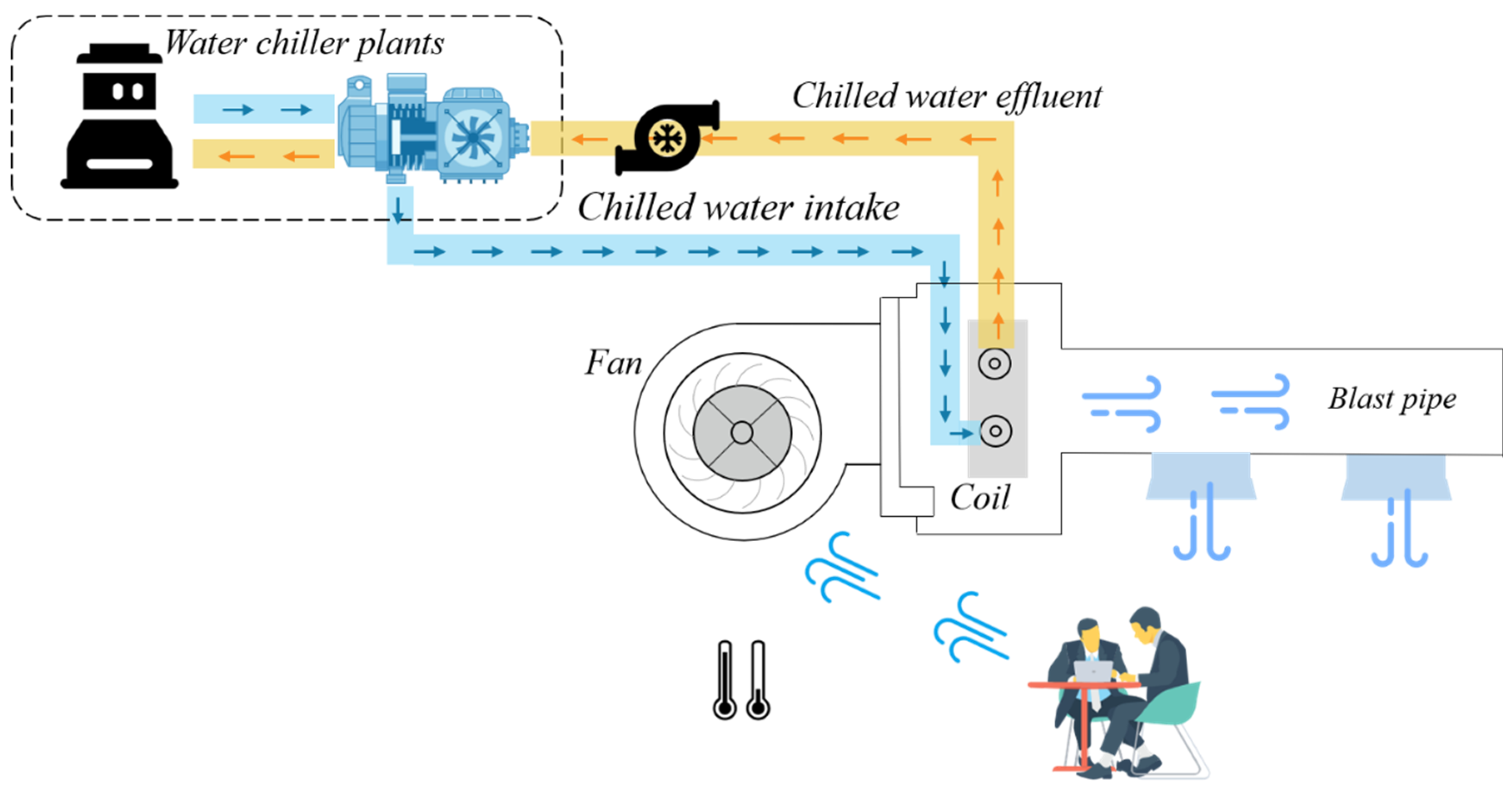
3.1. System Operation Overview

The FCU system is a terminal device of air-conditioning systems, consisting of a fan, controller and coils (air heat exchangers). Chilled water provided by refrigeration equipment (such as chillers) enters the terminal coils under the pressure generated by the chilled water pump. To precisely control the water flow rate in each area, shut-off valves are installed at the front end of the fan coils. As the chilled water flows through the terminal fan coil, the temperature of the copper water pipes inside the coil is lowered through forced heat transfer within the pipes. In return, it reduces the temperature of the aluminum fins mounted on the water pipes. When the fan operates, it blows the air between the aluminum fins into the room, enabling the FCU system to satisfy the indoor cooling load. The chilled water then returns to the chiller plants to complete the cycle. The temperature difference of the chilled water before and after the heat exchange process represents the cooling capacity of the FCU system. The overall working schematic is as depicted in Figure 2.

In the control issues of the FCU, there is a correlation between different cooling loads and the control of water and air flow rates in the FCU system. Therefore, in this paper, the cooling load is used as the basis for controlling the FCU system. The water and air flow rates of the FCU system are treated as the control actions of the controller.

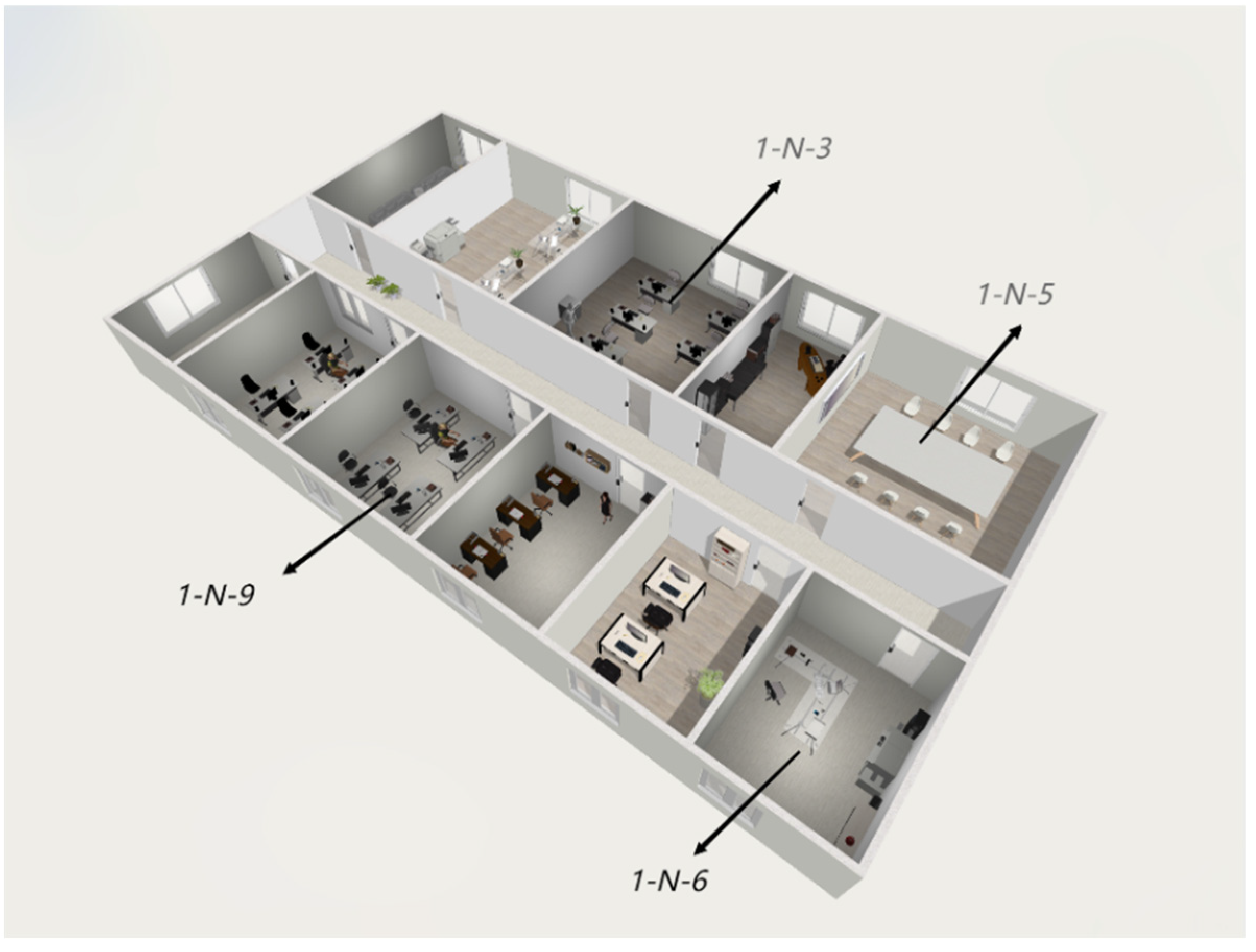
3.2. Building Room Model and Simulating Cooling Load

This paper utilizes the DeST software (Version number: 20230713) for simulating the cooling load of rooms. DeST is a software platform designed for the simulation of building environments and HVAC systems, aimed at assisting architects and engineers in evaluating the energy performance of building designs during the early stages of the design process. A room model of an office building was established using DeST. Ten years of weather data were input to calculate the room’s cooling load, which is used for the subsequent optimization control of the FCU system by the RL algorithm. The cooling load here is only used as the state setting in the RL algorithm and is not involved in the training process, which will be detailed in later chapters. The control process is shown in Figure 3.

In this paper, a single-story room model is established in DeST, configured as a floating structure. Eleven rooms and one corridor are set up, with each room equipped with windows. The top-down view of this room is illustrated in Figure 4.

In the room model, 11 rooms and one corridor are established (numbered 1-N-1, 1-N-2, …, 1-N-12).

Table 1. Basic room attributes configuration.

Room Number	Room Function	Room Area	Interior Design Temperature
1-N-1	Lounge	32	26
1-N-2	Office	96	25
1-N-3	Office	96	25
1-N-4	Office	32	25
1-N-5	Conference Room	96	26
1-N-6	Office	64	25
1-N-7	Office	64	25
1-N-8	Office	64	25
1-N-9	Office	64	25
1-N-10	Office	64	25
1-N-11	Supply Room	32	No Set
1-N-12	Hallway	176	No Set

shows the usage, area and set room temperature for each room. Notably, rooms 1-N-11 and 1-N-12, being a storeroom and a corridor, respectively, are not equipped with FCUs but are included in the heat exchange calculations with other rooms in the DeST software. The maximum thermal disturbance power of the fixed equipment is set according to the rated power of the fixed equipment of 12 W. The occupancy schedule follows the basic settings for corresponding room usage in DeST, without additional thermal disturbances or ventilation. The equipment schedule aligns with the room’s usage.

After establishing a basic room model in DeST, the weather data from 2012 to 2022 (including 2 m air temperature, surface pressure, surface temperature, dew point temperature, relative humidity, east wind speed, north wind speed, total solar irradiance, net solar irradiance, amount of precipitation, evaporation capacity and ultraviolet intensity) were downloaded from the US National Ocean Service [27], with data from 2012 to 2021 used for the training set and data from 2022 used for testing. The metrics included in this data set are shown in

Table 2. Statistical analysis of weather data from 2012 to 2022.

Metrics	Maximum Value	Minimum Value	Median	Mean Value	Unit
2 m air temperature	37.26	−7.61	18.59	17.82	°C
Surface pressure	1041.42	981.76	1016.41	1015.94	$\mathrm{h}\mathrm{P}\mathrm{a}$
Surface temperature	38.38	−8.08	17.98	17.17	°C
Dew point temperature	28.93	20.55	13.66	13.34	°C
Relative humidity	99.99	15.09	80.72	76.93	%
East wind speed	8.84	10.95	−0.41	0.32	$\mathrm{m}/\mathrm{s}$
North wind speed	8.38	−13.50	−1.03	0.75	$\mathrm{m}/\mathrm{s}$
Total solar irradiance	3653.08	0	20.46	583.70	$\mathrm{J}/{\mathrm{m}}^2$
Net solar irradiance	3096.26	0	17.71	499.52	$\mathrm{J}/{\mathrm{m}}^2$
Amount of precipitation	14.24	0	0	0.18	$\mathrm{m}\mathrm{m}$
Evaporation capacity	0.04	0.76	-0.04	0.11	$\mathrm{m}\mathrm{m}$
Ultraviolet intensity	410.87	0	2.74	65.62	$\mathrm{J}/{\mathrm{m}}^2$

.

The raw weather data from ClimateData.accdb were pre-processed using Microsoft Access to match the format required in the DeST simulation. The cooling load for the cooling season from 1 May to 30 September was then calculated by DeST based on the weather data. Additionally, ineffective cooling load data were eliminated, focusing only on human activity hours, specifically from 7:00 a.m. to 9:00 p.m., amounting to 14 h per day. This process yielded cooling load values for ten rooms over eleven years, excluding rooms 1-N-11 and 1-N-12. After processing, each room’s cooling load data comprised 23,562 entries with a resolution of 1 h. Figure 5 shows the thermal maps of 2142 cooling load data for room 1-N-6 in 2021.

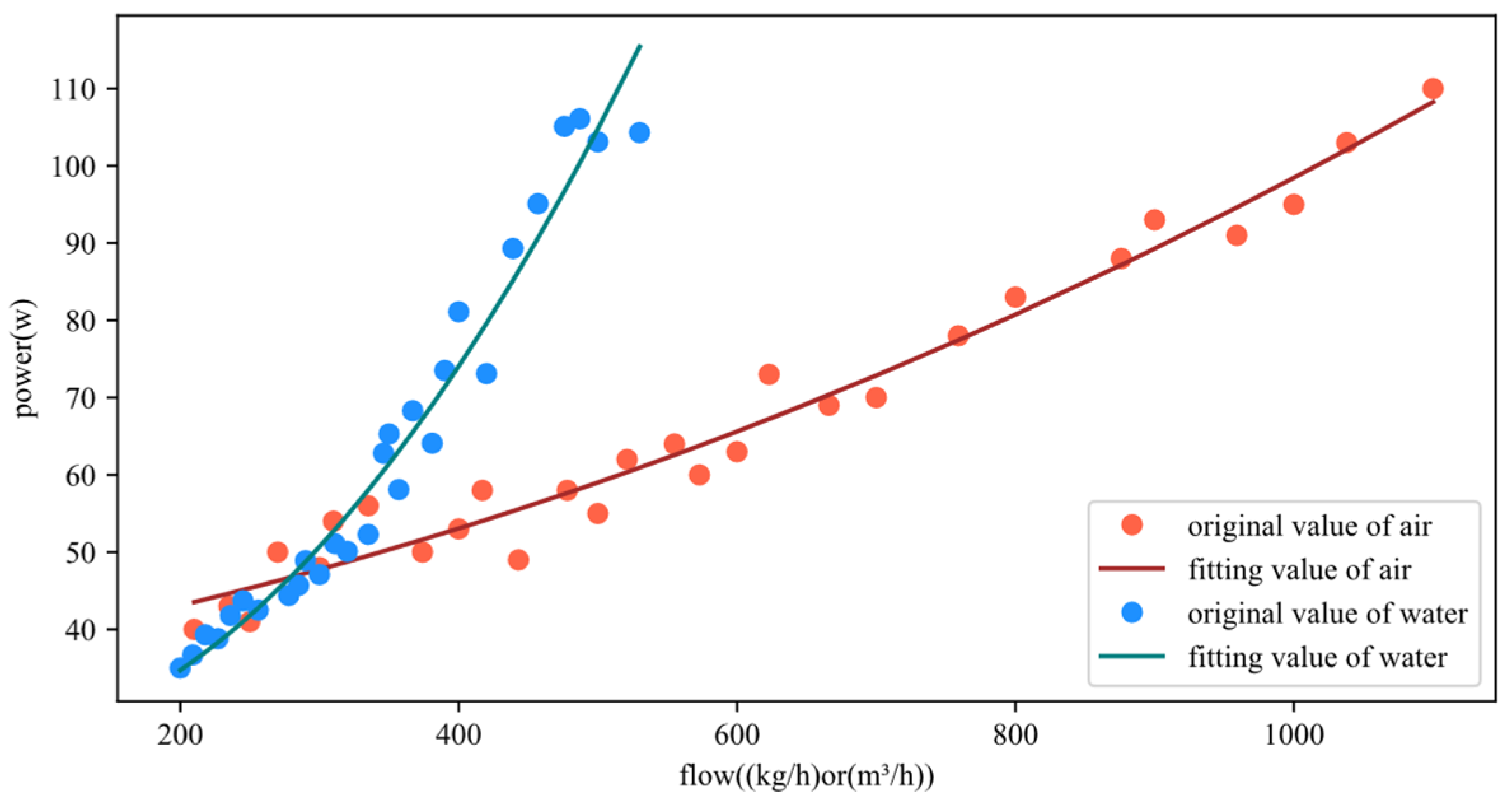
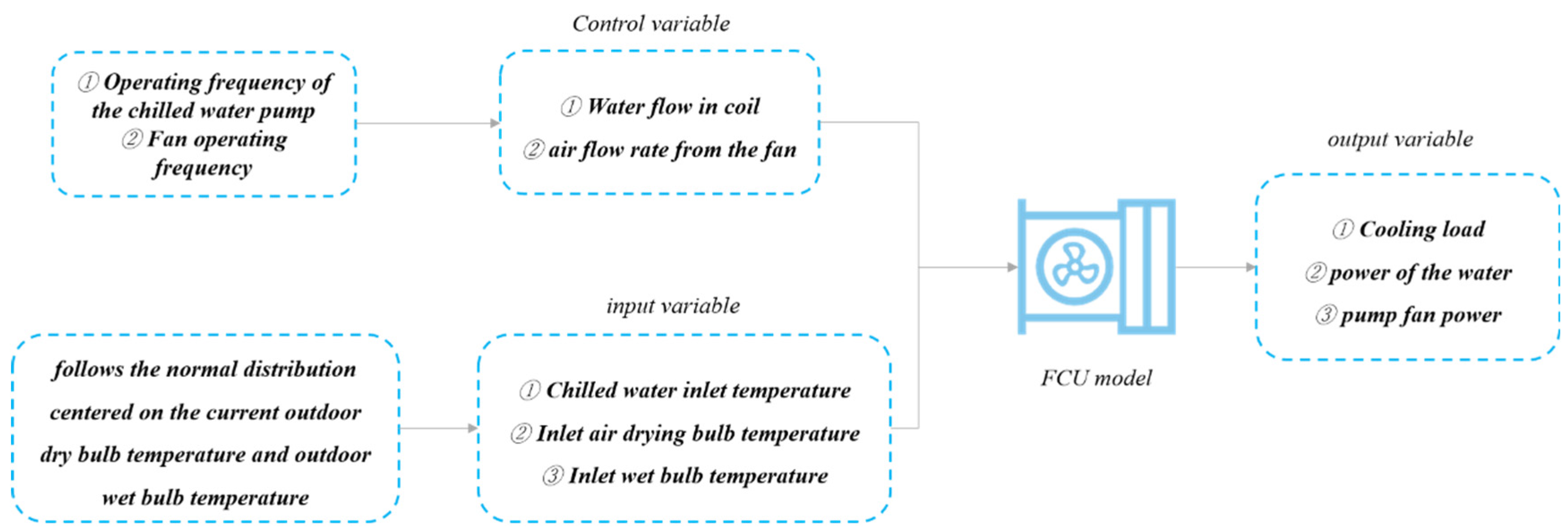
3.3. Modeling of Fan Coil

To validate the working principle of the control system algorithm, this section establishes an input–output simulation model for the FCU, as illustrated in Figure 6.

The control variables of the system are set as the water flow inside the coil and the air flow discharged by the fan, which are adjusted through the control of the pump and the fan, respectively. This allows for more precise and rapid adjustment of indoor temperature and humidity, while also more accurately matching system demands to optimize energy efficiency. These variables serve as the control points for the subsequent control algorithm analysis. The input variables are the inlet temperature of the chilled water, the dry bulb temperature of the incoming air and the relative humidity of the incoming air. To simplify the model, the outlet temperature of the chilled water is fixed at 7 degrees Celsius, and the dry bulb temperature and relative humidity of the incoming air are set to follow a normal distribution centered around the current outdoor dry bulb and wet bulb temperatures. The model’s output measures the actual cooling capacity of the FCU, along with the corresponding water flow and air flow, and the power consumption of both the pump and the fan.

The physical parameters of the FCU system used in this paper are shown in Appendix A. The model assumptions and detailed calculations of the FCU are shown in Appendix B. Appendix B implements the calculation process of the FCU system, but its validity needs to be verified by experiments. The actual experimental data of a particular model of the FCU system are compared with the calculated results of the model, and the results are shown in Appendix C.

4. Methodology and Control Process

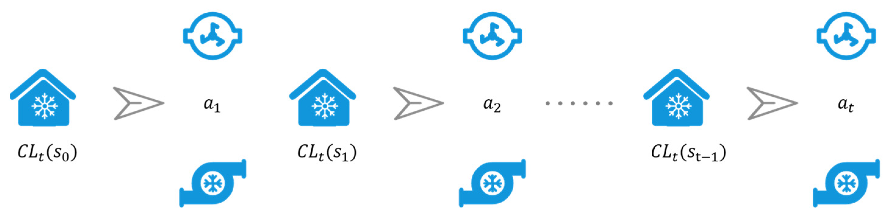
To ensure the safe operation of the FCU system and to prevent significant fluctuations in the actions of the chilled water pump and the fan, a novel energy-saving control method is proposed. This method, named as the FS-DDPG method, specifically addresses the issue of potential severe action fluctuations that may arise in the DDPG control method. By optimizing the actions provided by the actor network in DDPG, FS-DDPG can stabilize the air flow and water flow rates of the fan and pump. Consequently, FS-DDPG not only reduces energy consumption and but also protects the equipment.

4.1. CMDP Modeling

When DRL is used to solve control problems, it is necessary to model the controlled problem as a Markov decision process. However, the uncertainty and uncontrollable factors in the environment are ignored in the traditional MDP, which leads to the instability and performance degradation of the model. To solve these problems, the control process needs to be modeled as a constrained Markov decision process (CMDP). In CMDP, the agent needs to find a strategy that satisfies the constraints so that the agent chooses the optimal action in each state to obtain the maximum return, while satisfying additional constraints. In this section, the control process of the FCU system is modeled as a CMDP, which mainly involves the setting of state, action, cost and reward, as follows:

• State

When considering the modeling of Markov decision processes, the properties of the controlled environment are often defined as states in SRL. In this paper, the cooling load considering the current demand is the basis of controlling the water flow and air flow of the FCU system. Hence, the cooling load required at the current moment is taken as the state in SRL, as shown in Equation (1):

$$\begin{array}{c}\begin{array}{c}s=\left\{C{L}_t\right\}\end{array}\end{array}$$

(1)

2.

Action

In the FCU control process, the control node of the system is usually defined as the air flow of the fan and the water flow of the pump. Thus, water flow and air flow are set as actions in SRL, as shown in Equation (2):

$$\begin{array}{c}\begin{array}{c}a=\left\{flo{w}_{water},flo{w}_{air}\right\}\end{array}\end{array}$$

(2)

3.

Reward

In the control process, not only does the cooling output of the FCU system need to satisfy the cooling load demand of the room, but it is also necessary to ensure the relative stability of the air flow and water flow. Therefore, when the cooling output generated by the system satisfy the needed cooling load of the room and the flow rate of the fan and the pump changes smoothly, the environment will reward the behavior under the current state. Moreover, the reward is negatively correlated with $Q_{FCU}-C{L}_t$, $diff$ and $P_{water}+P_{air}$.

$$\begin{array}{c}\begin{array}{c}r=-k_1\left(1-e^{-{\displaystyle \frac{{\left(Q_{FCU}-C{L}_t\right)}^2}{2\times {\left(0.1\times C{L}_t\right)}^2}}}\right)-\left(P_{water}+P_{air}\right)\end{array}-\lambda ·diff\end{array}$$

(3)

where $Q_{FCU}$ is the actual generated cooling capacity, $P_{water}$ is the water flow related power, $P_{air}$ is the wind flow related power, $k_1$ are hyperparameters for meeting the current cooling load, $\lambda$ is the penalty term weight and $diff$ is an indicator of action continuity.

During optimization, there is a trade-off between energy consumption, safety performance and operational performance. For instance, reducing energy consumption might slow down the system response and lead to decreased satisfaction. Therefore, two weight factors, $k_1$ and $\lambda$, are used in the reward function to balance energy efficiency, operational performance and safety performance. After ensuring that the values of each part are in the same proportion, the sensitivity analysis experiment is performed to set $k_1$ to 330 and $\lambda$ to 10. These coefficients ensure that while maintaining satisfaction and safety performance, the system can still minimize energy consumption and avoid performance degradation caused by excessive energy optimization.

As shown in Figure 7, based on the aforementioned mode, the agent firstly obtains the required cooling load, then selects water flow and air flow as actions. After acting on the FCU, the agent obtains a reward and the state moves to the next required cooling load.

4.

Constraint

In the CMDP framework, $C$ is considered as a security measure of system actions to balance cumulative rewards with the security of the system. We consider the reward function as the relationship between $C$ and $R$, and adjust the objective function of CMDP, as shown in Equation (4):

$$\begin{array}{c}{J}_{CMDP\left(\pi \right)}=J\left(\pi \right)-\lambda \cdot \mathbb{E}\left[{\displaystyle \sum _{t=0}^{\mathrm{\infty }}} {\gamma }^{t}C\left(a_t\right)\mid s_0\sim {\rho }_0,a_t\sim \pi \left(\cdot \mid s_t\right)\right]\end{array}$$

(4)

$\lambda$ is a hyperparameter used to balance reward and safety constraints. In this problem, $C\left(a\right)$ is regarded as the relative error of the output action and is defined in Equation (5). $C\left(a\right)$ consists of $C_1\left(a\right)$ and $C_2\left(a\right)$, which are defined in Equation (6):

$$\begin{array}{c}C\left(a\right)={w_1\ast C}_1\left(a\right)+{w_2\ast C}_2\left(a\right)\end{array}$$

(5)

$$\begin{array}{c}\begin{array}{c}{C}_1\left(a\right)={\displaystyle \frac{\left|a_{water}-a_{water\_pre}\right|}{a_{water}}}\\ C_2\left(a\right)={\displaystyle \frac{\left|a_{air}-a_{air\text{\_}pre}\right|}{a_{air}}}\end{array}\end{array}$$

(6)

where $w_1$ and $w_2$ are weight parameters, $a_{water}$ is the water flow at time $t$, $a_{water\text{\_}pre}$ is the water flow at time $t-1$, $a_{air}$ is the air flow at time $t$ and $a_{air\text{\_}pre}$ is the air flow at time $t-1$.

4.2. Action Constraint

In DRL tasks, by adding the constraint on the action to the reward function, the behavior of the agent can be restricted to ensure the security of the FCU system. This section presents how to integrate action constraints into the RL framework to achieve SRL control. This method aims at reducing the uncertainty generated by algorithms in unknown environments, thereby enhancing the stability of the learning process.

4.2.1. Punishment Constraint Method

In continuous-action spaces, constraints can be implemented by introducing a penalty term into the reward function. Assuming the original reward function is defined as $reward=r\left(s,a,s^{\prime }\right)$, where $s$ is the current state, $a$is the action selected by the agent and $s^{\prime }$ is the next state. To ensure the safety of actions, we reformulate the reward function as Equation (7):

$$\begin{array}{c}\widehat{r}\left(s,a,s^{\prime }\right)=r\left(s,a,s^{\prime }\right)-\lambda \cdot C\left(a\right)\end{array}$$

(7)

where $\widehat{r}$ is the rewritten reward function, $\lambda$ is the regularization parameter, which regulates the strength of the punishment and $C\left(a\right)$ is calculated by $C_1\left(a\right)$ and $C_2\left(a\right)$ in Equation (5).

Based on multiple repeated independent experiments and experience, the weight coefficients $w_1$ and $w_2$ are set to 0.4 and 0.6, and $\lambda$ is set to 10. In order to control the relative error to be as small as possible and keep the output action of the agent (water flow and air flow of the FCU system) continuous and stable, $\lambda \cdot C\left(a\right)$ is expressed as $r_c$, which incorporates the relative error into the reward mechanism of RL. Therefore, a piecewise function is designed so that the smaller the relative error, the greater the reward value, as shown in Equation (8):

$$\begin{array}{c}{r}_c=\left\{\begin{array}{c}1-C\left(a\right),ifC\left(a\right)\le \beta \\ 0,otherwise\end{array}\right.\end{array}$$

(8)

where $\beta$ is a pre-set relative error threshold set to 1. When the relative error is less than $\beta$, the reward function $r_c$ increases with the decrease in the relative error. Otherwise, the reward is 0. In practical applications, we can choose the appropriate $\beta$ according to the specific task and scenario. Considering the large severe fluctuation in FCU controlled by the traditional RL method, the proposed method can effectively avoid the occurrence of control nodes with large severe fluctuation and greatly improve the safety of the system.

4.2.2. Action Restriction Method

In the practical application of DRL algorithms to the control processes of real-time systems such as FCU, an action constraint function is employed to address the issue of extreme actions during the initial exploration phase in traditional RL methods. This function clips the actions outputted by the actor network to within the permissible range of the FCU system. The mathematical form of this function is shown in Equation (9).

$$\begin{array}{c}clip\left(a,a_{min},a_{max}\right)=\mathit{min}\left(\mathit{max}\left(a,a_{min}\right),a_{max}\right)\end{array}$$

(9)

where $a$ represents the original action, $a_{min}$ and $a_{max}$ are the lower and upper limits of the action, respectively. The $Clip$ function takes truncating actions that exceed a specified range, to ensure that they are always kept within acceptable boundaries. In this study, according to the actual FCU system specifications and industry experience, the upper and lower limits of water flow were set to 80 and 700 kg/h, respectively. The upper and lower limits of air flow were set to 100 and 1200 m³/h, respectively. This could prevent the system from being affected by outliers or unstable training. The action restriction method can control the water flow and air flow of the FCU system within a reasonable range to ensure the efficient operation and long-term stability of the system.

4.3. FCU Process Based on SRL FS-DDPG

The control flow of the proposed method is shown below.

1.

At each time step $t$, the agent needs to receive the state of the current environment (cooling load).

2.

We select $flo{w}_{water}$ and $flo{w}_{air}$. We take the currently required cooling load as input to the actor network, while adding a noise signal to obtain $flo{w}_{water}$ and $flo{w}_{air}$ in the actor network. The method involves using the action pair output by the actor network, incorporating the standard deviation parameter to form a normal distribution, and then randomly generating a new action pair from this distribution to replace the one generated by the original network. Finally, the network action pair is restricted within the safe range by Equation (10).

3.

Model training. After interacting with the environment by the action pair in Step 2, the current reward and the next state can be obtained. The experience data samples $\left(s_t,a_t,r_t,s_{t+1}\right)$ generated by the interaction between the actor network and the environment are stored in the experience replay pool. After that, we take a batch of data samples for model training, where the correlation and dependence of samples are removed, which can prompt the convergence of the algorithm.

4.

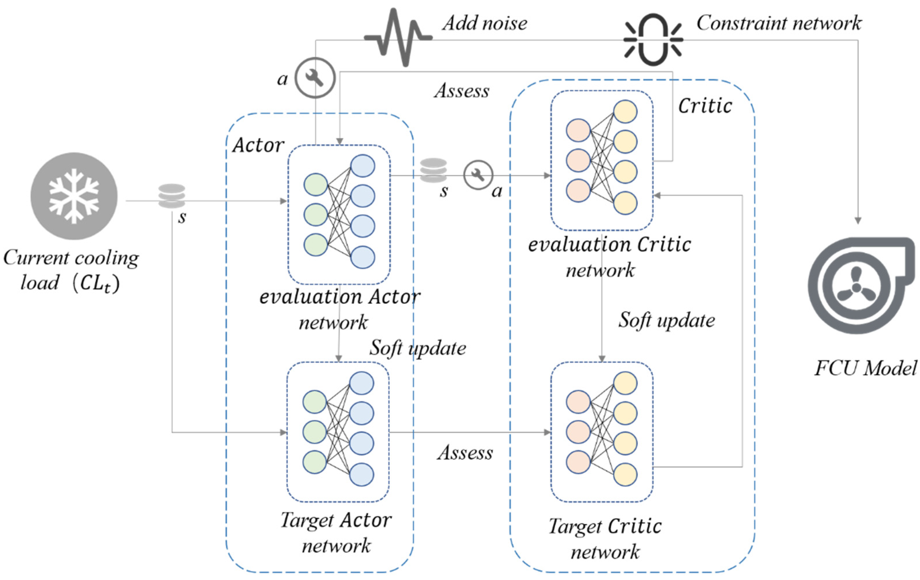
We end the current learning and go to Step 1. A dual neural network architecture (actor–critic network) is used in DDPG algorithm architecture, and a dual neural network model architecture (target-actor network and target-critic network) is used for both the policy function and the value function. Among them, the state ($C{L}_t$) is the input of DDPG, and the output actions interact with the environment and are stored in the experience replay pool. Figure 8 shows the control method based on FS-DDPG.

4.4. FS-DDPG Algorithm Based on SRL

In DDPG, the evaluation actor network belongs to the policy network, with the current state as input and the action as output; the action needs to have enough exploration; and we need to add noise $\mathcal{N}$. The action is shown in Equation (10):

$$\begin{array}{c}a=\mu \left(CL|{\theta }^{\mu }\right)+N\end{array}$$

(10)

where $a$ indicates the action taken by the agent, including $flo{w}_{water}$ and $flo{w}_{air}$. ${\theta }^{\mu }$ is the actor network parameter. $\mathcal{N}$ is a normally distributed noise; $\mu$ stands for the evaluation actor network. When an action $a$ is selected to act on the environment, the reward $r$ and the next state $s^{\prime }$ are subsequently obtained. At this time, experience samples $\left({s,a,r,s}^{\prime }\right)$ can be received and stored in the experience replay pool. When the samples in the experience replay pool reach the maximum capacity, the agent begins to learn and update the parameters of the network. Each time the network is updated, $N$ samples $(\left(s_i,a_i,r_i,s_{i+1}\right),iϵ\left(1,N\right))$ need to be drawn from the experience pool. The value function $Q$ is fitted through the critic network. The target $y_i=r_i+\gamma Q^{\prime }\left(s_{i+1},{\mu }^{\prime }\left(s_{i+1}\mid {\theta }^{{\mu }^{\prime }}\right)\mid {\theta }^{Q^{\prime }}\right)$ of each experience sample needs to be set to update the evaluation critic network. The loss function used to update the evaluation critic network is shown in Equation (11):

$$\begin{array}{c}L={\displaystyle \frac{1}{N}}{\sum }_i{\left(y_i-Q\left(s_i,a_i|{\theta }^Q\right)\right)}^2\end{array}$$

(11)

where $y_i$ represents the target value of sample $i$. $Q\left(s_i,a_i|{\theta }^Q\right)$ is the output of the evaluation critic network, which receives $s$ and $a$as inputs and outputs the corresponding action value function, where ${\theta }^Q$ represents the parameters of the evaluation critic network. Updates to the evaluation actor network are implemented through a policy gradient, as shown in Equation (12):

$$\begin{array}{c}{\left.{\left.{\nabla }_{{\theta }^{\mu }}\approx {\displaystyle \frac{1}{N}}{\displaystyle \sum _i} {\nabla }_{a}Q\left(s,a\mid {\theta }^Q\right)\right|}_{s=s_i,a=\mu \left(s_i\right)}{\nabla }_{{\theta }^{\mu }}\mu \left(s\mid {\theta }^{\mu }\right)\right|}_{s_i}\end{array}$$

(12)

where ${\nabla }_{a}Q\left(s,a\mid {\theta }^Q\right)$ is the gradient of the action value function $Q$ with respect to action $a$. This represents how the $Q$ function is adjusted to maximize the expected return in response to the action change. ${\nabla }_{{\theta }^{\mu }}\mu \left(s\mid {\theta }^{\mu }\right)$ represents the gradient of the actor function $\mu$ with respect to its parameter ${\theta }^{\mu }$.

Since the network $Q\left(s,a\mid {\theta }^Q\right)$ being updated is also used in calculating the target value, the $Q$ update is prone to divergence. As a result, the actor–critic was modified and updated with “soft” targets instead of copying weights directly. We create copies of the evaluation actor network $Q^{\prime }\left(s,a\mid {\theta }^{Q^{\prime }}\right)$ and the evaluation critic network $\mu \prime \left(s\mid {\theta }^{{\mu }^{\prime }}\right)$, respectively, to calculate the target values. These target networks then update their weights by their slow track of the learned network. The target networks are renewed in the form of soft updating paradigm, as shown in Equation (13).

$$\begin{array}{c}\begin{array}{c}\mathrm{update}\text{:}\left\{\begin{array}{c}{\theta }^{Q^{\prime }}\leftarrow \tau {\theta }^Q+\left(1-\tau \right){\theta }^{Q^{\prime }}\\ {\theta }^{{\mu }^{\prime }}\leftarrow \tau {\theta }^{\mu }+\left(1-\tau \right){\theta }^{{\mu }^{\prime }}\end{array}\right.\end{array}\end{array}$$

(13)

where ${\theta }^{Q^{\prime }}$ is the parameter of target critic network; ${\theta }^Q$ is the parameter of evaluation critic network; ${\theta }^{{\mu }^{\prime }}$ is the parameter of target actor network; and ${\theta }^{\mu }$ is the parameter of evaluation actor network. $\tau$ is the soft renewal coefficient. This means that the target values are constrained to change slowly, greatly improving the stability of learning.

As shown in the following algorithm, four networks are initialized at the beginning of the algorithm deployment. The initial assignment of network parameters follows a normal distribution to speed up the training process.

The agent accepts the room cooling load data and selects the action of water and air flow through the evaluation actor network. The reward is calculated by Equation (3), and a few moments later, we input the cooling load. We calculate the relative error in action output $∆a_t$ and progressively constrain the next action by $∆a_t$ in $r$. Based on the above interaction, the sample $\left(C{L}_t,flo{w}_{air},flo{w}_{water},r,C{L}_{t+1}\right)$ is collected into the experience replay pool. We draw $N$ experience samples from the experience replay pool.

For the network update, the evaluation critic network is updated by minimizing the mean square error between the actual value function and the estimated value function in batch experience. The evaluation actor network specifies the current policy by deterministically mapping states to a specific action. The evaluation actor network is updated through policy gradients.

In order to maintain the stability of the algorithm, the target network is updated by soft updating.

The following Algorithm 1 is an FCU control method based on the FS-DDPG algorithm.

Algorithm 1. The control method of an FCU based on FS-DDPG is presented.

$\mathrm{Randomly}\mathrm{initialize}\mathrm{critic}\mathrm{network}Q(s,a|{\theta }^Q)$$\mathrm{and}\mathrm{actor}\mu \left(s\right|{\theta }^{\mu })$$\mathrm{with}\mathrm{weights}{\theta }^Q$$\mathrm{and}{\theta }^{\mu }$. $\mathrm{Initialize}\mathrm{target}\mathrm{network}{Q}^{\prime }$$\mathrm{and}{\mu }^{\prime }$$\mathrm{with}\mathrm{weights}{\theta }^{Q\prime }\leftarrow {\theta }^Q$$,{\theta }^{{\mu }^{\prime }}\leftarrow {\theta }^{\mu }$ $\mathrm{Initialize}\mathrm{experience}\mathrm{replay}\mathrm{pool}R$ For episode = 1, M do $\mathrm{Initialize}\mathrm{a}\mathrm{random}\mathrm{process}$N for action exploration $\mathrm{Receive}\mathrm{initial}\mathrm{observation}\mathrm{state}{CL}_0$   For t = 1, to T do $\mathrm{Select}\mathrm{action}clip{(a}_t=\mu \left(s_t\right|{\theta }^{\mu })+{\mathcal{N}}_t,a_{min},a_{max})$$\mathrm{according}\mathrm{to}\mathrm{the}\mathrm{current}\mathrm{policy}\mathrm{and}$ $\mathrm{exploration}\mathrm{noise}{\mathcal{N}}_t$ # The selected action cannot exceed the limit value $\mathrm{Execute}\mathrm{action}{flow}_{water}$$\mathrm{and}{flow}_{air}$$\mathrm{and}\mathrm{reward}{r}_t$ and observe new $\mathrm{state}{CL}_{t+1}$ $\mathrm{Calculate}\mathrm{the}\mathrm{relative}\mathrm{error}\mathrm{in}\mathrm{action}\mathrm{output}∆a_t$$\mathrm{and}\mathrm{progressively}\mathrm{constraint}\mathrm{the}\mathrm{next}$ $\mathrm{action}\mathrm{by}∆a_t$$\mathrm{in}r$ # By calculating the relative error and constraining the    actions $\mathrm{Store}\mathrm{sample}({CL}_t,\left({flow}_{water},{flow}_{air}\right),r_t,{CL}_{t+1})$$\mathrm{in}R$ $\mathrm{Sample}\mathrm{a}\mathrm{random}\mathrm{minibatch}\mathrm{of}\mathrm{N}\mathrm{samples}$ $({CL}_{t,i},\left({flow}_{water,i},{flow}_{air,i}\right),r_{t,i},{CL}_{t+1,i})$$\mathrm{from}R$  $\mathrm{Set}{y}_i=r_i+\gamma Q^{\prime }(s_{i+1},\mu \prime (s_{i+1}\left|{\theta }^{\prime }\right)\left|{{\theta }^Q}^{\prime }\right)$    Update critic network by minimizing the loss function: $L={\displaystyle \frac{1}{N}}{\sum }_i{\left(y_i-Q\left(s_i,a_i|{\theta }^Q\right)\right)}^2$ Update the actor network using the sampled deterministic policy gradient:                             ${\nabla }_{{\theta }^{\mu }}J\approx {\displaystyle \frac{1}{N}}{\displaystyle \sum _i}{\nabla }_{a}Q(s,a{\left|{\theta }^Q)\right|}_{s=s_i,a=\mu \left(s_i\right)}{\nabla }_{{\theta }^{\mu }}\mu (s{\left|{\theta }^{\mu })\right|}_{s_i}$ Soft update the target networks: # Updating the target network by soft updating helps    to stabilize the training process $$\begin{gathered} \begin{array}{ll}{\theta }^{Q^{\prime }}& \leftarrow \tau {\theta }^Q+\left(1-\tau \right){\theta }^{Q^{\prime }}\\ \\ {\theta }^{{\mu }^{\prime }}& \leftarrow \tau {\theta }^{\mu }+\left(1-\tau \right){\theta }^{{\mu }^{\prime }}\end{array} \end{gathered}$$   End for End for

5. Experimental Results and Analysis

5.1. Experimental Parameter Setting

In the FS-DDPG control method based on SRL, there are four networks: the evaluation actor network, the evaluation critic network, the target actor network and the target critic network. The network structure of the evaluation actor is the same as that of the target actor, and the network structure of the evaluation critic is the same as that of the target critic.

Table 3. Network parameter setting.

Network	Number of Neurons	Activation Function	Learning Rate	Optimizer
Actor	1→64	ReLU	0.002	Adam
	64→2	Tanh
Critic	[1→64], [2→64]	ReLU	0.001	Adam
	64→1	ReLU

lists the structural parameters of the evaluation actor network and the evaluation critic network.

The exploration degree exponentially decays the standard deviation of a normal distribution.

$$\begin{array}{c}{\sigma }_t=var\times k_{var}\end{array}$$

(14)

where ${\sigma }_t$ is the standard deviation in time step $t$, $var$ is the initial standard deviation, and after a single execution, the standard deviation ${\sigma }_t$ becomes $k_{var}$ multiplied by the initial value $var$, where $k_{var}$ is less than 1. As time goes by, the standard deviation index decreases, the control method gradually becomes stable. To ensure that the algorithm maintains a certain learning rate in the later stages, the minimum $va{r}_{min}$ is set to 0.15. In CMDP, there is a greater focus on a short period of benefits, so the discount factor $\gamma$ is set to 0.01. For updating the target networks, a soft update method is used, with a soft update coefficient $\tau$ also set to 0.01. The specific hyperparameters are detailed in

Table 4. Hyperparameter setting.

Hyperparameter	Value
Soft renewal coefficient $\tau$	0.01
Replay pool size	2000
Sample batch size	64
Discount factor $\gamma$	0.01
Standard deviation minimum $va{r}_{min}$	0.15
Standard deviation decay $k_{var}$	0.995

.

5.2. Experimental Comparison Method

The experiment for the FCU system control method based on FS-DDPG primarily involves comparisons with RBC, MBC, DQN and control methods based on DDPG.

• DDPG control method: DDPG is a widely used DRL algorithm in continuous action spaces. The advantage of DDPG lies in its ability to automatically adjust control strategies through training, without relying on manually designed rules. However, DDPG tends to exhibit significant action fluctuations in high-dynamic environments, which can compromise equipment safety, reduce energy efficiency and fail to meet practical application requirements. By comparing with DDPG, FS-DDPG can clearly demonstrate significant advantages in reducing flow fluctuations, improving energy efficiency and enhancing control performance. It also proves its effectiveness in addressing the safety issues present in real-world applications. Apart from the strategy constraint optimization, the network parameters in DDPG are the same as those in the FS-DDPG control method.
• MBC control method: In practice, it is usually difficult to obtain an accurate FCU model. Moreover, the MBC method here is obtained by exhaustively enumerating all control nodes of FCU. This method obtains the optimal solution from the global perspective, but it consumes a lot of computing resources and lacks dynamic adaptability. Adopting this method, the gap between the FS-DDPG method and the optimal method can be reflected. The objective function for this method is provided in Equation (15):

  $$\begin{array}{c}J\left(flo{w}_{air},flo{w}_{water}\right)=-k\left(1-e^{-{\displaystyle \frac{{\left(Q_{FCU}-CL\right)}^2}{2\times {\left(0.1\times CL\right)}^2}}}\right)-\left(P_{pump}+P_{fan}\right)\end{array}-k\ast diff$$

  (15)

  where $flo{w}_{air}$ and $flo{w}_{water}$ are the independent variables. $Q_{FCU}$, $P_{pump}$ and $P_{fan}$ can be calculated through ${flow}_{air}$ and ${flow}_{water}$. $diff$ represents the relative error in the actions of the fan and pump before and after. By maximizing the function $J(flo{w}_{air},flo{w}_{water})$ through a traversal method, the optimal water flow and air flow for each state are determined.

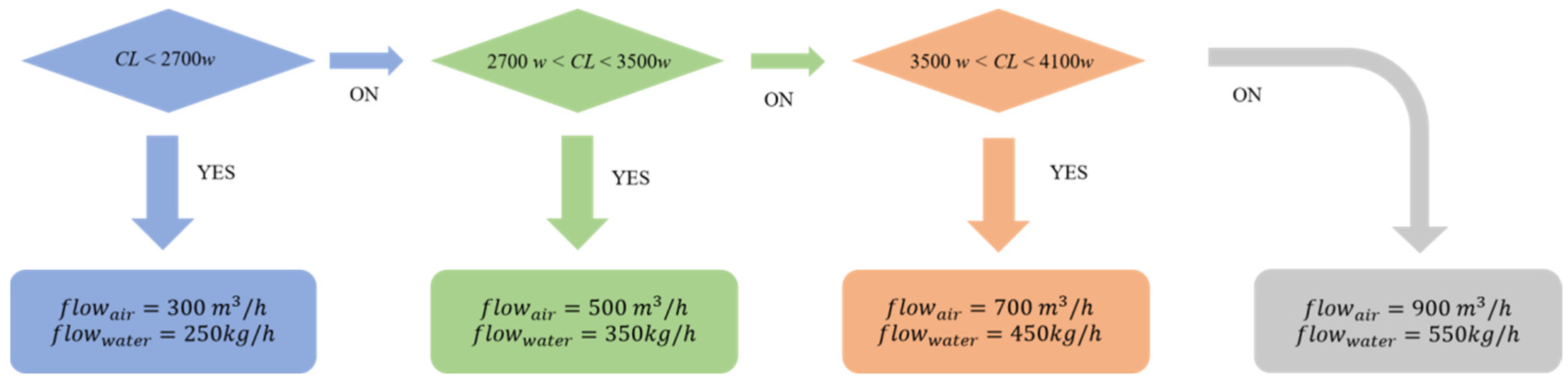
• RBC control method: RBC is a traditional control method that typically adjusts system control parameters based on experience and rules. The RBC method is simple and intuitive, performing well in static or relatively stable environments. However, when facing dynamic changes in the environment, RBC often requires frequent rule adjustments, which is not feasible in complex or uncertain systems. Additionally, RBC has a limited capability in optimizing system energy consumption. In contrast to RBC, FS-DDPG demonstrates its advantages in dynamic environments, particularly in significantly improving system energy efficiency and control accuracy. According to expert experience, the RBC control method is implemented through sequential decision-making, as shown in Figure 9.
• The control logic for this sequential decision is as follows: When $CL\mathsf{ϵ}\left(\mathrm{0,2700}\right)$, set $flo{w}_{air}=300{\mathrm{m}}^3/\mathrm{h}$ and $flo{w}_{water}=250\mathrm{k}\mathrm{g}/\mathrm{h}$; when CL $CL\mathsf{ϵ}\left(\mathrm{2700,3500}\right)$, set $flo{w}_{air}=500{\mathrm{m}}^3/\mathrm{h}$ and $flo{w}_{water}=350\mathrm{k}\mathrm{g}/\mathrm{h}$; when $CL\mathsf{ϵ}\left(\mathrm{3500,4100}\right)$, set $flo{w}_{air}=700{\mathrm{m}}^3/\mathrm{h}$ and $flo{w}_{water}=450\mathrm{k}\mathrm{g}/\mathrm{h}$; when $CL\mathsf{ϵ}(4100,\mathrm{\infty })$, set $flo{w}_{air}=900{\mathrm{m}}^3/\mathrm{h}$ and $flo{w}_{water}=550\mathrm{k}\mathrm{g}/\mathrm{h}$.
• DQN control method: In MDP modeling, the setting of state, action and reward is the same as that of DDPG. The value range of water flow for pump is 80–700 kg/h, and the step size is 5 $\mathrm{k}\mathrm{g}/\mathrm{h}$. The value range of air flow for fan is 100–1200 m³/h, and the step size is 5 m³/h. The policy network and target network of the agent are composed of two hidden layers containing 32 neurons. The training batch $batch\_size$ is set to 32, and the discount factor $\gamma$ is set to 0.01. The update step $C_{step}$ is set to 200; the learning rate is set to 0.01; and the experience pool capacity $D$ is set to 2000. Detailed parameter settings are shown in

  Table 5. DQN hyperparameter settings.

  Hyperparameter	Value
  Neurons in hidden layers	32, 32
  Sample batch size	32
  Discount factor $\gamma$	0.01
  Learning rate	0.001
  Replay pool size $D$	2000
  Update step $C_{step}$	200
  Training round $Episodes$	20

  .

In summary, RBC is suitable for simple scenarios without dynamic adjustment, but lacks flexibility and optimization capabilities; MBC is suitable for systems with accurate models and can provide optimal control effects, but it requires high-quality models and data. DDPG and FS-DDPG are more suitable for dynamically changing complex systems, and FS-DDPG further improves the robustness of the FCU control process. DQN performs well in discrete action spaces and is capable of handling relatively less complex systems, but it struggles with stability in highly dynamic environments due to its reliance on a value-based approach and limited exploration–exploitation balance.

5.3. Experimental Results

In order to evaluate the performance of the proposed algorithm, we present the analysis of algorithm convergence, energy consumption analysis, system operational performance analysis, system safety analysis and satisfaction analysis. In terms of room layout, temperature and humidity, insulation and other aspects, room 1-N-6 is typical of all rooms, so choosing room 1-N-6 for experiments can ensure the universality of the algorithm.

5.3.1. Analysis of Algorithm Convergence

Figure 10 presents the trend of cumulative rewards over a decade using the FS-DDPG and DDPG control methods, where the abscissa is the year in the training process, and the ordinate is the reward value. The solid line in Figure 10 represents the average reward value of the 10 independent experiments, and the shadow represents the error band in the 10 experiments, where the green is the experimental result under FS-DDPG, and the blue is the experimental result of DDPG. In DRL, the trend of cumulative reward can indicate the convergence of the algorithm, and the reward reflects the effectiveness of the control to some extent. As can be seen from Figure 10, both the DDPG and FS-DDPG methods initially exhibit wide error bands. With the optimization of the algorithm, the error band is gradually narrowed. Around the fifth year, the reward value converges; by the end of the eighth year, the error band basically converges, which indicates that both DDPG and FS-DDPG can converge. At the end of training, the reward value of FS-DDPG was slightly higher than that of DDPG, which also indicated that the control effect of FS-DDPG was better.

Furthermore, FS-DDPG is a model-free RL algorithm, and once the system converges and stabilizes, the control parameters will stabilize as well. Compared to traditional methods, FS-DDPG can reduce equipment wear and maintenance needs. If the system needs adjustments in the future, re-training the model is sufficient, without additional equipment maintenance. This enables FS-DDPG to effectively reduce maintenance costs and extend equipment lifespan during long-term operation.

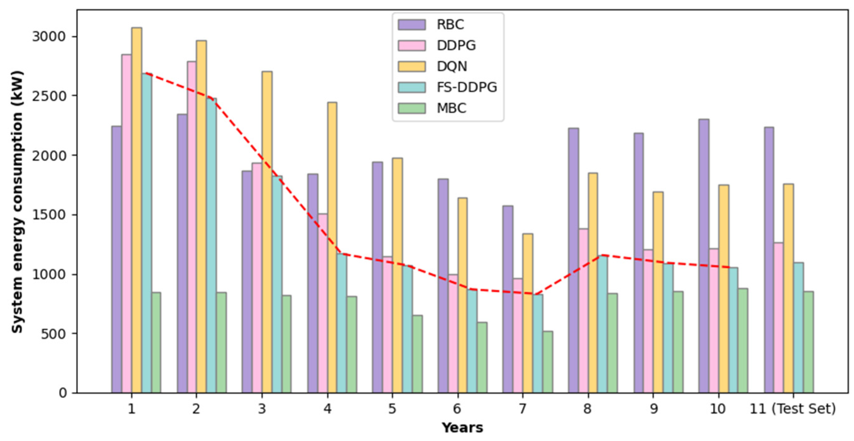
5.3.2. Energy Consumption Analysis

Figure 11 shows the average energy consumption of the five control methods based on 10 independent experiments, where the abscissa is the years, and the ordinate is the system energy consumption. As can be seen from the red curve in Figure 11, with the progress of training, the total energy consumption of the system under the control of FS-DDPG has a huge reduction. In the first two years, the energy consumption of FS-DDPG and DDPG was higher than that of RBC. However, after the optimization of the algorithm, the energy consumption of FS-DDPG in the test set was 1080.75 kWh, and compared with DDPG, RBC and DQN, the energy saving rate reached 11.90%, 51.76% and 37.61%, respectively. Compared with DQN, FS-DDPG demonstrates more significant energy savings. While DQN performs well in systems with discrete action spaces, it struggles in highly dynamic environments, leading to less efficient control and higher energy consumption in comparison to FS-DDPG. Therefore, the results prove that the application of FS-DDPG has a positive effect on the energy saving control of FCU. With the respect to the total energy consumption, compared with MBC (the optimal control method), FS-DDPG and DDPG have a similar energy saving performance. But, from the 1st year to the 10th year, FS-DDPG outperforms DDPG all of the time, where the reason is that, for all fluctuating action points, FS-DDPG allows for better consistency in the water and air flow of the system and lower energy consumption in practical applications.

In addition, we conducted the experiment using a separate test set (NOAA 2022 weather data) [27], representing a real test scenario, the results of which can be seen in Year 11 (test set). It can be seen from Figure 11 that the experimental results of the test set are very close to the energy consumption of the 9th and 10th years, which indicates that the performance improvement achieved in the training process is not only limited to the training set, but also applies to the new data. Test set experiments help to address potential problems of overfitting simulated environments.

Table 6. Energy consumption confidence interval analysis (CI) for different methods across 10 years.

Year	Energy Consumption Confidence Interval Analysis (kWh)
	RBC	DDPG	DQN	FS-DDPG	MBC
1	(2030.85, 2450.54)	(2743.08, 2955.51)	(3062.25, 3274.68)	(2482.97, 2890.17)	(814.68, 872.57)
2	(2362.05, 2851.11)	(2457.47, 2691.95)	(2843.67, 3078.15)	(2258.52, 2699.19)	(812.85, 876.83)
3	(1692.23, 2046.08)	(1832.25, 2025.76)	(2594.17, 2807.03)	(1739.33, 1916.79)	(795.48, 852.10)
4	(1654.64, 2025.36)	(1399.21, 1618.03)	(2323.62, 2564.32)	(1113.18, 1221.68)	(778.72, 838.32)
5	(1641.67, 2241.42)	(1008.48, 1289.48)	(1841.49, 2122.49)	(1003.07, 1144.15)	(622.35, 690.82)
6	(1489.11, 2112.28)	(982.09, 1253.88)	(1495.38, 1794.35)	(864.03, 1024.02)	(561.55, 628.13)
7	(2407.06, 2845.89)	(880.16, 1036.82)	(1198.10, 1485.62)	(783.36, 909.26)	(496.16, 547.21)
8	(2015.07, 2442.22)	(1150.62, 1404.40)	(1706.29, 1985.44)	(1040.31, 1271.24)	(812.83, 865.38)
9	(2083.30, 2510.34)	(1117.06, 1295.12)	(1590.59, 1786.45)	(964.74, 1113.13)	(828.22, 884.86)
10	(2281.93, 2668.55)	(1104.88, 1315.05)	(1642.64, 1852.81)	(925.97, 1034.22)	(851.87, 902.40)

shows the confidence interval for energy consumption (kWh) of the five methods in each year. The confidence interval (CI) is calculated as shown in Equation (16):

$$CI=\mu \pm Z\ast {\displaystyle \frac{SD}{\sqrt{n}}}\#$$

(16)

where $SD$ is the standard deviation, $n$ is the amount of data per year and $Z$ is the Z-value of the 95% confidence interval, usually taken as 1.96.

As training progresses, the energy consumption confidence interval of FS-DDPG narrows overall, demonstrating a significant improvement in the stability of its performance. The confidence interval of FS-DDPG is consistently smaller than that of DQN, DDPG and RBC, with a notable example in the tenth year: the intervals for FS-DDPG, DDPG, RBC and DQN are (925.97, 1034.22), (1104.88, 1315.05), (2281.93, 2668.55) and (1642.64, 1852.81), respectively. This indicates that FS-DDPG performs more effectively in reducing energy consumption.

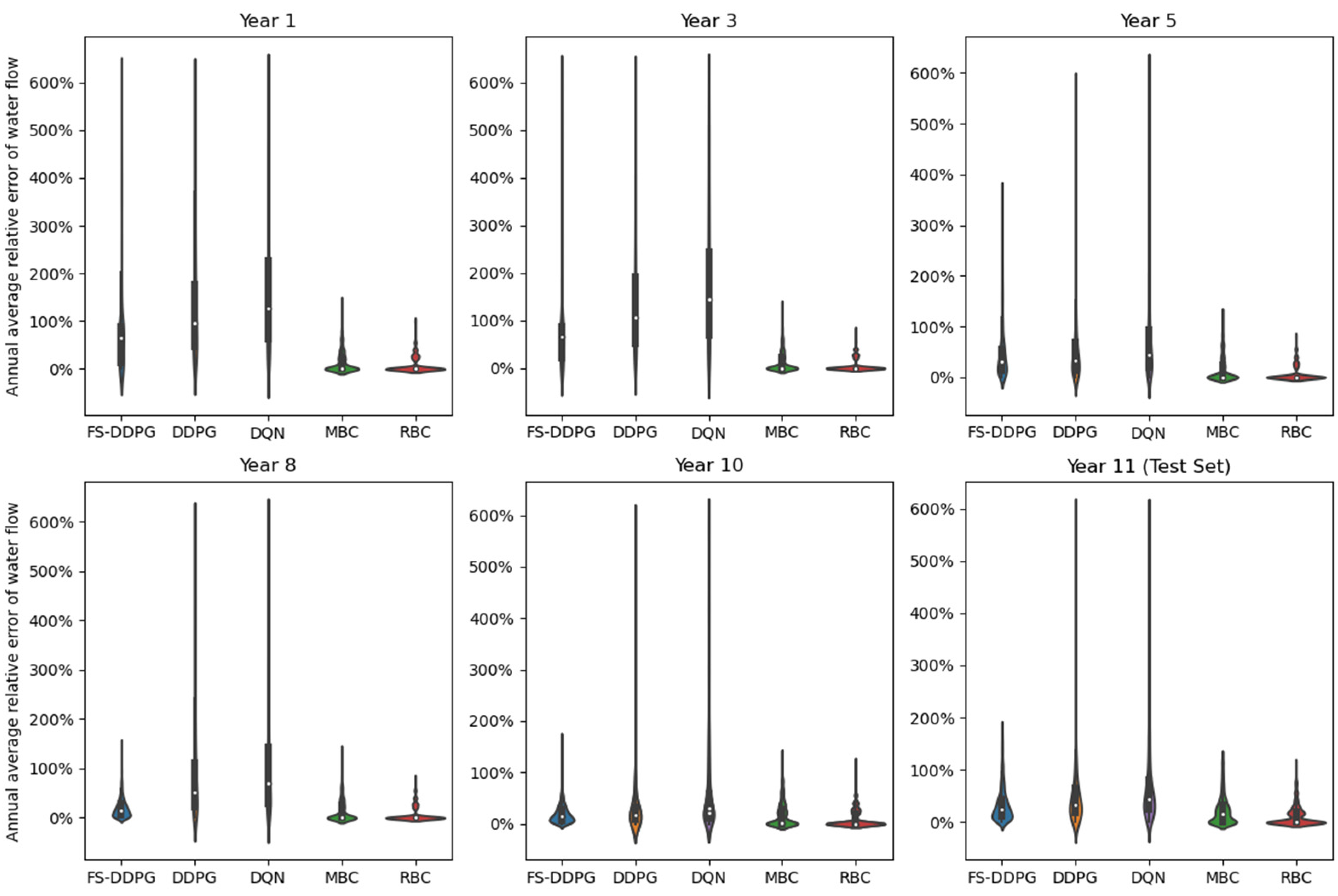
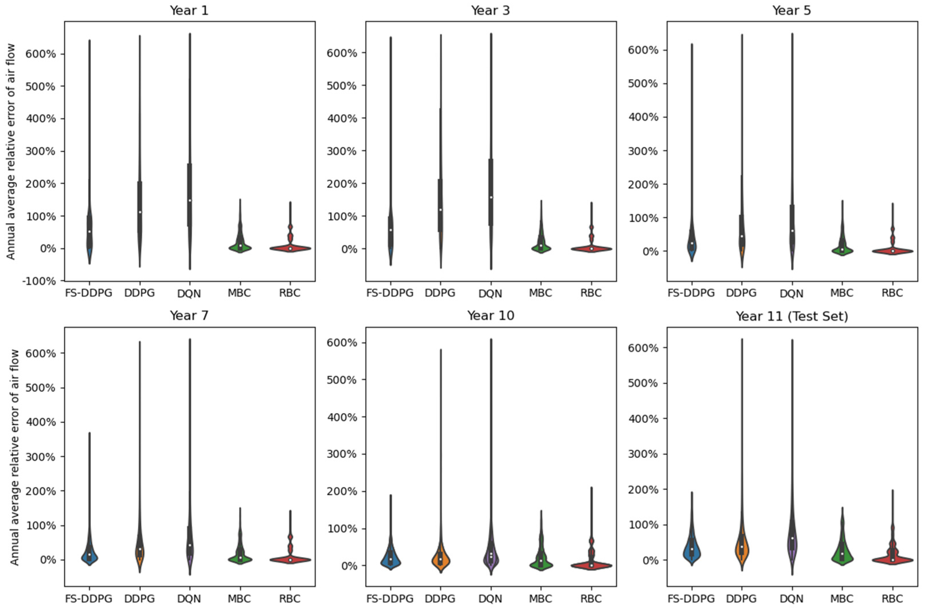
5.3.3. System Operation Performance Analysis

With the progress of training, FS-DDPG and DDPG are approaching the optimal control method. We describe this process in terms of the relative error $G$. The calculation equation of relative error $G$ is as shown in Equation (17):

$$\begin{array}{c}G={\displaystyle \frac{\left|a-a^{\prime }\right|}{a^{\prime }}}\ast 100\%\end{array}$$

(17)

where $a$ is the output water flow under FS-DDPG or DDPG, and $a\prime$ is the output water flow under MBC.

Figure 12 shows the annual average relative error distribution of FS-DDPG, DDPG and MBC in water flow control, with the vertical axis representing the relative error (%). By selecting specific years for comparison, it can be observed that the distribution of annual average relative errors in water flow varies significantly. The blue and orange squares represent most of the normal relative error distribution, indicating that FS-DDPG, DDPG and MBC have similar effects in controlling water flow. The gray dots above the upper edge (horizontal line) represent outliers, indicating that DDPG, FS-DDPG and MBC have obvious differences in the control effect. During the learning process, $G$ become more concentrated and smaller, which indicates that the control effect of these two algorithms moves closer and closer to MBC in general. And the outliers in the $G$ between FS-DDPG and MBC are decreasing, indicating that the selected action of FS-DDPG could be closer to MBC. On the contrary, although $G$ between DDPG and MBC becomes smaller and concentrated, there are still many outliers at the end of training. This situation indicates that there is still a big gap between DDPG and MBC in water flow control, which is mainly caused by the lack of constraint on fluctuation action in DDPG.

Where $\mathrm{a}$ is the output air flow under FS-DDPG or DDPG, and $a_{MBC}$ is the output air flow under MBC.

Figure 13 shows the annual average relative error distribution of FS-DDPG, DDPG and MBC in air flow control, with the vertical axis representing the relative error (%). By selecting specific years for comparison, it can be observed that the distribution of annual average relative errors in air flow varies significantly. The blue and orange squares represent most of the normal relative error distribution, indicating that FS-DDPG, DDPG and MBC have similar effects in controlling air flow. The gray dots above the upper edge (horizontal line) represent outliers, indicating that DDPG, FS-DDPG and MBC have obvious differences in the control effect. During the learning process, $G$ become more concentrated and smaller, which indicates that the control effect of these two algorithms moves closer and closer to MBC in general. And the outliers in the $G$ between FS-DDPG and MBC are decreasing, indicating that the selected action of FS-DDPG could be closer to MBC. On the contrary, although $G$ between DDPG and MBC becomes smaller and concentrated, there are still many outliers at the end of training. This situation indicates that there is still a big gap between DDPG and MBC in air flow control, which is mainly caused by the lack of constraint on fluctuation action in DDPG.

Additionally, when the relative error of water or air flow $\left(G\right)$ is less than 0.5, it is considered to satisfy the action consistency (AC). The formula for calculating action consistency is as follows:

$$AC={\displaystyle \frac{{Amount}_{consistentaction}}{{Amount}_{totalaction}}}\ast 100\%\#$$

(18)

where ${Amount}_{consistentaction}$ represents the amount of water or air flow set points in a year that satisfy the action consistency condition, and ${Amount}_{totalaction}$ represents the total amount of water or air flow set points in that year.

Table 7. Annual water and air flow action consistency analysis.

Year	AC
	Water Flow		Air Flow
	DDPG	FS-DDPG	DDPG	FS-DDPG
1	45.00%	46.13%	39.87%	41.60%
2	45.66%	46.03%	42.95%	43.74%
3	48.93%	52.52%	44.12%	48.09%
4	57.10%	71.43%	57.11%	59.76%
5	73.72%	83.99%	73.43%	74.79%
6	84.78%	86.41%	84.46%	87.44%
7	83.66%	86.74%	85.65%	90.48%
8	82.77%	85.15%	83.97%	84.78%
9	83.34%	88.70%	85.03%	88.71%
10	83.74%	89.96%	86.59%	89.23%

shows the annual water and air flow action consistency analysis. As shown in Table 7, FS-DDPG shows a year-on-year improvement in action consistency for both water flow and air flow control. In terms of water flow, FS-DDPG reaches 89.96% in the tenth year, a significant improvement compared to DDPG’s 83.74%. For air flow, FS-DDPG also outperforms DDPG, with an action consistency of 89.23% in the tenth year, while DDPG stands at 86.59%. This indicates that FS-DDPG performs better than DDPG in terms of control accuracy and consistency for both water and air flows, showing results closer to the control performance of MBC.

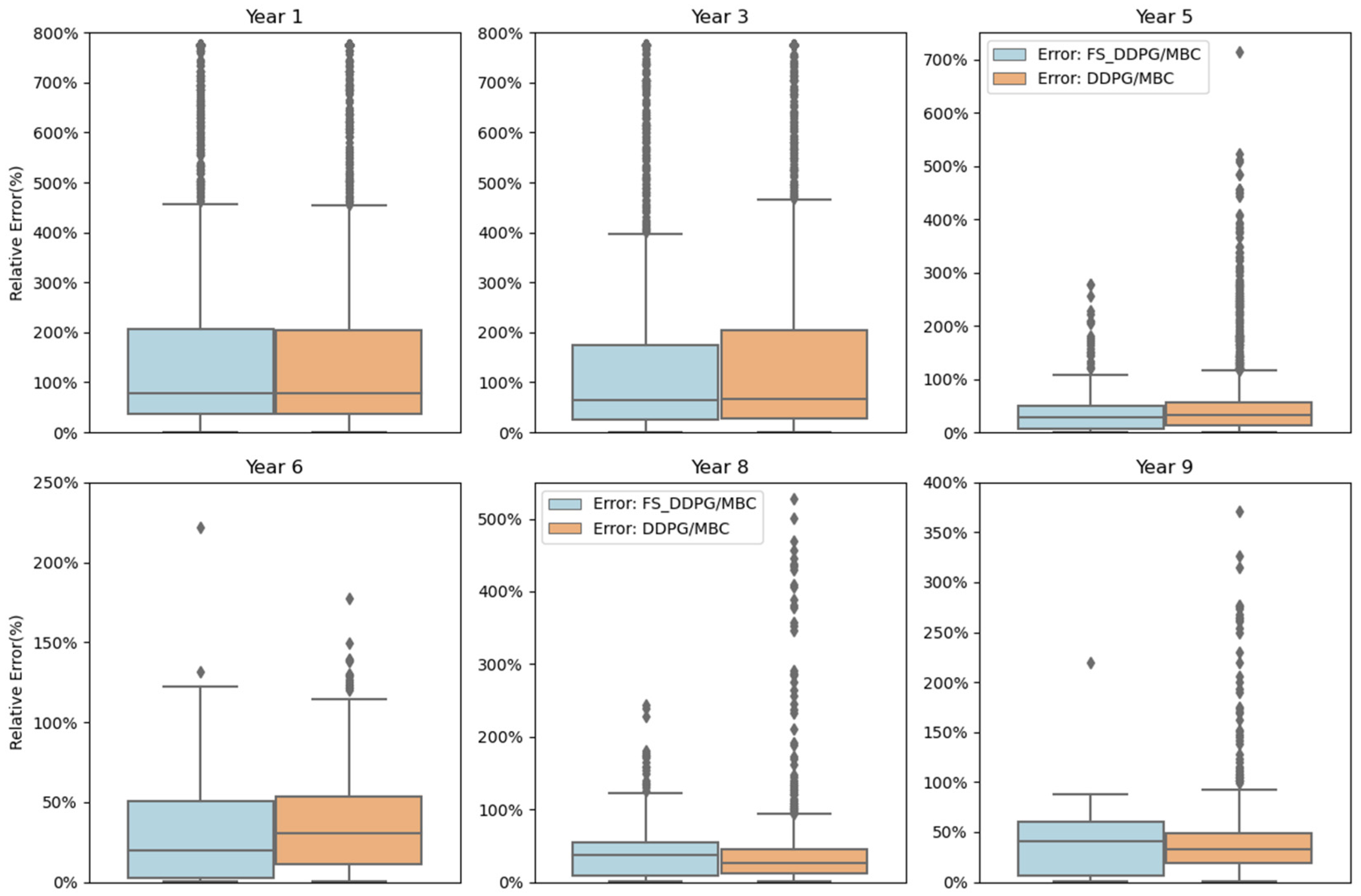
5.3.4. System Safety Analysis

By comparing the changes between annual average water flow relative errors across different years, we try to analyze the performance of system stability for five control methods. The relative error is calculated in Equation (17), where $a$ is $a_t^{water}$, $a^{\prime }$ is $a_{t-1}^{water}$. $a_t^{water}$ is the water flow of the system at moment $t$ and $a_{t-1}^{water}$ is the water flow of the system at moment $t-1$. Figure 14 presents the annual average relative error distribution in water flow for the five control methods: FS-DDPG, DDPG, MBC, DQN and RBC, based on some selected years, showing significant changes in the relative error of average water flow. The abscissa is the five methods, and the vertical axis is the annual average relative error of the water flow (%). In the first year, for MBC and RBC, most of the values concentrate near zero. The reason is that MBC is the optimal control method, and RBC is a rule-based control method. For DDPG, DQN and FS-DDPG, the error value distribution is relatively scattered (between 0 and 650%) while partial actions exist with considerable error values. The reason is that the agent has selected actions with significant differences before and after. As training progresses, the outliers (large error values) for FS-DDPG gradually decrease (the error values of FS-DDPG gradually converge towards zero), which indicates that FS-DDPG’s constraints on action fluctuations are increasingly effective. However, the error value distribution for DDPG and DQN remains dispersed, with some actions exhibiting considerable variability (such as the error distribution of DDPG ranging from 0 to 620% in the 10th year). At the end of the training, the FS-DDPG graph approaches that of MBC and RBC (the error values of FS-DDPG are concentrated between 0 and 1.8), while there is no significant change in the DDPG and DQN. In the test set, FS-DDPG reduced the dramatic fluctuations of water flow ($G$ > 1) by 98.20% compared to DDPG. This indicates that there are no constraints on fluctuating actions in DDPG, which also demonstrates that constraints on actions are helpful for the algorithm to converge to a thorough strategy.

In addition, to ensure the robustness of the results, we conducted the experiment using a separate test set (NOAA 2022 weather data) [27] representing a real test scenario, the result of which can be seen in Year 11 (test set). By comparing the subgraphs, it can be found that the distribution of water flow error range in the test set closely aligned with the distribution of the 8th and 10th years, which indicates that the performance improvements achieved during training are not limited to the training set, but also apply to new data. By incorporating Year 11 as a test set, we address potential concerns of overfitting to the simulated environment and strengthen the applicability of the proposed control methods to real-world scenarios.

By comparing the changes between annual average air flow relative errors across different years, the performance of the five control method in terms of system stability can be analyzed, where $a$ is $a_t^{air}$, $a^{\prime }$ is $a_{t-1}^{air}$ and $a_t^{air}$ is the air flow of the system at moment $t$, $a_{t-1}^{air}$ is the air flow of the system at moment $t-1$. Figure 15 presents the annual average relative error distribution in air flow for the five control methods: FS-DDPG, DDPG, MBC, DQN and RBC, based on some selected years, showing significant changes in the relative error of average air flow. The abscissa is the five methods, and the vertical axis is the annual average relative error of the air flow (%). In the first year, for MBC and RBC, most of the values concentrate near zero. The reason is that MBC is the optimal control method, and RBC is a rule-based control method. For DDPG, DQN and FS-DDPG, the error value distribution is relatively scattered (between 0 and 650%) while partial actions exist with considerable error values. The reason is that the agent has chosen actions with significant differences before and after. As training progresses, the outliers (large error values) for FS-DDPG gradually decrease (the error values of FS-DDPG gradually converge towards zero), which indicates that FS-DDPG’s constraints on action fluctuations are increasingly effective. However, the error value distribution for DDPG and DQN remains dispersed, with some actions exhibiting considerable variability (such as the error distribution of DDPG ranging from 0 to 630% in the 10th year). At the end of the training, the FS-DDPG graph approaches that of MBC and RBC (the error values of FS-DDPG are concentrated between 0 and 1.9), while there is no significant change in the DDPG and DQN graphs. In the test set, FS-DDPG had reduced the dramatic fluctuations of air flow ($G$ > 1) by 95.82% compared to DDPG. This indicates that there were no constraints on fluctuating actions in DDPG, which also demonstrates that constraints on actions are helpful for the algorithm to converge to a thorough strategy.

In addition, to ensure the robustness of the results, we conducted the experiment using a separate test set (NOAA 2022 weather data) [27] representing a real test scenario, the result of which can be seen in Year 11 (test set). By comparing the subgraphs, it can be found that the distribution of air flow error range in the test set closely aligned with the distribution of the 7th and 10th years, which indicates that the performance improvements achieved during training are not limited to the training set, but also apply to new data. By incorporating Year 11 as a test set, we address potential concerns of overfitting to the simulated environment and strengthen the applicability of the proposed control methods to real-world scenarios.

Table 8. Comparison of DDPG and FS-DDPG in the fluctuation of water flow and air flow.

Year	$\mathbf{The}\mathbf{Amount}\mathbf{of}\mathbf{Fluctuating}\mathbf{Flow}(\mathit{G}$ > 1)
	Water Flow			Air Flow
	DDPG	FS-DDPG	Reduced Proportion	DDPG	FS-DDPG	Reduced Proportion
1	1038	496	52.22%	1092	525	52.04%
2	1136	487	57.13%	1095	571	47.89%
3	1184	539	54.48%	1135	551	51.47%
4	735	447	39.18%	882	483	45.29%
5	472	172	63.56%	530	237	55.66%
6	359	61	83.01%	464	133	71.32%
7	366	57	84.43%	363	79	78.25%
8	640	9	98.59%	712	28	96.07%
9	595	4	99.33%	677	18	97.34%
10	430	11	97.44%	538	26	95.17%
11 (Test Set)	557	10	98.20%	645	27	95.82%

shows the comparison between DDPG and FS-DDPG control methods in the fluctuation of water flow and air flow. By calculating the reduction proportion of fluctuating flow for FS-DDPG compared to DDPG, it reflects the stability advantage of FS-DDPG in the control process. Particularly in the later years, FS-DDPG shows a significant advantage in reducing fluctuations. In the test set, compared to DDPG, FS-DDPG reduced water flow fluctuations by 98.20% and air flow fluctuations by 95.82%. These results indicate that FS-DDPG can more effectively and smoothly control the system, reducing extreme fluctuations.

5.3.5. Satisfaction Analysis

In the FCU system, it is crucial to maintain consistency between the real cooling capacity and the required cooling load. We use the cooling load deviation to represent the relationship between real cooling capacity and required cooling load, as shown in Equation (19):

$$\begin{array}{c}\Delta CL=|{CL}_t^{FCU}-C{L}_t|\end{array}$$

(19)

where $\Delta CL$ represents the cooling load deviation at moment $t$, ${CL}_t^{FCU}$ is the cooling capacity at moment $t$ and $C{L}_t$ is the expected cooling load at moment $t$. We use the daily cooling load deviation to validate the FCU system’s ability of meeting during the cooling season over ten years. Figure 16 shows the cooling load deviation in selected six years (these six years have evident cooling load deviations), where the abscissa is the number of days in the cooling season and the ordinate is the time (only considering human activity time: 7:00–21:00). Lighter-colored areas indicate smaller cooling load deviations, while darker-colored areas indicate larger deviations. In the first year, it can be clearly found that there are many dark squares with large $\Delta CL$ values, which represent large deviations between actual cooling capacities and expected cooling loads. During the learning process, the number of dark squares gradually decreases, which not only indicates that the time period with a large cooling load deviation is decreasing, but also reflects that FS-DDPG is constantly optimized and finally shows a good performance. However, in all ten years, there are still some dark-colored squares. The presence of these dark areas indicates that the system is unable to fully meet the cooling load requirements at certain moments, which may be related to external climatic conditions, internal load fluctuations or system maintenance.

Table 9. The variation trend of the annual satisfaction rate of 5 methods.

Year	SR
	DDPG	FS-DDPG	RBC	MBC	DQN
	DDPG	FS-DDPG	DDPG	FS-DDPG
1	15.51%	17.13%	58.19%	92.89%	12.84%
2	26.72%	25.02%	59.34%	93.45%	22.83%
3	37.67%	38.52%	60.04%	93.24%	28.34%
4	46.94%	49.43%	59.48%	92.96%	39.12%
5	65.79%	70.99%	59.12%	92.67%	53.64%
6	74.78%	77.41%	59.79%	94.11%	59.79%
7	78.66%	83.74%	60.51%	92.82%	68.51%
8	84.17%	85.15%	58.96%	93.05%	71.96%
9	83.34%	83.16%	59.22%	94.25%	70.22%
10	84.74%	84.706%	60.16%	92.74%	72.16%
11 (Test Set)	84.18%	84.33%	59.77%	93.46%	69.77%

shows the trend of the satisfaction rate (SR) for each method. The satisfaction rate is calculated in Equation (20):

$$SR={\displaystyle \frac{{Satisfield}_{hours}}{{total}_{hours}}}\ast 100\%\#$$

(20)

where ${total}_{hours}$ presents the total hours in a year and ${Satisfield}_{hours}$ represents the number of hours in which the cooling load demand is met. When $\Delta CL$ is less than 10% of $C{L}_t$, it is considered to meet the current actual cooling capacity demand.

5.3.6. Sensitivity Analysis

In order to further evaluate the stability of the control strategy and system performance, we perform sensitivity analysis on several key parameters using the test set, focusing on the change in penalty term weights and constraint tightening thresholds. We adjusted the values of these parameters and analyzed their impact on system performance.

Table 10. Performance comparison of FS-DDPG with different penalty term weights and constraint tightening thresholds.

$\mathbf{Penalty}\mathbf{Term}\mathbf{Weights}\mathit{\lambda }$	$\mathbf{Constraint}\mathbf{Tightening}\mathbf{Thresholds}\mathit{\beta }$	Satisfaction Rate (SR)	Energy Consumption	Fluctuation Reduction Ratio (Compared to DDPG)
				Water flow	Air flow
10.0	1.0	84.33%	1080.75 kWh	98.20%	95.82%
5.0	1.0	84.22%	1157.91 kWh	84.18%	76.69%
15.0	1.0	82.35%	1201.93 kWh	99.57%	98.81%
10.0	0.5	82.17%	1278.47 kWh	99.83%	99.15%
10.0	2.0	83.94%	1137.62 kWh	65.72%	59.09%

is a performance comparison of FS-DDPG with different penalty term weights and constraint tightening thresholds. In all the tested combinations in Table 7, FS-DDPG performs best when the penalty term weight is 10.0 and the constraint tightening threshold is 1.0. In this case, the fluctuation reduction ratios for water flow and air flow are 98.2% and 95.82%, respectively, with an energy consumption of 1080.75 kWh and a satisfaction rate (SR) of 84.33%. In contrast, other combinations generally show higher energy consumption and lower satisfaction rates. Specifically, when the penalty term weight increases ($\lambda =15)$ or the constraint tightening threshold decreases ($\beta =0.5)$, the fluctuation reduction ratio remains relatively constant, but both energy consumption and the satisfaction rate worsen. This is because the agent tends to choose more conservative actions, sacrificing energy efficiency and satisfaction to ensure smoother actions. Overall, the combination of a penalty term weight of 10.0 and a constraint tightening threshold of 1.0 achieves the best balance between satisfaction rate, energy saving and safety performance.

6. Conclusions and Future Work

When traditional RL methods are applied to control the FCU, significant flow fluctuations may occur, leading to system overload, increased energy consumption and even equipment damage. To address this challenge, we model the FCU control process as a constrained Markov decision process, limiting the agent’s action space by incorporating a penalty term for process constraints within the reward function. Based on this, we propose the FS-DDPG algorithm based on SRL to optimize the control strategy for FCU. To validate the performance of the proposed algorithm, we utilized DeST software to construct a model of office rooms based on real historical weather data and calculate the corresponding cooling load demand. A heat and mass transfer model for the FCU was established, effectively validating the accuracy and feasibility of the model. The experimental results show the following:

• Compared with DDPG, FS-DDPG can suppress 98.20% of pump flow fluctuations and 95.82% of fan airflow fluctuations. Additionally, compared with RBC and DDPG, FS-DDPG achieves energy savings of 11.9% and 51.76%, respectively.
• The proposed method shows performance and satisfaction levels very close to those of MBC, indicating that FS-DDPG is highly adaptable to dynamic environments, able to meet the indoor cooling load requirements, reduce system energy consumption and ensure long-term stable operation of the system.

In the early stages of the learning process, due to the exploration mechanism of the algorithm and dynamic changes in the environment, there are still some large fluctuations in water and air flow. The Lyapunov method may offer a solution, but balancing stable system operation with efficiency remains challenging. This will be a focus for future research. Furthermore, in future studies, we plan to further extend the FS-DDPG method to explore its application in more complex and variable FCU systems, especially for multi-region FCU systems. At the same time, we will also consider the performance of the system in different environments, especially how to ensure the balance between system stability and energy efficiency under abnormal conditions or uncertain factors.

References

1. Ding, Z.K.; Fu, Q.M.; Chen, J.P.; Wu, H.J.; Lu, Y.; Hu, F.Y. Energy-efficient control of thermal comfort in multi-zone residential HVAC via reinforcement learning. Conn. Sci. 2022, 34, 2364–2394. [Google Scholar] [CrossRef]
2. World Energy Outlook 2023. Available online: www.iea.org/terms (accessed on 8 January 2025).
3. Fang, Z.; Tang, T.; Su, Q.; Zheng, Z.; Xu, X.; Ding, Y.; Liao, M. Investigation into optimal control of terminal unit of air conditioning system for reducing energy consumption. Appl. Therm. Eng. 2020, 177, 115499. [Google Scholar] [CrossRef]
4. Dezfouli, M.M.S.; Dehghani-Sanij, A.R.; Kadir, K.; Suhairi, R.; Rostami, S.; Sopian, K. Is a fan coil unit (FCU) an efficient cooling system for net-zero energy buildings (NZEBs) in tropical regions? An experimental study on thermal comfort and energy performance of an FCU. Results Eng. 2023, 20, 101524. [Google Scholar] [CrossRef]
5. Kou, X.; Du, Y.; Li, F.; Pulgar-Painemal, H.; Zandi, H.; Dong, J.; Olama, M.M. Model-based and data-driven HVAC control strategies for residential demand response. IEEE Open Access J. Power Energy 2021, 8, 186–197. [Google Scholar] [CrossRef]
6. In Proceedings of the 2019 American Control Conference (ACC), Philadelphia, PA, USA, 10–12 July 2019. Available online: https://ieeexplore.ieee.org/xpl/conhome/8789884/proceeding (accessed on 10 January 2025).
7. Fu, Q.; Han, Z.; Chen, J.; Lu, Y.; Wu, H.; Wang, Y. Applications of reinforcement learning for building energy efficiency control: A review. J. Build. Eng. 2022, 50, 104165. [Google Scholar] [CrossRef]
8. Lee, D.; Ooka, R.; Ikeda, S.; Choi, W.; Kwak, Y. Model predictive control of building energy systems with thermal energy storage in response to occupancy variations and time-variant electricity prices. Energy Build. 2020, 225, 110291. [Google Scholar] [CrossRef]
9. Yang, S.; Wan, M.P. Machine-learning-based model predictive control with instantaneous linearization—A case study on an air-conditioning and mechanical ventilation system. Appl. Energy 2022, 306, 118041. [Google Scholar] [CrossRef]
10. Ding, Z.; Huang, Y.; Yuan, H.; Dong, H. Introduction to reinforcement learning. In Deep Reinforcement Learning: Fundamentals, Research and Applications; Springer: Berlin/Heidelberg, Germany, 2020; pp. 47–123. [Google Scholar]
11. Zhou, S.L.; Shah, A.A.; Leung, P.K.; Zhu, X.; Liao, Q. A comprehensive review of the applications of machine learning for HVAC. DeCarbon 2023, 2, 100023. [Google Scholar] [CrossRef]
12. Esrafilian-Najafabadi, M.; Haghighat, F. Occupancy-based HVAC control systems in buildings: A state-of-the-art review. Build. Environ. 2021, 197, 107810. [Google Scholar] [CrossRef]
13. Zhang, Y.; Chen, X.; Fu, Q.; Chen, J.; Wang, Y.; Lu, Y.; Liu, L. Priori knowledge-based deep reinforcement learning control for fan coil unit system. J. Build. Eng. 2023, 82, 108157. [Google Scholar] [CrossRef]
14. Qiu, S.; Li, Z.; Li, Z.; Li, J.; Long, S.; Li, X. Model-free control method based on reinforcement learning for building cooling water systems: Validation by measured data-based simulation. Energy Build. 2020, 218, 110055. [Google Scholar] [CrossRef]
15. Gao, C.; Wang, D. Comparative study of model-based and model-free reinforcement learning control performance in HVAC systems. J. Build. Eng. 2023, 74, 106852. [Google Scholar] [CrossRef]
16. Han, Z.; Fu, Q.; Chen, J.; Wang, Y.; Lu, Y.; Wu, H.; Gui, H. Deep Forest-Based DQN for Cooling Water System Energy Saving Control in HVAC. Buildings 2022, 12, 1787. [Google Scholar] [CrossRef]
17. Li, S.; Wei, M.; Wei, Y.; Wu, Z.; Han, X.; Yang, R. A fractional order PID controller using MACOA for indoor temperature in air-conditioning room. J. Build. Eng. 2021, 44, 103295. [Google Scholar] [CrossRef]
18. Li, S.; Wang, D.; Han, X.; Cheng, K.; Zhao, C. Auto-tuning parameters of fractional PID controller design for air-conditioning fan coil unit. J. Shanghai Jiaotong Univ. (Sci.) 2021, 26, 186–192. [Google Scholar] [CrossRef]
19. Verhelst, J.; Van Ham, G.; Saelens, D.; Helsen, L. Model selection for continuous commissioning of HVAC-systems in office buildings: A review. Renew. Sustain. Energy Rev. 2017, 76, 673–686. [Google Scholar] [CrossRef]
20. Zhao, A.; Wei, Y.; Quan, W.; Xi, J.; Dong, F. Distributed model predictive control of fan coil system. J. Build. Eng. 2024, 94, 110028. [Google Scholar] [CrossRef]
21. Sanama, C.; Xia, X.; Nguepnang, M. PID-MPC Implementation on a Chiller-Fan Coil Unit. J. Math. 2022, 2022, 8405361. [Google Scholar] [CrossRef]
22. Martinčević, A.; Vašak, M.; Lešić, V. Identification of a control-oriented energy model for a system of fan coil units. Control Eng. Pract. 2019, 91, 104100. [Google Scholar] [CrossRef]
23. Guillen, D.P.; Anderson, N.; Krome, C.; Boza, R.; Griffel, L.M.; Zouabe, J.; Al Rashdan, A.Y. A RELAP5-3D/LSTM model for the analysis of drywell cooling fan failure. Prog. Nucl. Energy 2020, 130, 103540. [Google Scholar] [CrossRef]
24. Lin, C.M.; Liu, H.Y.; Tseng, K.Y.; Lin, S.-F. Heating, ventilation, and air conditioning system optimization control strategy involving fan coil unit temperature control. Appl. Sci. 2019, 9, 2391. [Google Scholar] [CrossRef]
25. Shafighfard, T.; Kazemi, F.; Asgarkhani, N.; Yoo, D.Y. Machine-learning methods for estimating compressive strength of high-performance alkali-activated concrete. Eng. Appl. Artif. Intell. 2024, 136, 109053. [Google Scholar] [CrossRef]
26. Chen, C.; An, J.; Wang, C.; Duan, X.; Lu, S.; Che, H.; Qi, M.; Yan, D. Deep Reinforcement Learning-Based Joint Optimization Control of Indoor Temperature and Relative Humidity in Office Buildings. Buildings 2023, 13, 438. [Google Scholar] [CrossRef]
27. NOAA. National Centers for Environmental Information. Available online: http://www.noaa.gov (accessed on 8 January 2025).
Figure 1. The traditional reinforcement learning method controls part of the water flow and air flow in an FCU system.
Buildings 15 00226 g001
Figure 2. Fan coil system working diagram.
Buildings 15 00226 g002
Figure 3. Control flow.
Buildings 15 00226 g003
Figure 4. Room model.
Buildings 15 00226 g004
Figure 5. Cooling load data for room 1-N-6 in 2021.
Buildings 15 00226 g005
Figure 6. Input and output simulation model of FCU.
Buildings 15 00226 g006
Figure 7. Markov decision model of fan coil system.
Buildings 15 00226 g007
Figure 8. FS-DDPG control method based on SRL.
Buildings 15 00226 g008
Figure 9. RBC sequence decision control logic.
Buildings 15 00226 g009
Figure 10. Cumulative reward.
Buildings 15 00226 g010
Figure 11. Average annual power consumption comparison.
Buildings 15 00226 g011
Figure 12. Average annual relative error distribution of water flow by FS-DDPG, DDPG and MBC.
Buildings 15 00226 g012
Figure 13. Average annual relative error distribution of air flow by FS-DDPG, DDPG and MBC.
Buildings 15 00226 g013
Figure 14. Annual relative error of water flow.
Buildings 15 00226 g014
Figure 15. Annual relative error of air flow.
Buildings 15 00226 g015
Figure 16. Cooling load deviation under the FS-DDPG control method.
Buildings 15 00226 g016