A Navier–Stokes-Informed Neural Network for Simulating the Flow Behavior of Flowable Cement Paste in 3D Concrete Printing

Abstract

In this work, we propose a Navier–Stokes-Informed Neural Network (NSINN) as a surrogate approach to predict the localized flow behavior of cementitious materials for advancing 3D additive construction technology to gain fundamental insights into multiscale mechanisms of cement paste rheology. NS equations are embedded into the NSINN to interpret the flow pattern in the 3D printing barrel. The results show that the presented NSINN has a higher accuracy compared to a traditional artificial neural network (ANN) as the Mean Square Errors (MSEs) of the u, v, and p predicted by NSINN are $1.25\times {10}^{-4}$, $1.85\times {10}^{-5}$, and $3.91\times {10}^{-3}$, respectively. Compared to the ANN, the MSE of the predictions are $5.88\times {10}^{-2}$, $4.17\times {10}^{-3}$, and $1.72\times {10}^{-2}$, respectively. Moreover, the mean prediction time used in the NSINN, the ANN, and Computational Fluid Dynamics (CFD) are 0.039 s, 0.014 s, and 3.37 s, respectively. That means the method is more computationally efficient at performing simulations compared to CFD which is mesh-based. The NSINN is also utilized in studying the relationship between geometry and extrudability. The ratio (R = 0.25, 0.5, and 0.75) between the diameter of the outlet and that of the domain is studied. It shows that a larger ratio (R = 0.75) can lead to better extrudability of the 3D concrete printing (3DCP).

1. Introduction

Concrete additive manufacturing or Three-Dimensional Concrete Printing (3DCP) has gained rapid growth on a global level due to its advantages in terms of high geometric freedom and high cost-efficiency [1,2,3]. The flow behavior of cementitious material is critical to the performance of Three-Dimensional Concrete Printing (3DCP). A lot of experimental studies have been conducted on materials selection [4], mix design [5], anisotropy in the mechanical properties of the printed concrete [6], product durability [7], and numerical simulations. Fresh state cement paste can be complex since its behavior is influenced by nonlinearities, uncertainties, and microstructural interactions. These aspects increase the complexity of the numerical model that one must consider when reproducing the actual behavior of 3DCP. Moreover, the simulation involves complicated multiscale or multiphysics behaviors, such as anisotropy and non-uniform shear rate distribution [8]. The rheological properties of cementitious materials, particularly their thixotropic and shear thinning behavior [1], are critical for ensuring successful extrusion and layer-by-layer deposition during 3DCP. Arunothayan et al. [9] explored the effect of ultra-high-performance concrete’s shear stress history on extrusion stability, showing that thixotropic recovery significantly impacts the material’s ability to maintain its shape. Similarly, Feys [10] emphasized that the shear history induced during pumping can lead to irreversible changes in rheological properties, potentially affecting the overall print quality. Thus, exploring these non-Newtonian fluid flow phenomena remains our interest, but revealing those technical barriers is challenging.

However, there has been limited focus on the flow dynamics within the processing stages of 3DCP, particularly regarding the impact of material rheology and extrudability in the 3D printing pipeline and nozzle [11]. It is crucial to recognize that the flow behavior during pumping significantly influences the properties of the pumped cementitious materials [12]. This is because the flow behavior will determine the velocity and pressure distribution, which might cause inconsistent extrusion or even blockages. Moreover, the flow behavior can also influence the shear stress experienced by the material. Supplementary cementitious materials such as fly ash [13] and silica fume [14] can affect the rheological properties. Shear stress history can also modify the rheological properties of the material, which can affect its extrudability and its ability to retain its shape after extrusion [9]. Therefore, a comprehensive understanding of the flow behavior of the printing material during both the pumping and extrusion phases is essential to accurately characterize variations in material properties throughout the 3DCP process [10].

The quantification of flow dynamics of cementitious materials within engineering systems necessitates an intricate understanding of velocity and pressure fields. Historically, this has been a pivotal focus in both experimental and theoretical fluid mechanics for several centuries [15]. The advancement of computational methods has revolutionized the field of fluid dynamics, enabling engineers and researchers to analyze and predict the behavior of complex fluid flows. Among the many equations governing fluid motion, the Navier–Stokes (NS) equations stand out as particularly salient. Their significance is underscored by their comprehensive capacity to characterize an extensive array of physical phenomena, including the flow dynamics of cementitious materials [16]. The precise and efficient resolution of these Navier–Stokes-based equations is imperative for enhancing the performance and dependability of viscous flow processes. While the NS equations can indeed encapsulate the flow dynamics of cementitious materials, the direct extraction of velocity and pressure fields from these processes presents a formidable challenge [15].

Mechanistic modeling has proven to be an important tool when trying to improve the understanding and control over a variety of 3DCP processes, including the flow behaviors [17]. For example, Reinold et al. [18] simulated the extrusion process and predicted the layer shape using a Lagrangian-based Particle Finite Element Method (FEM). Jayathilakage et al. [19] developed a Discrete Element Model (DEM) to simulate particle flow in the 3DCP extruder. Computational Fluid Dynamics (CFD) has been extensively employed to solve the NS equations. For instance, Comminal et al. [20] used CFD to simulate the printing procedure of the 3DCP, and the cement-based mortar used in the test was modeled with a Bingham constitutive law. The mean computational time used in each simulation was more than 18 hours. Md Tusher et al. [21] used a CFD model to predict the morphology of strands and the formation of air voids around reinforcement bars in the 3DCP process. However, it is important to note that high-fidelity Computational Fluid Dynamics (CFD) simulations are computationally demanding and exhibit sensitivity to the schemes used for numerical differentiation and integration. This complexity can lead to significant computational overhead and necessitates the careful selection and implementation of numerical methods to ensure accurate and stable results [22]. These methods often face challenges when dealing with complex geometries and boundary conditions, requiring significant computational resources and expert knowledge for accurate modeling.

Therefore, machine learning-based approaches [23,24,25,26], which can reduce the computational complexity of the Partial Differential Equations (PDEs), are of great interest. With the fast advancement of artificial intelligence (AI) technology [27], machine learning-based methods [28] are utilized as an alternative to solve challenging problems in engineering areas [23]. One limitation of traditional machine learning approaches, e.g., the artificial neural network (ANN), is that they rely on minimizing errors in the available data during training. Consequently, improving prediction accuracy and robustness typically involves increasing the volume of training data. However, data acquisition is a huge challenge, and simply increasing the input parameter space as a solution is limited because it exponentially increases computational costs. Moreover, another drawback of conventional deep learning neural networks is their inability to handle out-of-range predictions [4]. Additionally, many deep learning methods lack interpretability. While these techniques can identify errors during training, the underlying reasons for these errors remain elusive.

In recent years, a new paradigm known as Physics-Informed Neural Networks (PINNs) has emerged [29], offering promising opportunities for tackling such problems [30]. PINNs combine the strengths of deep learning techniques with the physical laws governing the system under investigation [31]. By incorporating the governing equations as constraints during the training process, PINNs can learn to approximate the solution to the NS equations while leveraging the computational efficiency and flexibility of neural networks [32]. This approach has shown great potential in various scientific and engineering domains, including heat transfer [33], fluid dynamics [34], and so on. Compared to the CFD and ANN, PINNs have several potential advantages [35]. First, PINNs are able to learn the solution to a PDE directly from the data, without the need for hand-crafted finite element basis functions or other ad-hoc assumptions. This can make PINNs more efficient and easier to use, especially in complex or high-dimensional problems where traditional CFD methods may be difficult to apply. Second, because PINNs incorporate the constraints of physics into the neural network training process, they can often achieve more accurate solutions than traditional machine learning-based methods, especially in cases where the underlying physical laws are not well-understood or are highly nonlinear [36]. Finally, PINNs are able to handle a wider range of problem types and boundary conditions than traditional Finite Element Methods, which can make them more versatile and applicable to a wider range of scientific and engineering problems.

However, the application of PINNs to assess and predict the rheological behavior of cementitious materials during 3DCP remains underexplored. In this paper, we aim to propose a Navier–Stokes-Informed Neural Network (NSINN), a PINN-based method, to simulate the material behaviors in the 3D printing pipeline and a ram extruder. It is utilized for understanding the behavior of cementitious material flow within the printing barrel as it is critical for optimizing the printing process and ensuring structural integrity in 3DCP. The NS equations are embedded into the structure of the NSINN to update the model parameters. The performance of the NSINN, as a surrogate for directing numerical simulations, is investigated to accurately capture the complex fluid dynamics exhibited by cementitious material flow in 3D printing barrels. By training the network on available data and imposing the governing equations, we aim to obtain a reliable approximation of the fluid flow behavior. The proposed NSINN has been shown to be a reliable surrogate in studying the relationship between geometry and extrudability, which may serve as an efficient tool to fine-tune 3DCP settings. The performance of the NSINN is compared to the traditional ANN and CFD, especially in terms of accuracy and efficiency.

The rest of the paper is organized in the following way: Section 2 introduces the model setups, the structures of the proposed NSINN, and the implementation of NS equations into the network. The experimental results and analysis are demonstrated in Section 3. Section 4 summarizes this work.

2. Methods

We set up an NS equation-based physical model and propose a NSINN architecture to capture the concrete 3D printing extrusion process. The objectives of this work are (1) to develop a surrogate simulation platform to accurately simulate the complex fluid deformation of cement paste during the 3D printing process and (2) to find the influence of nozzle geometry on the extrudability of 3DCP.

2.1. Model Setup

During the concrete 3D printing extrusion process, the extraction speed of the extruder is controlled by G-code. G-code is a language used to instruct and control automated machine tools, and it acts as a bridge between the 3D model to be printed and the 3D printer itself. This means that the inlet velocity can be controlled by the computer. Thus, we can use a steady-state incompressible NS equation to describe the cement paste condition in the 3D printing barrel. The steady-state NS equations consist of two parts: the momentum equation (Equation (1)) and the mass equation (Equation (2)), as shown below. Equation (3) is the Bingham–Papanastasiou equation, which determines whether the studied cementitious material is a non-Newtonian fluid.

$$\rho \left(\mathit{u}·\nabla \right)\mathit{u}=\nabla ·\left[-p\mathit{I}+\mu (\nabla \mathit{u}+{(\nabla \mathit{u})}^{\mathit{T}})\right]+F$$

(1)

$$\nabla ·\mathit{u}=0$$

(2)

$$\mu ={\mu }_p+{\displaystyle \frac{{\tau }_y}{\dot{\gamma }}}[1-e^{-m_p\dot{\gamma }}]$$

(3)

where $\rho$ is the density of the cement paste, $\nabla$ is the Nabla operator, $\mathit{u}=(u,v)$ is the velocity vector, $p$ is the pressure, $\mu$ indicates the dynamic viscosity of the cement paste, and F is the force on the fluid. Gravity is ignored in this case (F = 0) to simplify the simulation process. ${\mu }_p$ is the plastic viscosity, ${\tau }_y$ represents the yield stress, $\dot{\gamma }$ stands for the shear stress, and $m_p$ is the model parameter, which is set to 10 s in this case.

The geometry of a 3D printing barrel (the nozzle is located at the end of the barrel) can be simplified, as shown in Figure 1.

In ram extrusion, the cementitious material is filled in a barrel and force is applied to push the material into a contraction [11]. In the inlet, the velocity components u and v are specified (u = 2 cm/s and v = 0 cm/s), which can be controlled by the 3D printing software. On the wall boundaries, no-slip conditions (u = 0, v = 0) are implemented. At the outlet, pressure values are set to zero (p = 0). The boundary conditions are summarized below.

$$\mathit{u}={\mathit{u}}_{\Omega },\Omega \in {\Gamma }_{inlet\&wall}$$

(4)

$$p=p_{\Omega },{\Omega \in \Gamma }_{outlet}$$

(5)

where ${\mathit{u}}_{\Omega }$ stands for the boundary condition of $\mathit{u}$ on the boundary $\Omega$. $p_{\Omega }$ stands for the boundary condition of $p$ on the boundary $\Omega$. ${\Gamma }_{inlet\&wall}$ represents the Dirichlet boundaries on the inlet and wall. ${\Gamma }_{outlet}$ stands for the Dirichlet boundaries on the outlet.

The plastic viscosity, density, and yield stress of the cement paste are set to 1000 $\mathrm{P}\mathrm{a}·\mathrm{s}$, 2000 $\mathrm{k}\mathrm{g}/{\mathrm{m}}^3$, and ${10}^6$ $\mathrm{P}\mathrm{a}$, respectively. The ratio between the width of the inlet and that of the outlet is defined (Equation (6)) and studied to figure out its influence on the 3D printing performance.

$$R={\displaystyle \frac{W_{outlet}}{W_{inlet}}}$$

(6)

where $W_{inlet}$ and $W_{outlet}$ stands for the diameter of the inlet and outlet, respectively.

The cementitious material is a thixotropic material, which means that the viscosity of the cement paste is influenced by the shear rate and the time being impacted by the shear stress. The shear rate of the cement paste in the barrel can be described using the equation below:

$$\dot{\gamma }=\sqrt{2\mathit{S}:\mathit{S}}$$

(7)

$$\mathit{S}={\displaystyle \frac{1}{2}}\left(\nabla \mathit{u}+{\left(\nabla \mathit{u}\right)}^{\mathit{T}}\right)$$

(8)

where $\dot{\gamma }$ is the shear rate, $\mathit{S}$ is the deformation, $\nabla$ is the Nabla operator, and $\mathit{u}=(u,v)$ is the velocity vector. The equation is derived from the definition of the strain rate tensor (S), which quantifies the rate of the deformation of the fluid. The double-dot product (S:S) represents the second invariant of the strain rate tensor, effectively capturing the magnitude of deformation in the flow.

Therefore, the shear rate would be influenced by the velocity field in the barrel. According to these two equations, a higher velocity might cause a higher shear rate in the experiment. However, cement paste is a shear thinning fluid, where the viscosity would decrease with an increase in the shear rate. This means that a high velocity in the barrel will lead to a decrease in viscosity. In other words, high velocity will lead to an improvement in extrudability while causing a drop in printability.

To improve clarity,

Table 1. Summary of the key variables in this work.

Variable	Name	Units
$\dot{\gamma }$	Shear rate	${\mathrm{s}}^{-1}$
$\mathit{S}$	Strain rate tensor	${\mathrm{s}}^{-1}$
$u$	Axial velocity component	$\mathrm{c}\mathrm{m}/\mathrm{s}$
$v$	Lateral velocity component	$\mathrm{c}\mathrm{m}/\mathrm{s}$
$p$	Pressure	${\mathrm{P}}_{\mathrm{a}}$
$\eta$	Dynamic viscosity	${\mathrm{P}}_{\mathrm{a}}·\mathrm{s}$
$\rho$	Density	$\mathrm{k}\mathrm{g}/{\mathrm{m}}^3$
$\tau$	Shear stress	${\mathrm{P}}_{\mathrm{a}}$

summarizes all the variables, along with the variable names and units, as shown below.

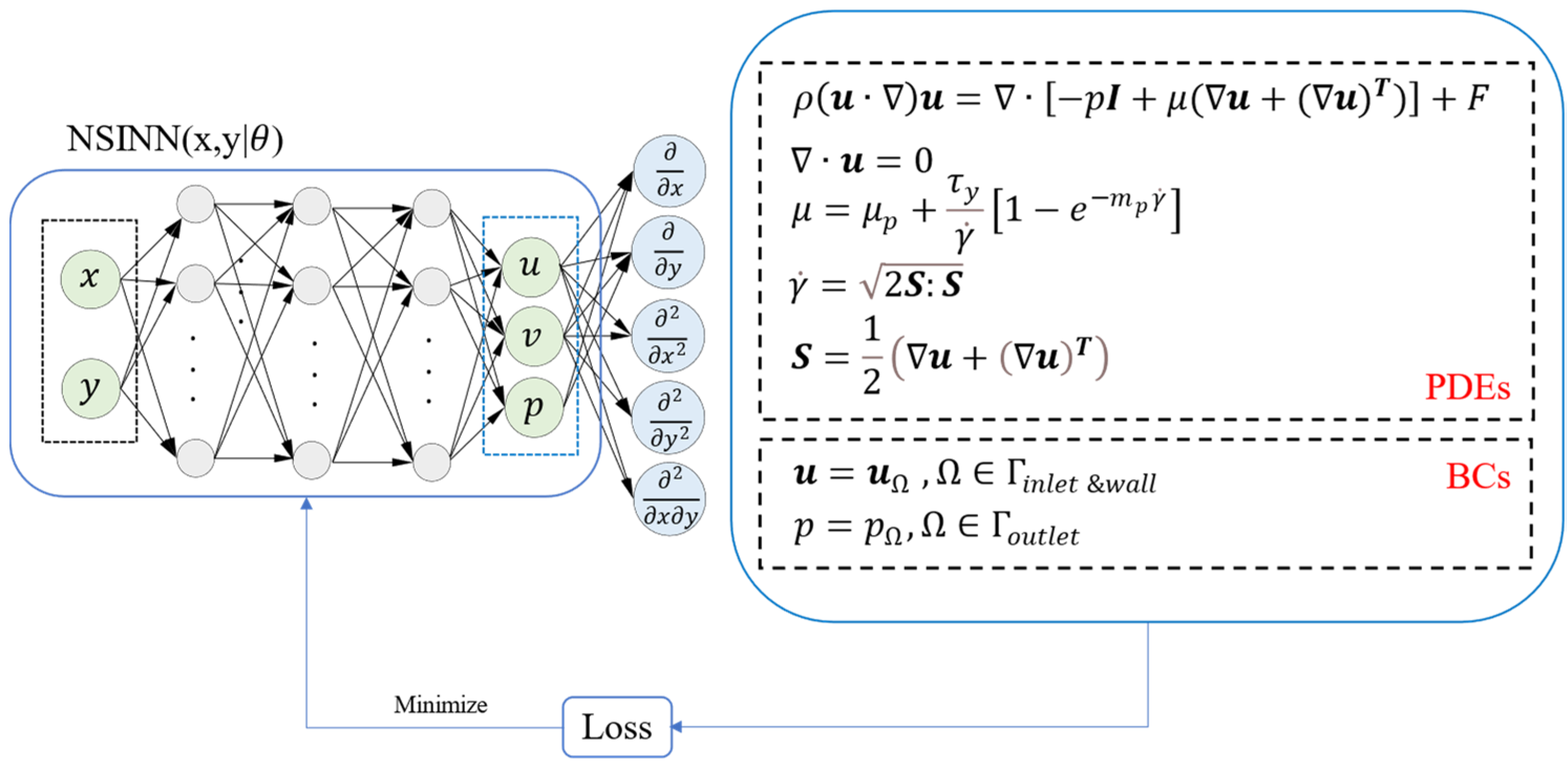
2.2. NSINN Architecture

We introduce a PINN-based model, named NSINN, which is designed to address incompressible laminar flow within the 3DCP process. This model approximates the solutions of the NS equations, utilizing spatial coordinates as inputs to predict the pressure and velocity fields. This approach leverages the strengths of neural networks while incorporating the underlying physical principles, offering a sophisticated tool for simulating fluid dynamics in 3DCP. Prior knowledge of the NS equations is introduced to the construction of the NSINN, which effectively regularizes the minimization procedure in the training of neural networks. A schematic illustration of the proposed NSINN architecture is shown in Figure 2.

As shown in Figure 2, $(x,y)$ is the location of the training points. $(u,v,p)$ is the velocity and pressure field. $u=u_{\Gamma }$ and $p=p_{\Gamma }$ are the boundary conditions applied in the geometry. The residuals from the NS equation (PDE) and boundary conditions (BC) are calculated and embedded into the loss function of the presented NSINN network. The NSINN is trained to find the best network parameter $\theta$ by minimizing the loss function. In the inlet, the velocity components u and v are specified (u = 2 cm/s and v = 0 cm/s). On the wall boundaries, no-slip conditions (u = 0 and v = 0) are implemented. At the outlet, pressure values are set to zero (p = 0).

The NSINN architecture consists of 6 hidden layers, while each layer contains 50 nodes in this study. $x$ and $y$ are the inputs and $u,v,p$ are the outputs of the NSINN. The structure of the NSINN can be expressed as Equation (9).

$$NSINN(x,y|\theta )=\sigma (\theta [\mathrm{x},\mathrm{y}])$$

(9)

where $\theta$ is the set of all weight matrices and bias vectors in the neural network. Here, $\theta =\{\mathit{W},\mathit{b}\}$; W is the weights; and b is the biases. The weights and biases are trained using a back-propagation algorithm. $\sigma (·)$ is the activation function used in the network. The hyperbolic tangent activation function is utilized as the activation function in the NSINN for its infinite differentiability [36].

$$Tanh\left(x\right)={\displaystyle \frac{e^x-e^{-x}}{e^x+e^{-x}}}$$

(10)

where the Tanh(x) is the hyperbolic tangent activation function. X is the input, and e stands for the exponential function. $\theta$ is trained by minimizing the loss function $\mathcal{L}\left(\theta \right|N_d)$, which consists of two parts: the Mean Square Error (MSE) from the data (${\mathcal{L}}_d\left(\theta \right|N_d)$) and the residuals from the equations and boundary conditions (${\mathcal{L}}_{pde}\left(\theta \right|N_d\left)\right)$, as shown in Equation (11). Even though PINNs are informed by physical laws, they still benefit from observational data to improve their accuracy and reliability. The MSE of the data is a measure of how well the network’s predictions match the actual observed data. This component is crucial for training the network to fit specific data points, ensuring that the model not only follows the physical equations but also aligns closely with empirical observations.

$$\mathcal{L}\left(\theta \right|N_d)={\mathcal{L}}_d(\theta \left|N_d\right)+{\mathcal{L}}_{pde}\left(\theta \right|N_d)$$

(11)

where $N_d$ is the training points randomly selected from the computing domain. ${\mathcal{L}}_d\left(\theta \right|N_d)$ is the MSE between the original data and the predictions, and ${\mathcal{L}}_{pde}\left(\theta \right|N_d)$ represents the residual from equations. Therefore, ${\mathcal{L}}_{pde}\left(\theta \right|N_d)$ consists of two parts and can be expressed using Equation (12).

$${\mathcal{L}}_{pde}\left(\theta \right|N_d)={\mathcal{L}}_{eq}(\theta \left|N_r\right)+{\mathcal{L}}_b\left(\theta \right|N_b)$$

(12)

where $N_r$ represents the training points in the region. $N_b$ is the number of points randomly selected from the boundary conditions. ${\mathcal{L}}_{eq}\left(\theta \right|N_r)$ is the residual from PDEs, while ${\mathcal{L}}_b\left(\theta \right|N_b)$ represents the residual from boundary conditions.

The calculation of ${\mathcal{L}}_{pde}\left(\theta \right|N_d)$ is based on the NS equations and the boundary conditions. Before incorporating the governing equations into the deep learning structure, the steady-state NS equations should be converted to their derivative forms so that the PDEs can be interpreted easily in the neural network. The 2D momentum equation in its derivative form is given by Equations (13) and (14) according to Equation (1).

$$\rho \left(u{\displaystyle \frac{du}{dx}}+v{\displaystyle \frac{du}{dy}}\right)=-{\displaystyle \frac{dp}{dx}}+\mu \left(2{\displaystyle \frac{d^{2}u}{d{x}^2}}+{\displaystyle \frac{d^{2}u}{d{y}^2}}+{\displaystyle \frac{d^{2}v}{dxdy}}\right)+F_x$$

(13)

$$\rho \left(u{\displaystyle \frac{dv}{dx}}+v{\displaystyle \frac{dv}{dy}}\right)=-{\displaystyle \frac{dp}{dy}}+\mu \left({\displaystyle \frac{d^{2}v}{d{x}^2}}+2{\displaystyle \frac{d^{2}v}{d{y}^2}}+{\displaystyle \frac{d^{2}u}{dydx}}\right)+F_y$$

(14)

The 2D mass equations in their derivative forms are given by Equation (15) according to Equation (2).

$${\displaystyle \frac{du}{dx}}+{\displaystyle \frac{dv}{dy}}=0$$

(15)

The residuals of the steady-state incompressible NS equations can be expressed using the following equations:

$$r_1={\displaystyle \frac{du}{dx}}+{\displaystyle \frac{dv}{dy}}$$

(16)

$$r_2=\rho \left(u{\displaystyle \frac{du}{dx}}+v{\displaystyle \frac{du}{dy}}\right)+{\displaystyle \frac{dp}{dx}}-\mu \left(2{\displaystyle \frac{d^{2}u}{d{x}^2}}+{\displaystyle \frac{d^{2}u}{d{y}^2}}+{\displaystyle \frac{d^{2}v}{dxdy}}\right)-F_x$$

(17)

$$r_3=\rho \left(u{\displaystyle \frac{dv}{dx}}+v{\displaystyle \frac{dv}{dy}}\right)+{\displaystyle \frac{dp}{dy}}-\mu \left({\displaystyle \frac{d^{2}v}{d{x}^2}}+2{\displaystyle \frac{d^{2}v}{d{y}^2}}+{\displaystyle \frac{d^{2}u}{dydx}}\right)-F_y$$

(18)

where $r_1$, $r_2$, and $r_3$ represent the residuals of each equation.

The calculation equations of ${\mathcal{L}}_d\left(\theta \right|N_d)$, ${\mathcal{L}}_{eq}\left(\theta \right|N_r)$, and ${\mathcal{L}}_b\left(\theta \right|N_b)$ are shown below.

$${\mathcal{L}}_d(\theta |N_d)={\displaystyle \frac{1}{N_d}}{\displaystyle {\sum }_{k=1}^{N_d}}\left\{{\left(u^k-{\widehat{u}}^k\right)}^2+{{(v}^k-{\widehat{v}}^k)}^2+(p^k-{\widehat{p}}^k)\right\}$$

(19)

$${\mathcal{L}}_{pde}(\theta |N_r)={\displaystyle \frac{1}{N_r}}{\displaystyle {\sum }_{k=1}^{N_r}}(r_1^2+r_2^2+r_3^2)$$

(20)

$${\mathcal{L}}_b(\theta |N_b)={\displaystyle \frac{1}{N_b}}{\displaystyle {\sum }_{k=1}^{N_b}}(r_{wall}^2+r_{inlet}^2+r_{outlet}^2)$$

(21)

where $r_{(·)}^2$ denotes the residual. $r_{wall}$, $r_{inlet}$, and $r_{outlet}$ stand for the residual calculated from the wall, inlet, and outlet boundaries, respectively.

Incorporating physical laws into the NSINN framework enhances its suitability in scenarios with limited data, which is a significant advantage considering the high cost and time-intensive nature of collecting experimental data for conventional deep learning-based neural network predictions. Furthermore, NSINN offers greater interpretability in understanding cement paste flow patterns compared to traditional data-driven approaches, such as standard neural networks. This interpretability is crucial for effectively learning and applying physical laws in the study of material properties.

A gradient-based optimizer, Adaptive Moment Estimation (Adam), is utilized to train the $\mathrm{N}\mathrm{S}\mathrm{I}\mathrm{N}\mathrm{N}(x,y|\theta )$. An initial learning rate of $1\times {10}^{-3}$ is specified. The learning rate is reduced by 1/10 every 20,000 iterations. A minimum learning rate of $1\times {10}^{-6}$ is defined, and the learning rate is not reduced further. After that, limited-memory Broyden–Fletcher–Goldfarb–Shanno (L-BFGS) [37] is used to minimize the loss function of $\mathrm{N}\mathrm{S}\mathrm{I}\mathrm{N}\mathrm{N}(x,y|\theta )$ to obtain the best parameter ${\theta }^{*}$ because of the good convergence speed of L-BFGS. The total training number for the $\mathrm{N}\mathrm{S}\mathrm{I}\mathrm{N}\mathrm{N}(x,y|\theta )$ is 9000, including 8000 points in the domain and 1000 points in the boundary.

In our study, we implemented the $\mathrm{N}\mathrm{S}\mathrm{I}\mathrm{N}\mathrm{N}(x,y|\theta )$ alongside a traditional ANN for comparative analysis to simulate the NS equations relevant to the 3D printing process. The ANN was structured identically to the NSINN, featuring one input layer, one output layer, and six hidden layers. Both models’ training processes were governed by a loss function that calculates the MSE of the training data, and they shared the same training strategy. The NSINN and ANN models were developed using the PyTorch framework. In addition, we conducted a direct numerical simulation using CFD modeling to provide a benchmark solution. The performance evaluation of the NSINN and ANN, in terms of accuracy and robustness, was conducted by comparing their results to the exact solution derived from the CFD simulation. All simulations were carried out on a computing platform equipped with a 2.3 GHz Quad-Core Intel Core i7 CPU, 16 GB 3733 MHz LPDDR4X memory, and an Intel Iris Plus Graphics 1536 MB GPU. However, it is noteworthy that GPUs were not utilized in these simulations. Given the relatively small size of the dataset used in these methods, CPUs were found to offer performance comparable to that of GPUs.

3. Results

First, the steady-state NS Equations proposed in Section 2.1 are simulated by three different approaches, namely, the NSINN, the ANN, and CFD. Then, three different geometries with different R values are simulated to interpret the impact of nozzle diameter on the distribution of shear stress as well as the extrudability.

3.1. NS Equation Evaluation

As a mesh-free simulation approach, the NSINN is trained using randomly selected locations $(x,y)$. Figure 3a illustrates this setup, where the domain contains $N_r=8000$ training points and the boundary is defined by $N_b=1000$ points. In both the NSINN and ANN models, the training points, represented as black dots in the figure, follow a pseudo-random distribution.

The training processes for the NSINN and ANN adhere to the same strategy. The correlation between training loss and the number of epochs for these two networks is depicted in Figure 3b. This visual representation aids in understanding how the models learn and evolve over time, providing insights into their training dynamics and efficiency.

In Figure 3b, each point represents the mean value of the loss in 1000 epochs. The light green area and purple area stand for the standard deviation of the loss of the ANN and NSINN, respectively. At first, the loss of the NSINN is higher than that of the ANN. This is because the loss of the NSINN contains higher residuals from the physical equations and boundary conditions compared to the ANN, but it is noteworthy that the loss of the NSINN drops faster than that of the ANN, especially from 0 to 20,000 epochs. It can be interpreted that the embedded PDEs help the network constrain the training procedure, which makes the loss drop dramatically. It is interesting that the loss of the ANN started to fluctuate during the 60,000 to 100,000 epochs, which means the ANN cannot update its weights and biases effectively during the training. However, for the NSINN, the loss continues to decrease until 100,000 epochs.

The trained NSINN and ANN are then utilized to predict the geometry, as shown in Figure 1. Also, the CFD is used to simulate the flow condition of the cementitious materials in the domain. The predicted velocity and pressure fields by the NSINN and traditional ANN as well as the CFD reference are shown in Figure 4.

The first row represents the results from CFD simulations, and it is used as the reference to calculate the prediction errors in the NSINN and ANN. The second row is the prediction results from a traditional ANN, while the third row represents the prediction results from the NSINN. As we can see, the simulation results from the NSINN are almost the same as those of the CFD reference, while the prediction results from traditional ANN are not consistent with those of the CFD reference. This issue primarily arises from the ANN’s over-reliance on training points. Given the highly nonlinear nature of the NS equations, predicting these equations accurately using only the MSE in the data as the loss function proves to be extremely challenging. This complexity underscores the need for more sophisticated approaches or loss functions that can better capture and adapt to the intricate dynamics of the NS equations.

To assess the average performance and robustness of each method, all models were executed three times. The mean and standard deviation of the MSE were calculated from these runs. Figure 5 presents box plots illustrating the distribution of the MSE in predicting the flow behaviors of cementitious materials.

The average MSE values obtained from the NSINN for the u, v, and p components are $1.25\times {10}^{-4}$, $1.85\times {10}^{-5}$, and $3.91\times {10}^{-3}$, respectively. In comparison, the ANN yielded average MSEs of $5.88\times {10}^{-2}$, $4.17\times {10}^{-3}$, and $1.72\times {10}^{-2}$, respectively, for the same components. These results indicate that the NSINN outperforms the ANN in terms of flow pattern prediction accuracy.

Furthermore, the NSINN demonstrates greater robustness, evidenced by its smaller standard deviation in predictions compared to the ANN. Specifically, the standard deviations for the NSINN in predicting u, v, and p are $1.43\times {10}^{-3}$, $2.52\times {10}^{-5}$, and $3.38\times {10}^{-4}$, respectively. In contrast, the ANN shows standard deviations of $1.55\times {10}^{-2}$, $9.11\times {10}^{-5}$, and $1.58\times {10}^{-2}$, respectively, for the same components. This indicates that the NSINN not only provides more accurate predictions but also maintains more consistent performance across different runs than the ANN.

The velocity distribution on the outlet is important for the application of 3DCP as it has an impact on extrudability and printability performance. This is because the velocity distribution of cementitious materials in the printing barrel can change the shear rate distribution, which can lead to a change in viscosity as the cement paste is a thixotropic fluid. Therefore, the velocity and pressure distribution in the barrel (x = 18 cm) and on the outlet (x = 21 cm) are monitored and studied. The comparison between the CFD reference, NSINN, and ANN when x = 18 cm and x = 21 cm (outlet) is shown in Figure 6.

As we can see from Figure 6, the red line represents the result from the CFD reference. The blue dashed line stands for the results from the NSINN, while the black dash-dot line stands for the prediction from the ANN. The proposed NSINN aligns better with the reference than the traditional ANN on the velocity and pressure field. It is noteworthy that the ANN performed in the outlet boundary compared to the prediction inside the domain. It is mainly because the performance of the ANN is totally dependent on the training points, but there are fewer training points in the boundary than inside the geometry. At the outlet, the performance of the NSINN is influenced by the imposed boundary conditions, which help ensure accurate predictions in this region. It is interesting to see that the pressure value on the outlet predicted by the ANN is much higher than that of the reference. It is mainly because the ANN learns from the nearby points (close to the outlet), whose pressure is higher than 0.

The computational cost is a critical factor in practical simulations, particularly for models with a large number of parameters or complex geometries. An efficient simulation tool not only conserves computational resources but also speeds up the simulation process. One practical way to gauge the computational cost of different methods is by comparing the time required for the prediction. Figure 7 illustrates this comparison, showing the prediction times for the NSINN, the ANN, and CFD, thereby providing insights into the efficiency of each method in terms of computational resource utilization.

Figure 7 reveals that the average prediction times for the NSINN, the ANN, and CFD are 0.039 s, 0.014 s, and 3.37 s, respectively. This indicates that the time required for CFD simulations is at least 100 times longer than that for the neural network-based methods, including both the ANN and NSINN. Such a comparison highlights that while CFD offers high accuracy, it is also a computationally intensive approach.

In contrast, mesh-free numerical methods like the NSINN demonstrate significantly faster simulation speeds compared to traditional mechanism-based methods like CFD. The advantage of mesh-free methods is particularly evident in their setup and implementation processes. Without the necessity for mesh generation, the NSINN can be implemented more simply and directly, which is especially beneficial for problems involving irregular boundaries or higher-dimensional spaces.

In mesh-based methods, a considerable portion of the preprocessing time is dedicated to generating and refining the mesh. This process becomes increasingly complex and time-consuming when dealing with intricate geometries. Therefore, the efficiency of mesh-free methods like the NSINN in terms of computational time is a substantial advantage in practical simulations.

It is interesting to find that the prediction time of the NSINN is a little longer than that of the ANN. It is mainly because the NSINN needs to calculate the residual from the embedded PDEs, which would consume more computational power and, therefore, use a longer time. It is noteworthy that the NSINN can work as a surrogate method, which is much faster and computationally efficient compared to the traditional CFD method as it uses much less time and provides promising accuracy.

3.2. Evaluation of the Extrudability Using NSINN

Since the NSINN has a high performance in accuracy and efficiency in PDE simulations, it is used as an example to study the influence of the nozzle diameter on extrudability in 3DCP. It is noteworthy that extrudability refers to the ability of the cementitious material to be forced or extruded through the nozzle to create a continuous stream with a specific cross-sectional profile. There is no universal equation to describe extrudability, but it is related to the consistency and rheology of the materials. Therefore, the velocity and shear stress distribution are studied, which is related to the cementitious material’s consistency and rheology. As defined in Equation (6), the ratio R is used as our evaluation parameter. In the following section, the impact of R on the velocity field and shear rate is studied, as shown in Figure 8.

As shown in Figure 8a, it is interesting that with a smaller R, the peak velocity in the barrel increases. The value of R has an impact on the velocity both in the pipeline and the nozzle. Figure 8b,c shows the velocity field when x = 18 cm and x = 22 cm, respectively. It is apparent that an R value of 0.25 has a larger peak velocity than the other values. In other words, the cementitious material is supposed to be forced at a higher speed in the same printing process when the diameter of the nozzle is smaller. It means that there is a higher requirement for the rheology and particle size of the material when using a smaller nozzle.

The shear rate experienced by the material can be influenced by the velocity distribution according to Equations (6) and (7). Thus, the shear rate is also predicted by the NSINN in three different Rs, which are 0.25, 0.5, and 0.75. The predicted result is shown in Figure 9a.

As we can see from Figure 9a, the distribution of the shear rate is non-uniform. The shear rate of cementitious materials around the nozzle is larger than in the pipeline. Moreover, the shear rate of the cement near the wall is larger than in the middle. That is because the cementitious material will adhere to the surface and there will be no relative motion between the boundary and the fluid immediately in contact with it. A high shear rate distribution in the 3D printing barrel would cause a lower viscosity and lower yield stress in the cementitious materials. This is because the cementitious material is a shear thinning material. At low shear rates, the cement paste typically has a higher viscosity and thus higher resistance to flow, resulting in a relatively steep slope in the shear stress vs. shear rate plot. As the shear rate increases, the material undergoes shear thinning and its viscosity decreases. For the printability of 3DCP, we anticipate that the material will have a high viscosity and yield stress, and it can help the printed material hold the weight from the upper layers.

The relationship between R and the shear rate is also studied, as shown in Figure 9b. This simulation connects the macroscopic design element, specifically the printing barrel’s diameter, with the microscopic aspect of the shear rate, thereby establishing a multiscale relationship. This relationship is captured through physics-based modeling and simulation, highlighting the intricate interplay between different scales in the printing process. It is interesting to see that the average shear rate decreases with an increase in R. It means that when the input velocity is constant, a larger nozzle diameter can help decrease the shear rate and then increase the viscosity of the printed cement paste. In other words, a larger nozzle size can help the material gain a higher printability.

4. Conclusions

In this work, we proposed a NSINN as a surrogate approach to predict the localized flow behavior of the cementitious materials during the 3D printing process. Below are the key findings from this study:

• We identify the weakness of the traditional neural networks and improve it with physics-driven rules by embedding the NS equations into the loss function of the network. It is successfully utilized to deliver accurate, stable, and computationally efficient simulation strategies for cementitious materials in 3DCP tasks.
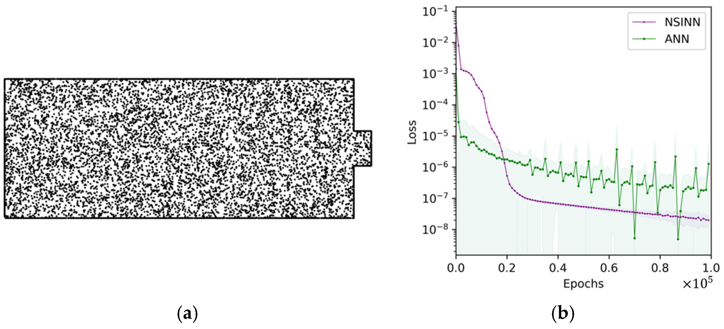
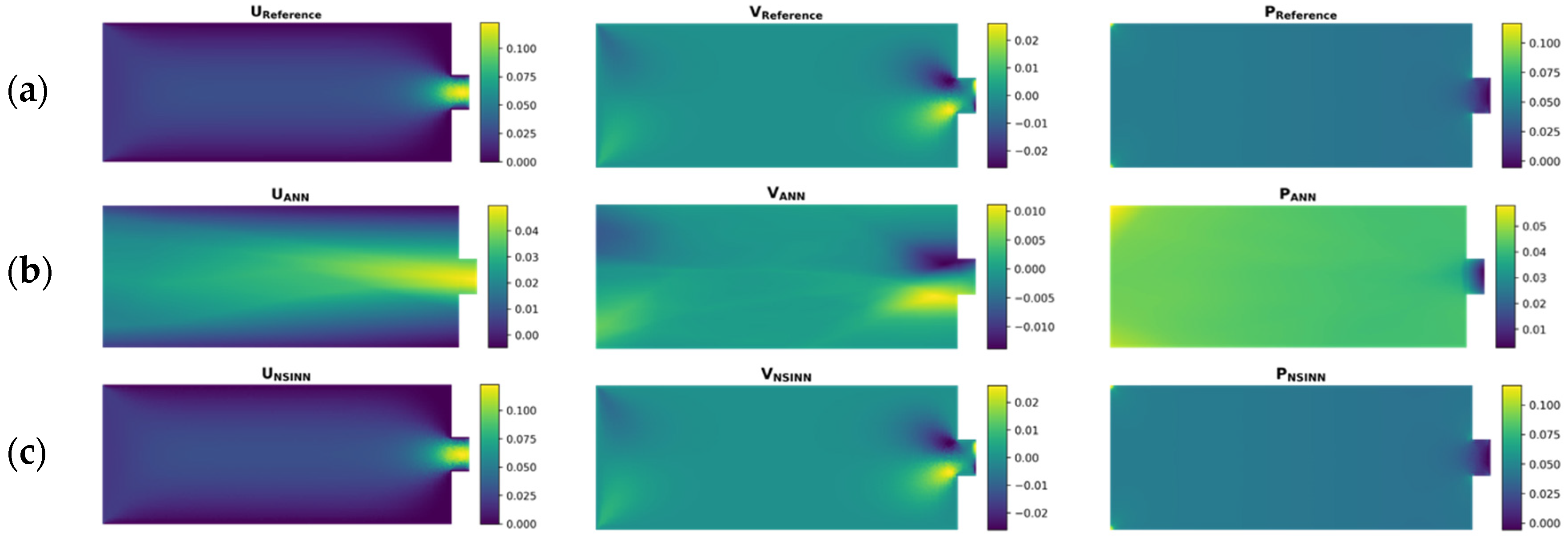
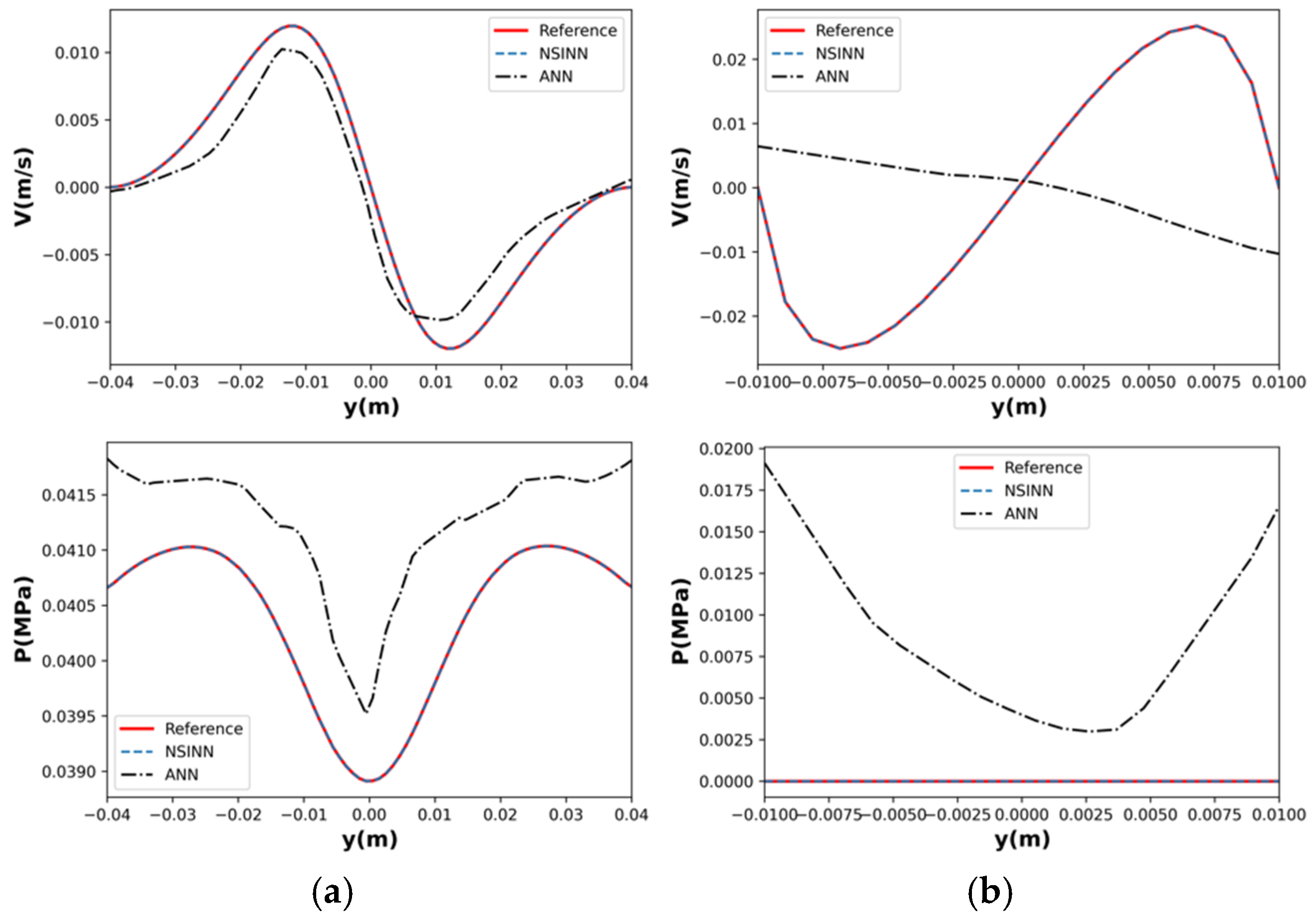
• The proposed NSINN is compared to the ANN and CFD in terms of accuracy and efficiency. The ANN is designed to have the same architecture as the NSINN but without adding any physical rules. The CFD simulation result is used as a reference to evaluate the performance of the NSINN and ANN.
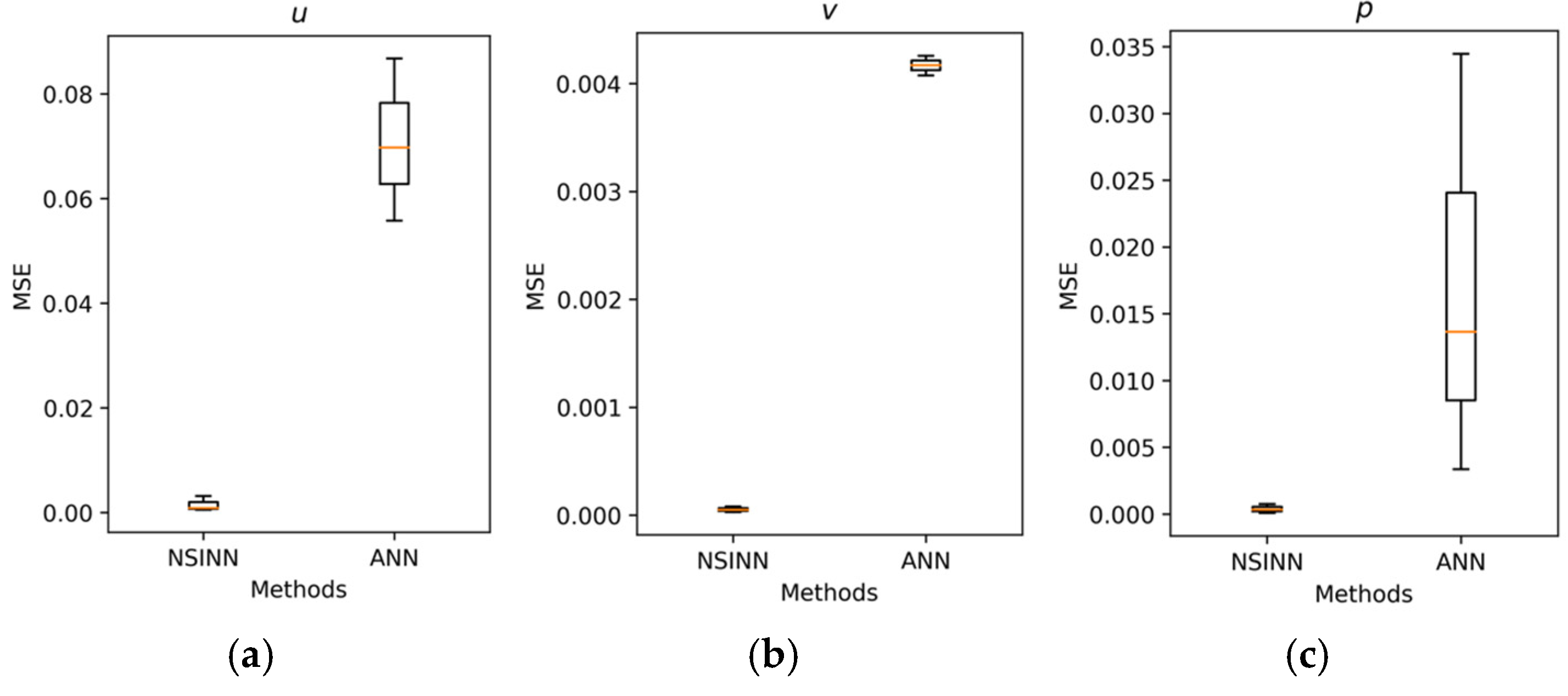
• The prediction results show that the presented NSINN promises higher accuracy in simulating the 3DCP process than the ANN. Moreover, it has a lower standard deviation than the ANN, which means it is more stable and robust in predicting the flow patterns of cementitious materials in the printing barrel.
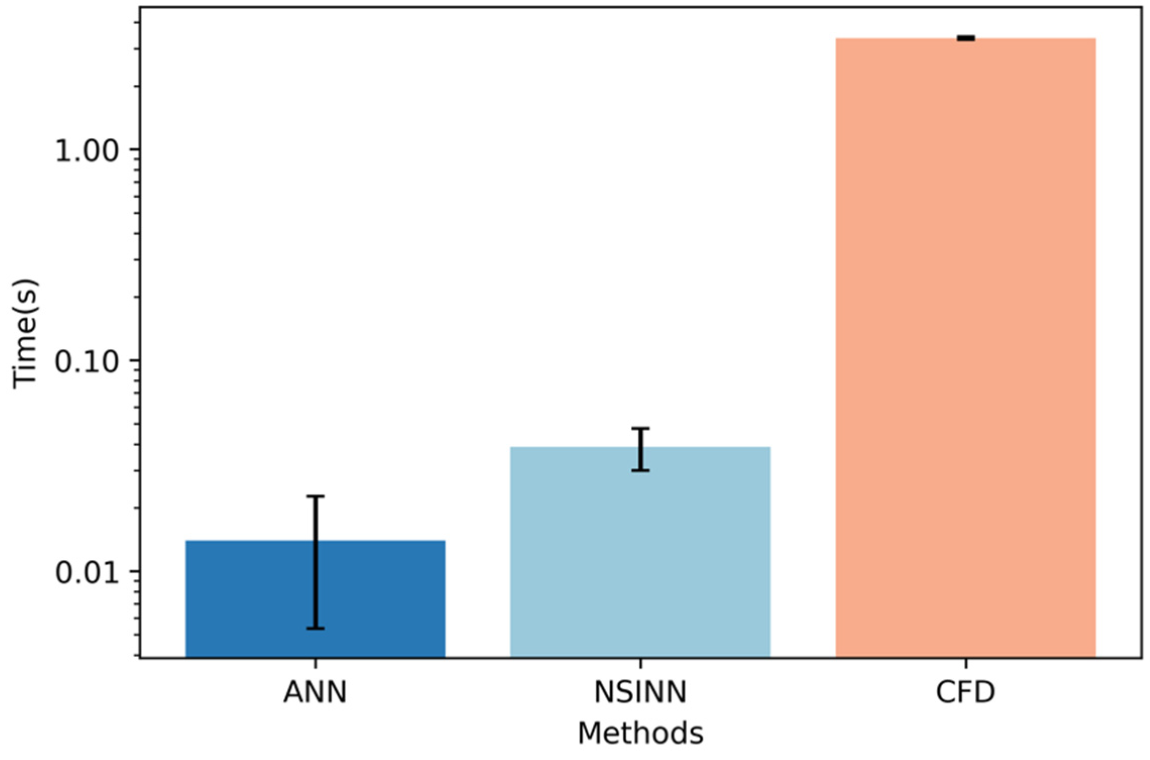
• It is noteworthy that the inference time for the NSINN to predict a model is 0.039 s, which is almost 100 times lower than the traditional mesh-based method, namely, CFD (3.37 s). In other words, the NSINN promises an excellent trade-off between accuracy and efficiency in simulations.
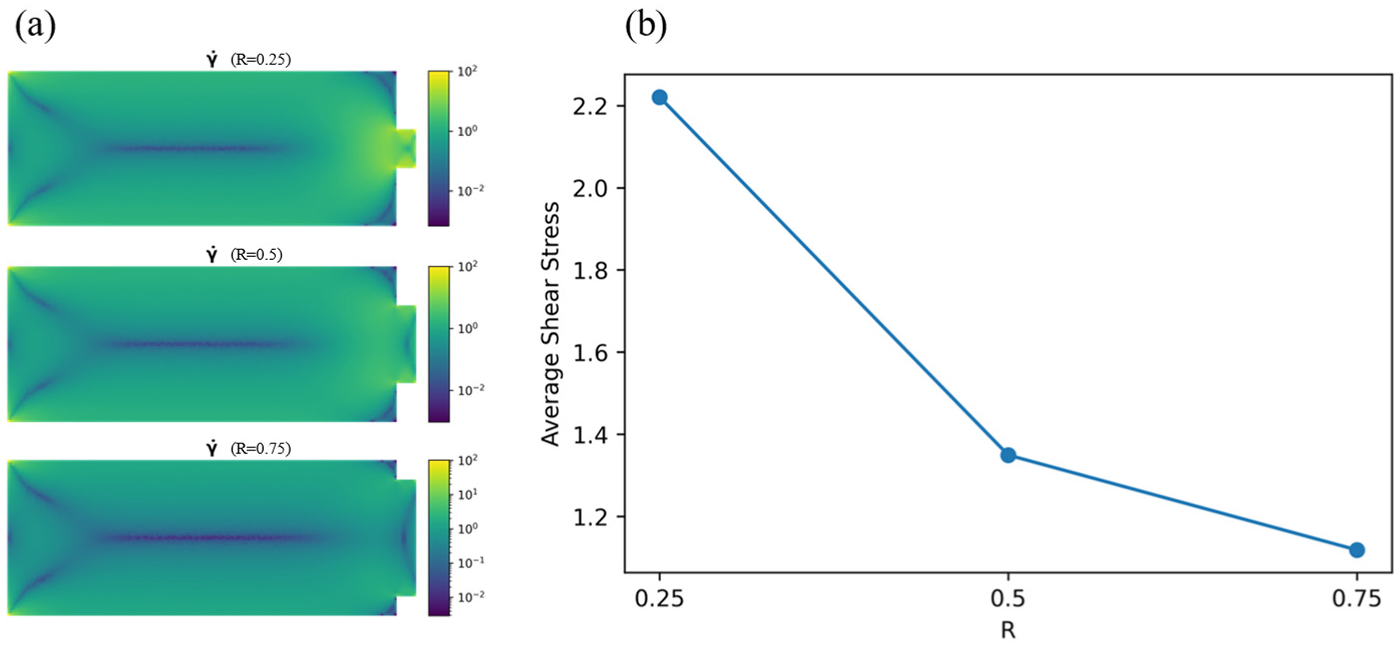
• Due to the high accuracy of the NSINN, it is used to study the influence of R (the ratio between the diameter of the pipeline and that of the nozzle) on extrudability in 3DCP. It shows that the size of the nozzle would have an impact on the velocity distribution of cementitious materials. Moreover, the distribution of shear rates experienced by the material is not uniformly distributed. The ratio of R is studied and analyzed to figure out its relationship with the extrudability and printability of the 3D printing process. It shows that with a higher R, the experienced shear rate of the cementitious material would increase, thus leading to a lower viscosity and yield stress. Also, the average shear stress has a negative relationship with R.

We anticipate that this study will contribute to the growing body of knowledge about the application of PINNs for 3DCP simulations. The findings of this study have the potential to enhance our understanding of cement material flow patterns in 3D printing barrels and offer insights into the performance of PINNs compared to traditional simulation methods. Furthermore, this research could pave the way for more efficient and accurate simulations in the field of fluid dynamics, enabling improved design and optimization of 3DCP processes. This study can also be used in other material-printing processes like recycled aggregate-based cement, cementitious mixtures, and ceramic as all of these materials follow the NS equations, and during the 3D printing work, the only difference among them is the viscosity and the geometry. In the future, we plan to expand the application of the NSINN by testing it on more complex geometries and under varying boundary conditions. Also, a sensitivity analysis of the NSINN on model parameters like hidden layers, activation functions, and the choice of learning rate will be conducted. Future work will also explore the direct impact of flow dynamics on surface quality.

References

1. Long, W.-J.; Tao, J.-L.; Lin, C.; Gu, Y.-C.; Mei, L.; Duan, H.-B.; Xing, F. Rheology and buildability of sustainable cement-based composites containing micro-crystalline cellulose for 3D-printing. J. Clean. Prod. 2019, 239, 118054. [Google Scholar] [CrossRef]
2. Marchment, T.; Sanjayan, J. Mesh reinforcing method for 3D Concrete Printing. Autom. Constr. 2020, 109, 102992. [Google Scholar] [CrossRef]
3. Rehman, A.U.; Kim, J.-H. 3D concrete printing: A systematic review of rheology, mix designs, mechanical, microstructural, and durability characteristics. Materials 2021, 14, 3800. [Google Scholar] [CrossRef]
4. Bhattacherjee, S.; Basavaraj, A.S.; Rahul, A.; Santhanam, M.; Gettu, R.; Panda, B.; Schlangen, E.; Chen, Y.; Copuroglu, O.; Ma, G. Sustainable materials for 3D concrete printing. Cem. Concr. Compos. 2021, 122, 104156. [Google Scholar] [CrossRef]
5. Bong, S.H.; Xia, M.; Nematollahi, B.; Shi, C. Ambient temperature cured ‘just-add-water’geopolymer for 3D concrete printing applications. Cem. Concr. Compos. 2021, 121, 104060. [Google Scholar] [CrossRef]
6. Feng, P.; Meng, X.; Chen, J.-F.; Ye, L. Mechanical properties of structures 3D printed with cementitious powders. Constr. Build. Mater. 2015, 93, 486–497. [Google Scholar] [CrossRef]
7. Lee, H.; Kim, J.-H.J.; Moon, J.-H.; Kim, W.-W.; Seo, E.-A. Correlation between pore characteristics and tensile bond strength of additive manufactured mortar using X-ray computed tomography. Constr. Build. Mater. 2019, 226, 712–720. [Google Scholar] [CrossRef]
8. Chen, X.; Lam, Y.; Tan, K.; Chai, J.; Yu, S. Shear-induced particle migration modelling in a concentrated suspension flow. Model. Simul. Mater. Sci. Eng. 2003, 11, 503. [Google Scholar] [CrossRef]
9. Arunothayan, A.R.; Nematollahi, B.; Khayat, K.H.; Ramesh, A.; Sanjayan, J.G. Rheological characterization of ultra-high performance concrete for 3D printing. Cem. Concr. Compos. 2023, 136, 104854. [Google Scholar] [CrossRef]
10. Feys, D. How much is bulk concrete sheared during pumping? Constr. Build. Mater. 2019, 223, 341–351. [Google Scholar] [CrossRef]
11. Vallurupalli, K.; Farzadnia, N.; Khayat, K.H. Effect of flow behavior and process-induced variations on shape stability of 3D printed elements–A review. Cem. Concr. Compos. 2021, 118, 103952. [Google Scholar] [CrossRef]
12. Choi, M.; Roussel, N.; Kim, Y.; Kim, J. Lubrication layer properties during concrete pumping. Cem. Concr. Res. 2013, 45, 69–78. [Google Scholar] [CrossRef]
13. Le, T.T.; Austin, S.A.; Lim, S.; Buswell, R.A.; Law, R.; Gibb, A.G.; Thorpe, T. Hardened properties of high-performance printing concrete. Cem. Concr. Res. 2012, 42, 558–566. [Google Scholar] [CrossRef]
14. Zhang, Y.; Zhang, Y.; Liu, G.; Yang, Y.; Wu, M.; Pang, B. Fresh properties of a novel 3D printing concrete ink. Constr. Build. Mater. 2018, 174, 263–271. [Google Scholar] [CrossRef]
15. Raissi, M.; Yazdani, A.; Karniadakis, G.E. Hidden fluid mechanics: Learning velocity and pressure fields from flow visualizations. Science 2020, 367, 1026–1030. [Google Scholar] [CrossRef] [PubMed]
16. Chorin, A.J. Numerical solution of the Navier-Stokes equations. Math. Comput. 1968, 22, 745–762. [Google Scholar] [CrossRef]
17. Rizzieri, G.; Ferrara, L.; Cremonesi, M. Numerical simulation of the extrusion and layer deposition processes in 3D concrete printing with the Particle Finite Element Method. Comput. Mech. 2023, 73, 277–295. [Google Scholar] [CrossRef]
18. Reinold, J.; Nerella, V.N.; Mechtcherine, V.; Meschke, G. Extrusion process simulation and layer shape prediction during 3D-concrete-printing using the Particle Finite Element Method. Autom. Constr. 2022, 136, 104173. [Google Scholar] [CrossRef]
19. Jayathilakage, R.; Rajeev, P.; Sanjayan, J. Extrusion rheometer for 3D concrete printing. Cem. Concr. Compos. 2021, 121, 104075. [Google Scholar] [CrossRef]
20. Comminal, R.; da Silva, W.R.L.; Andersen, T.J.; Stang, H.; Spangenberg, J. Modelling of 3D concrete printing based on computational fluid dynamics. Cem. Concr. Res. 2020, 138, 106256. [Google Scholar] [CrossRef]
21. Mollah, M.T.; Comminal, R.; da Silva, W.R.L.; Šeta, B.; Spangenberg, J. Computational fluid dynamics modelling and experimental analysis of reinforcement bar integration in 3D concrete printing. Cem. Concr. Res. 2023, 173, 107263. [Google Scholar] [CrossRef]
22. Amalinadhi, C.; Palar, P.S.; Stevenson, R.; Zuhal, L. On Physics-Informed Deep Learning for Solving Navier-Stokes Equations. In Proceedings of the AIAA SCITECH 2022 Forum, San Diego, CA, USA, 3–7 January 2022; p. 1436. [Google Scholar]
23. Zhang, T.; Wang, D.; Lu, Y. ECSNet: An Accelerated Real-Time Image Segmentation CNN Architecture for Pavement Crack Detection. IEEE Trans. Intell. Transp. Syst. 2023, 24, 15105–15112. [Google Scholar] [CrossRef]
24. Zhang, T.; Wang, D.; Mullins, A.; Lu, Y. Integrated APC-GAN and AttuNet Framework for Automated Pavement Crack Pixel-Level Segmentation: A New Solution to Small Training Datasets. IEEE Trans. Intell. Transp. Syst. 2023, 24, 4474–4481. [Google Scholar] [CrossRef]
25. Zhang, T.; Wang, D.; Lu, Y. A data-centric strategy to improve performance of automatic pavement defects detection. Autom. Constr. 2024, 160, 105334. [Google Scholar] [CrossRef]
26. Zhang, T.; Wang, D.; Lu, Y. Machine learning-enabled regional multi-hazards risk assessment considering social vulnerability. Sci. Rep. 2023, 13, 13405. [Google Scholar] [CrossRef]
27. Zhang, T.; Smith, A.; Zhai, H.; Lu, Y. LSTM+ MA: A Time-Series Model for Predicting Pavement IRI. Infrastructures 2025, 10, 10. [Google Scholar] [CrossRef]
28. Zhang, T.; Wang, D.; Lu, Y. Benchmark Study on a Novel Online Dataset for Standard Evaluation of Deep Learning-based Pavement Cracks Classification Models. KSCE J. Civ. Eng. 2024, 28, 1267–1279. [Google Scholar] [CrossRef]
29. Rahman, M.A.; Zhang, T.; Lu, Y. PINN-CHK: Physics-informed neural network for high-fidelity prediction of early-age cement hydration kinetics. Neural Comput. Appl. 2024, 36, 13665–13687. [Google Scholar] [CrossRef]
30. Karniadakis, G.E.; Kevrekidis, I.G.; Lu, L.; Perdikaris, P.; Wang, S.; Yang, L. Physics-informed machine learning. Nat. Rev. Phys. 2021, 3, 422–440. [Google Scholar] [CrossRef]
31. Lu, L.; Meng, X.; Mao, Z.; Karniadakis, G.E. DeepXDE: A deep learning library for solving differential equations. SIAM Rev. 2021, 63, 208–228. [Google Scholar] [CrossRef]
32. Cheng, C.; Zhang, G.-T. Deep learning method based on physics informed neural network with resnet block for solving fluid flow problems. Water 2021, 13, 423. [Google Scholar] [CrossRef]
33. Cai, S.; Wang, Z.; Wang, S.; Perdikaris, P.; Karniadakis, G.E. Physics-informed neural networks for heat transfer problems. J. Heat Transf. 2021, 143, 060801. [Google Scholar] [CrossRef]
34. Bai, X.-D.; Zhang, W. Machine learning for vortex induced vibration in turbulent flow. Comput. Fluids 2022, 235, 105266. [Google Scholar] [CrossRef]
35. Chiu, P.-H.; Wong, J.C.; Ooi, C.; Dao, M.H.; Ong, Y.-S. CAN-PINN: A fast physics-informed neural network based on coupled-automatic–numerical differentiation method. Comput. Methods Appl. Mech. Eng. 2022, 395, 114909. [Google Scholar] [CrossRef]
36. Zhang, T.; Wang, D.; Lu, Y. RheologyNet: A physics-informed neural network solution to evaluate the thixotropic properties of cementitious materials. Cem. Concr. Res. 2023, 168, 107157. [Google Scholar] [CrossRef]
37. Nocedal, J. Updating quasi-Newton matrices with limited storage. Math. Comput. 1980, 35, 773–782. [Google Scholar] [CrossRef]
Figure 1. Diagram of the computation model.
Buildings 15 00275 g001
Figure 2. Overview of the NSINN framework.
Buildings 15 00275 g002
Figure 3. (a) Distribution of the training points used in NSINN and ANN. (b) Relationship between loss and epochs during the training procedure of the NSINN and ANN.
Buildings 15 00275 g003
Figure 4. Predicted velocity and pressure fields from different methods: (a) reference; (b) ANN; and (c) NSINN.
Buildings 15 00275 g004
Figure 5. Boxplots of the MSE for the NSINN and ANN in predicting different flow parameters of cementitious materials: (a) u; (b) v; and (c) p.
Buildings 15 00275 g005
Figure 6. Distribution of velocity and pressure fields when (a) x = 18 cm and (b) x = 21 cm (outlet).
Buildings 15 00275 g006aBuildings 15 00275 g006b
Figure 7. Time used in the simulation for the ANN, NSINN, and CFD.
Buildings 15 00275 g007
Figure 8. Impact of R on the velocity field and shear rate. (a) The distribution of the velocity field with different R values (0.25, 0.5, or 0.75); (b) the velocity field when x = 18 cm; and (c) the velocity field when x = 22 cm.
Buildings 15 00275 g008
Figure 9. (a) Distribution of the shear rate with different R values (0.25, 0.5, or 0.75). (b) The relationship between R and average shear stress.
Buildings 15 00275 g009